HIGH SPEED ROTARY PULSE WIDTH MODULATED ON/OFF VALVE

Proceedings of ASME-IMECE’07 2007 ASME International Mechanical Engineering Congress and RD&D Expo November 11-15, 2007, Seattle, Washington USA

IMECE2007-42559 HIGH SPEED ROTARY PULSE WIDTH MODULATED ON/OFF VALVE ∗

Haink C. Tu, Michael B. Rannow, James D. Van de Ven, Meng Wang, Perry Y. Li†and Thomas R. Chase Center for Compact and Efficient Fluid Power Department of Mechanical Engineering University of Minnesota 111 Church St. SE Minneapolis, MN 55455 Email: {tuxxx021,rann0018,vandeven,wang134,pli,trchase}@me.umn.edu

ABSTRACT

1 Introduction On/off (or digital) valve based control of hydraulic systems is an energy efficient alternative to control via throttling valves. In either the on or the off state, energy loss is minimized since either the pressure drop across the valve is small or the flow through it is zero. When the on/off valve is pulse width modulated, the average pressure or flow can be controlled. Our previous papers [7] and [6] have proposed and modeled the use of a PWM on/off valve with a fixed displacement pump to achieve the functionality of a variable displacement pump. A critical requirement for practical on/off valve based control is the availability of high speed on/off valves. High speed valves improve system efficiency, increase control bandwidth, and reduce output pressure ripple. Commercial on/off valves typically have transition times on the order of 20ms for flow rates of 5l/m-40l/m. Digital valve control with current valves demonstrate a noticeable decrease in system efficiency when operating at PWM frequencies greater than 10Hz [6]. A limitation in conventional valve designs based on linear spool or poppet movement is that the spool/poppet must be started and stopped during each on/off cycle. The power required to actuate the valve is proportional to the 3rd power of the PWM frequency. In this paper, we present a novel fluid driven unidirectional rotary PWM on/off valve design. Our valve spool achieves rotary motion by capturing momentum from the fluid that it meters. Since the spool rotates at a near constant velocity, the power required drive the valve only needs to overcome viscous friction, which is proportional to the frequency squared.

A key enabling technology to effective on/off valve based control of hydraulic systems is the high speed on/off valve. High speed valves improve system efficiency, offer faster control bandwidth, and produce smaller output pressure ripples. Current valves rely on the linear translation of a spool or poppet to meter flow. The valve spool must reverse direction twice per PWM cycle. This constant acceleration and deceleration of the spool requires a power input proportional to the PWM frequency cubed. As a result, current linear valves are severely limited in their switching frequencies. In this paper, we present a novel PWM on/off valve design that is based on a unidirectional rotary spool. The on/off functionality of our design is achieved via helical barriers that protrude from the surface of a cylindrical spool. As the spool rotates, the helical barriers selectively channel the flow to the application (on) or to tank (off). The duty ratio is controlled by altering the axial position of the spool. Since the spool no longer accelerates or decelerates during operation, the power input to drive the valve must only compensate for viscous friction, which is proportional to the PWM frequency squared. We predict that our current design, sized for a nominal flow rate of 40l/m, can achieve a PWM frequency of 84Hz. This is roughly a 400% improvement over current designs. This paper presents our valve concept, design equations, and an analysis of predicted performance. A simulation of our design is also presented.

A number of high speed hydraulic solenoid or piezo-electric 1

c 2007 by ASME Copyright

Figure 2.

Figure 1.

Diagram of internal geometry

path between application and tank. The duty ratio, or proportion per PWM cycle that the flow is directed to the application, is controlled by changing the axial position of the spool. By translating the spool upward relative to the inlet, the inlet will remain connected to the tank region for a greater portion per rotation of the spool. This decreases the duty ratio. The opposite effect will occur if the spool is translated downwards relative to the inlet. The rotary motion of our valve spool is achieved by extracting momentum from the fluid itself as the valve apportions flow to the application and to tank. The sleeve contains an internal pressure rail (see Fig. 4) that feeds tangential inlet nozzles, which create the fluid momentum. As the high speed fluid is transferred from the inlet nozzles to the valve spool, the helical barriers act as turbine blades to capture momentum from the fluid and direct it inward toward the center of the spool. As the fluid is directed inward, the momentum in the fluid is transferred to angular momentum in the spool. Once the fluid is at the center of the spool, it is forced to flow axially through an internal axial passageway that leads to the outlet stage turbine (see Fig. 2). The outlet stage turbine, similar in functionality to a lawn sprinkler, re-accelerates the flow outward and tangential to the spool. The outlet stage reverses the direction of the fluid relative to the inlet stage, which results in a reaction torque on the spool. By utilizing the fluid that must already pass through the valve for actuation, our selfspinning concept does not require an additional power source for operation. The self-spinning design is further enhanced by the 3-way configuration of our valve. The 3-way design continuously feeds fluid through the valve spool regardless of whether the flow is directed to application or tank. This allows the spool to rotate regardless of duty ratio. When combined with a 4-way directional valve, the 3-way functionality of our spool allows the system to operate as both a pump and as a motor. Our valve is packaged as an integrated pump cover/sleeve that can be bolted directly onto existing fixed displacement pumps. This integrated packaging allows us to minimize the inlet volume between the pump and valve (see Fig. 8), thus reducing

Diagram of 3-way rotary spool

actuated linear on/off valves have been proposed since the early 1990’s. Yokota et al. [8] and Lu et al. [10] achieved quick end-toend spool/poppet movement using piezo-electric materials, while Kajima et al. [9] investigated the development of a high speed linear solenoid valve for control in diesel engines. A unidirectional rotary spool valve was proposed by Cyphelly et al. [11] in 1980 for use with hydraulic applications, while Royston et al. [12] proposed a unidirectional rotary PWM control valve to improve the response of pneumatic systems in high speed automation. In the early 1990’s, Cui et al. [13] investigated the use of a high speed single stage rotary based valve. This paper presents the concept and design of a fluid driven rotary on/off valve. Section 2 introduces the functionality and design features of our concept. Section 3 provides an analysis of our design including calculations for performance and efficiency. A complete system simulation is presented in Section 4, and some concluding remarks are discussed in Section 5.

2 Self-spinning, 3-way Rotary on/off Valve Concept Our self-spinning, 3-way rotary on/off valve concept is presented in Fig. 1. The valve spool consists of a central PWM section sandwiched by two outlet turbines. The central section contains alternating helical barriers overlayed onto the spool surface. The helical barriers partition the spool into regions where flow is directed to the application (on, red) or to tank (off, blue). As the spool rotates, the inlet nozzles, which are stationary on the valve sleeve, transition across the barriers and alternate the flow 2

c 2007 by ASME Copyright

Figure 5.

Diagram of unwrapped spool

2.1

Figure 3.

Cutaway rendering of rotary spool/sleeve assembly

Figure 4.

Detailed rendering of rotary spool/sleeve assembly

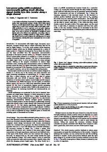
Spool Geometry and Design Parameters The geometry of our spool is presented in Fig. 5, which illustrates the central PWM section of our spool unwrapped from the spool surface. The helical barriers unfold into a triangular sawtooth partition. As the spool rotates, the helical barriers translate across the inlets and fluid is directed from one branch (application or tank) to the other. Note that the central PWM section of the spool is divided into N triangular sections corresponding to N inlets. Each triangular section performs one complete on/off cycle. Therefore, there are N PWM cycles per revolution of the spool and the PWM frequency of the valve is N times the spool frequency. A description of the relevant design parameters for the spool geometry is given in Table 1. The inlet orifice of our design is shaped as a rhombus with sides of length Rs that are parallel to the helical barriers, as shown in Fig. 5. A rhombus shaped inlet provides a faster rate of change in area ( dA dθ ) than a circular orifice of equal size during the initial and final stages of transition, which can be seen in Fig. 6. These are the regions where quick transitions are desirable since most throttling losses occur when the inlet orifice is just beginning to open or close. Note that the area gradient dA dθ is constant for a rhombus shaped inlet. Four transition events occur every PWM cycle in our 3-way design: opening and closing of the inlet to the load branch, and opening and closing to the tank branch. The proportion of time that the valve is in transition is dependent on the width of the rhombus inlet, Rw , thickness of the helical barriers, Ht , and the number of PWM sections on the spool surface, N. Thus, the proportion of time that the valve is in transition is:

energy loss due to fluid compressibility [6]. A diagram of our valve assembly is presented in Figs. 3 and 4. Figure 4 reveals a closer look at the interior geometry of our design as well as illustrates many of the design features.

κ= 3

  Ht 2 · N · Rw + sin(β) π·D

(1)

c 2007 by ASME Copyright

Parameter

Description

D

Spool diameter

R

Spool radius, R =

D 2

Ls

Spool length

L

PWM section length

Le

Exit section length

Rh

Rhombus height

Rw

Rhombus width

Rs

Rhombus side length, Rs =

1 2

β

Helix angle

Hh

Helix height

Hw

Helix width

Ht

Helix thickness

N

Number of helices Table 1.

outlet turbine exit area Aout (see Fig. 16) represent a direct tradeoff between the spool rotational velocity, valve transition time, and fully-open throttling losses. We define ∆Popen to be the pressure drop across the rhombus inlet when it is fully open, and ∆Pexit to be the pressure drop across the outlet turbine exit. When ∆Popen or ∆Pexit is large, more kinetic energy is transferred to the fluid resulting in a higher spool velocity. This speed, however, is attained at the cost of greater throttling losses. Ain and Aout are sized in our current design such that the fully open throttling losses do not exceed some maximum acceptable value. Since the flow rate Q of the system is constant, the maximum throttling loss requirement limits the pressure drop across the inlet and outlet stages, which determines Ain and Aout . The maximum fully open throttling loss is given by Power = (∆Popen + ∆Pexit ) · Q. Ain and Aout can be calculated using the orifice equation, which is defined as:

q

R2w + R2h

ρ ∆P = 2

x 10

Open Orifice Area (m2)

2

(2)

2.2

Linear Actuation and Sensing The axial position of the spool is actuated hydro-statically using an electro-hydraulic gerotor pump that is hydraulically connected to both ends of the valve sleeve. A schematic of the hydraulic axial position system is presented in Fig. 7. The DC motor is powered by a PWM controller H-bridge electrical circuit. By pumping fluid from one end of the sleeve to the other, the axial position of the spool can be varied. The gerotor pump flow rate is statically related to the input to the DC motor driving circuit. The hydraulic axial control system was chosen for its elegance as well as its simplicity. The axial position of the spool is measured using a noncontact optical method. A sensor plate with two LEDs and a photodiode is mounted to one end of the valve sleeve. The light emitted from the LEDs is reflected off of the surface of the valve spool and sensed by a photodiode in the sensor plate. The light intensity detected by the photodiode decreases as the distance between the photodiode and spool surface increases. Therefore the position of the spool can be measured from the output voltage of the photodiode.

1.2 1 0.8 0.6 0.4 0.2 0 0

Q Cd · A · N

ρ is the density of hydraulic oil, Cd is the orifice discharge coefficient, and A is the cross-sectional area of interest. The height, Rh , and width, Rw , of the rhombus are constrained by the inlet area according to Ain = .5 · Rw · Rh .

Definition of parameters

−5

1.4



Circle Rhombus 0.1

Figure 6.

0.2

θ (rad)

0.3

0.4

0.5

Open orifice area during transition

0 ≤ κ ≤ 1. Physically, Rw is constrained such that 0 ≤ κ ≤ 1 while Rh is constrained by the length of the PWM section of the spool, or Rh < L. Ideally, κ must be small to minimize the proportion of each PWM cycle that the valve is in transition. Since our valve is least efficient during transition, decreasing κ will increase the efficiency of our valve. κ can be decreased by setting Rw to be small, or D to be large. Both cases, however, increase the surface area of the spool, which increases viscous friction and decreases the spool velocity. The sizing of the rhombus shaped inlet orifice area Ain and

2.3

Rotary Sensing The rotary sensing of the spool is achieved similarly to the linear sensing. The rotary position and angular velocity of the spool are measured using a 32 sector code wheel that is attached 4

c 2007 by ASME Copyright

Figure 9.

Change in rhombus area during transition

−5

1.4

x 10

Figure 7.

Open Orifice Area (m2)

1.2

Diagram of linear actuation and rotary sensing system

1 0.8 0.6 0.4 0.2 0 0

Load Branch Tank Branch 0.5

Figure 10.

Figure 8.

1

θ (rad)

1.5

2

2.5

Open orifice area for 1 PWM period

the valve. This section is organized as follows: Section 3.1 provides an analysis of the throttling losses experienced by our valve, while Section 3.2 presents the relationship between the spools’s axial position and flow. Section 3.3 contains a method of estimating the spool velocity and Section 3.4 provides an analysis on the effect bearing surface area on viscous friction. A preliminary leakage analysis is presented in Section 3.5, and a summary of our design is given in Section 3.6.

Circuit diagram of PWM variable displacement pump

to one end of the spool. A low-power diode laser module and a photodiode are mounted on a sensor plate, which is attached to one end of the sleeve. The intensity of the reflected light varies significantly with the position of the code wheel. This light intensity is detected by the photodiode and is transformed into a proportional voltage signal. A counter is used to store the voltage information, from which the spool velocity can be calculated. A reference is added to one sector to reset the counter for determining the spool’s axial position.

3.1

Valve Throttling Losses Our valve experiences two types of throttling losses: constant (or fully open) losses that occur across the rhombus inlets and outlet turbine exits, and transition losses that occur as the valve opens and closes to application and tank. The regions where these two losses occur during each PWM cycle is illustrated in Fig. 11, which corresponds to the area plots shown in Fig. 10. Figures 13 and 12 illustrate the pressure drop across the inlet and flow profiles corresponding to Fig. 10. The total throttling power loss for one PWM cycle can be found by multiplying the curves in Figs. 12 and 13 together. The result is shown in Fig. 14, which reveals that a majority of the energy loss occurs during transition when the relief valve opens and during the two

3 Throttling Loss and Flow Analysis The analysis presented in this section is based upon the system shown in Fig. 8. The system consists of an ideal flow source with flow rate Q, relief valve set at Prelie f , and a constant application or load pressure of Pload . An orifice load will be considered in the simulation discussed in Section 4. Pin is defined as the pressure in the inlet volume, which is the volume upstream of 5

c 2007 by ASME Copyright

Power Loss (W)

6

x 10

5000 Load

8

Prelief 7

Pload+Popen

Transition losses

4 Fully open losses 3

1 Popen 0.5

Figure 11.

Load branch Tank branch Relief valve

θ (rad)

1.5

2

2.5

0.5

1

1.5

2

2.5

0.5

1

1.5

2

2.5

5 0 0 −4 x 10

0 0

0.5

Figure 12.

6

x 10

1

θ (rad)

1.5

2

2.5

Flow rate through valve for 1 PWM period

Pressure Drop Across Orifice (Pa)

4 2 0 0

0.5

1

1.5

2

1

1.5

2

2.5

0 0 5000

0.5

1

1.5

2

2.5

0 0

0.5

1

1.5

2

2.5

θ (rad)

Transition power loss for 1 PWM period

2.5

6

Tank Branch

0.5

(3)

During transition, throttling losses occur because the valve cannot open and close instantaneously. As a result the inlet orifice is partially open during transition, which induces a large pressure drop across the orifice. To estimate the throttling losses of our valve during transition, we neglect the short period during the transition when the inlet orifice is simultaneously open to both load and tank. Assuming that the spool rotates at a constant angular velocity ω, we expect the transition time for each transition event to be equal and given by:

6

8

0 0 5000

Poweropen = (1 − κ) · (∆Popen + ∆Pexit ) · Q

5

8

2.5

tank transition events. The first type of loss, the fully open loss, is determined by the sizing of Ain and Aout as described in Section 2.1. The fully open loss is estimated by assuming that the full system flow Q enters and exits the valve throughout the entire PWM cycle when the valve is not in transition. As shown in Fig. 11, we only consider the fully open losses to occur when the valve is not transitioning. The losses that occur across Ain and Aout during transition will be included in the transition losses. Thus, the fully open losses can be estimated by considering ∆Popen , ∆Pexit , Q, and κ:

5

0 0 −4 x 10

2

Figure 14.

Inlet pressure for 1 PWM period Flow Rate (m3/s)

−4

x 10

Load branch

1

1.5

Total

2

0 0

1

Tank

5

0.5

Relief

Inlet Pressure (Pa)

6

0 0 5000

ttrans = 2 ·

x 10

Ht Rw + sin(β)

D·ω

!

(4)

6 4

Since ttrans is constant, we expect the energy lost during the two transition events involving the load branch (opening and closing) to be equal, and similarly for the two events involving the tank branch. We define ∆Pon and Qload to be the pressure drop and flow though the open orifice area Aopen when the valve is connected to the load branch, and similarly define ∆Po f f and Qtank

2 0 0

Figure 13.

0.5

1

θ (rad)

1.5

2

2.5

Pressure drop across inlet orifice for 1 PWM period

6

c 2007 by ASME Copyright

for when the valve is connected to tank. Aopen is a function of the spool’s angular position θ, and is determined from geometry to be: Aopen (θ) = Rs · R · sin(β) · θ

that the inlet pressure is now the pressure drop across the orifice ∆Pon plus the load pressure. When the relief valve is open, flow is throttled across Prelie f through the relief valve, but only across (Prelie f − Pload ) through Aopen . We now consider the transition when the orifice is beginning to open to the load branch. The energy lost during the initial stage of the transition when the relief valve is open is:

(5)

We now consider the throttling losses during the two transitions to tank. When the inlet orifice is opening, the initial inlet pressure is high and the relief valve is open. As the open orifice area increases, the pressure begins to decrease until the relief valve closes and the full flow Q is sent through the valve to tank. Initially, when the relief valve is open, the inlet pressure is fixed at Prelie f and flow is being throttled across both the relief valve and inlet orifice area Aopen . During this period, flow is throttled across both the relief valve and Aopen at a pressure drop of Prelie f . Thus, the energy lost while the relief valve is open is: Etrans,1 =

Z t=tR t=0

Q · Prelie f dt

1 θ=θR (Q − Qload ) · Prelie f · dθ ω θ=0 Z 1 θ=θR + Qload · (Prelie f − Pload ) · dθ ω θ=0 s   Popen 1 Q · Rw (9) · · Prelie f − Pload = ω·R (Prelie f − Pload ) 2 Z

Etrans,3 =

Once the relief valve closes, the remaining energy loss during the transition is:

(6)

tR is the time when the pressure at the inlet is equal to Prelie f and the relief valve is on the verge of closing. We now use the definition of ω = dθ dt to integrate Eq. 6 with respect to θ: 1 θ=θR Q · Prelie f · dθ ω θ=0 Q · Rw p · Popen · Prelie f = ω·R

Etrans,1 =

Z

1 θ= R Q · ∆Po f f · dθ ω θ=θR Q · Rw q · Popen · (Prelie f − Popen ) = ω·R Z

Z θ= Rw R θ=θR

(10)

The total energy lost during the transition from fully closed to fully open to the load branch is the sum of Eq. 9 and Eq. 10. The total energy lost for all four transition events, or for one complete PWM cycle, is:

(7)

θR is the angular displacement corresponding to the orifice area that produces Prelie f . At θR , the relief valve closes as the inlet pressure just begins to fall below Prelie f . θR can be calculated using the orifice equation, Eq. 2, and Eq. 5. Once the inlet pressure drops below Prelie f and the relief valve closes, the flow through Aopen is Q and remains constant for the remainder of the transition. ∆Po f f , the pressure drop across the orifice, is calculated using the orifice equation. The energy loss for the remainder of the transition with the relief valve closed is:

Etrans,2 =

1 ω

Q · Pon · dθ s ! (Prelie f − Pload ) Q · Rw · Popen · −1 = ω·R Popen

Etrans,4 =

Etrans,total = 2 · (Etrans,1 + Etrans,2 + Etrans,3 + Etrans,4 )

(11)

The total power loss due to fully open and transition throttling is: Powertotal = Poweropen + Etrans,total · N ·

ω 2·π

(12)

3.2

Output Flow vs. Axial Position The relationship between flow to the load and tank branches with respect to the axial displacement was determined numerically using the Matlab model presented in Section 4. The results are shown in Fig. 15. The central portion of Fig. 15 is linear, which is expected given the linear nature of the helical barrier shown in Fig. 5. Toward the two extremes of the axial travel the flow levels off. This is when the full flow is directed to either load or tank and the inlet does not overlap the barriers at all. In between the linear and level portions of the curve exist nonlinearities, which occur due to the junctions where the barriers intersect. Note that Qload + Qtank 6= Q due to flow through the relief

Rw

(8)

The total energy lost during the transition from fully closed to fully open to tank is the sum of Eq. 7 and Eq. 8. The energy loss during the two transitions involving the load branch are calculated in a similar manner. The main difference is 7

c 2007 by ASME Copyright

1.4 1.2

Load Branch Tank Branch Load+Tank

6

Pload=2.1 × 10 Pa

Normalized Flow

1 0.8 0.6 P

0.4

=6.9 × 106 Pa

load

0.2 0 0

Figure 15.

0.2

0.4 0.6 Normalized Axial Travel

0.8

1

Relationship between flow and axial position

valve during transition. Also note that Qload decreases as Pload increases, which is expected since the relief valve opens for a greater proportion of transition for a higher load pressure. This is because Pin = ∆Pon +Pload ≤ Prelie f . The total flow, Qload +Qtank , in the linear range of the axial travel between 20% − 80%, is especially low (about 90%) due to the relief valve opening during transition, which indicates a significant source of energy loss. Methods to reduce or eliminate the energy lost through the relief valve must be investigated.

Figure 16.

is the effective surface area of the spool. The Ae f f is estimated numerically in Section 3.4 using a simple CFD analysis. In our current design, the inlet stage of the valve spool has the functionality of an impulse turbine, and the outlet stage a reaction turbine [4]. A sketch of the inlet and outlet stages of the valve as well as the control volumes that were used is shown in Fig. 16. The inlet stage of the valve consists of N stationary inlet nozzles located on the valve sleeve tangential to the spool. The inlets are offset a distance Rin from the center of the spool. In the inlet stage analysis, we consider a stationary control volume that surrounds the spool and inlets. This control volume has N inlets and one outlet, although for simplicity, only one inlet is shown in Fig. 16. At the inlets, angular momentum is generated in the fluid as it enters the control volume tangentially. Since the fluid exits the control volume through an internal axial passage, we assume that the fluid exits with no angular momentum, and that all of the angular momentum generated by the inlets is transferred to the spool. Using this control volume approach, the torque generated by the inlet stage is:

3.3

Spool Velocity Analysis The spool rotational velocity was calculated by considering an angular momentum balance on the spool. The analysis assumes incompressible flow and one-dimensional inlets and outlets. The momentum balance yields: J · θ¨ = τin + τout − τ f

(13)

J is the mass moment of inertia of the spool and θ¨ is the angular acceleration of the spool. τin is the torque generated by the inlet stage turbine, and τout by the outlet stage. In the steady state, θ¨ = 0 and the angular momentum generated by the inlet and outlet stages of the spool are balanced by viscous friction. The resistive torque due to viscous friction was assumed to obey Petroff’s Law. Petroff’s Law presumes that the torque due to friction is proportional to the bearing surface area, shear stress, and the moment arm where the shear stress acts on the system [3]. Thus, the torque due to friction is given by: τ f = Ae f f ·

µ 2 ·R ·ω c

Sketches of the inlet and outlet turbine stages

N

τin = ∑(Rin × v)in · m˙ in = 1

ρ · Rin · Q2 Ain · N

(15)

ρ is the density of hydraulic oil, v is the mean velocity of the fluid as it exits the inlet nozzle, and m˙ is the mass flow rate through the nozzle.

(14)

R is the spool radius, µ is the dynamic viscosity of hydraulic oil, c is the radial clearance between the spool and sleeve, and Ae f f

By equating τin = τ f , the velocity of the spool generated by 8

c 2007 by ASME Copyright

the inlet stage alone is: ω=

ρ · Q2 Rin · N · R2 · Ae f f · µc Ain

(16)

The outlet stage of the valve consists of N curved blades that turn the flow as is travels outward. In the outlet stage turbine analysis, we consider a control volume that rotates with the spool. This control volume consists of one inlet, and N rotating outlets, although only one is shown for simplicity in Fig. 16. Fluid enters the outlet stage axially through the internal axial passage which connects the inlet stage to the outlet stage. Since the fluid enters the stage axially, it is assumed to have no angular momentum as it enters the control volume. As the fluid is directed outward and tangential to the spool surface, a reaction torque is experienced by the spool as it turns the flow. The outlet stage is assumed to be ideal such that the fluid is completely turned by the blades. With this assumption, the outlet stage can be thought of as a rotating tangential outlet nozzle with area Aout = cout · Le offset a distance Rout from the center of the spool. The torque generated by the outlet stage is:

Figure 17.

expense of pressure drop) will increase the spool velocity. The momentum generated by the outlet, however, is counteracted by 2 the additional RRout 2 · ρ · Q term, which corresponds to the angular momentum which must be transferred to the fluid as it is forced to rotate with the same circumferential velocity as the outlet blades. As the fluid flows radially outward, more momentum must be transferred to the fluid as the circumferential velocity of the outlet blades increases proportionally with Rout . Therefore, increasing the outlet moment arm Rout also has the effect of decreasing the spool speed. The greatest benefit from the addition of the outlet stage turbine is that the effects of the inlet geometry on the PWM functionality of the valve can be decoupled from the spool velocity. By using the outlet stage to provide a majority of the momentum to rotate the spool, the inlet orifice area and thickness of the helical barriers can be optimized for PWM. The only potential issue is whether or not the outlet stage can be designed as effectively as the inlet stage, which resembles the more traditional inflow turbine geometry.

ρ · Rout 2 ·Q −R2out ·ρ·ω·Q A · N out 1 (17) vCV = Rout · ω is the velocity of the control volume. Equating the inlet and outlet torque to the friction torque in the steady state produces the equation for ω, the angular velocity of the spool generated by both stages: N

τout = ∑(Rout ×(v−vCV ))out · m˙ out =

ω=

ρ · Q2 N · R2 · (Ae f f

µ c

· +

R2out R2

Rin · ρ · Q) A ·

(18) 3.4

Effective Bearing Surface Analysis A simple CFD analysis was performed to calculate the effective bearing surface area of the spool. The effective surface area accounts for the contribution of the non-bearing surface area to the friction torque. The non-bearing surface area is defined to be the total surface area π · D · L minus the bearing surface area, which is shown in Fig. 17. Ae f f is given by:

From Eq. 18, we see that the combined inlet and outlet effects can be normalized such that the system resembles an inlet only configuration. A is defined as the equivalent area, and is given by: Rout 1 1 + = A Ain Rin · Aout

Bearing surface area of valve spool

Ae f f = Abearing + α · (π · D · Ls − Abearing )

(19)

(20)

α is defined to be the ratio of non-bearing shear stress to bearσ ing surface shear, or α = non−bearing σbearing . The objective of our CFD analysis is to determine α. In our current design, the radial bearing surface area clearance is 2.54×10−5 m while the radial clearance for the remaining surface area is 3.175 × 10−3 m. Petroff’s Law, which assumes a Newtonian fluid where shear stress is inversely proportional to

Note that setting Rout = 0 reduces Eq. 18 to the inlet turbine only case. Eq. 18 illustrates the dual effects of the outlet stage turout bine on the spool velocity. RinR·A corresponds to the angular out momentum generated by the tangential outlet. Either increasing the moment arm Rout or decreasing the outlet nozzle area Aout (and thereby imparting more kinetic energy to the fluid at the 9

c 2007 by ASME Copyright

−3

x 10 5

Pocket depth (m)

4

Figure 18.

3 2 1 0

Schematic of pocketed non-bearing surface

−1 −2

clearance, would predict that the effect of the non-bearing area is negligible. Our previous experiments with a .0323m diameter rotary valve, however, revealed otherwise. This is because the fluid in contact with the non-bearing surface area is trapped in a pocketed area between the helical barriers. The fluid in the pocket will recirculate due to the no-slip conditions at the outer stationary sleeve wall as the spool rotates. These vortices will increase the frictional force in the pocketed area. In our current design, however, the fluid is not completely trapped between the helical barriers. The inlets between the barriers direct fluid toward the center of the spool. Therefore, we expect less circulation and vorticity in our current design, which should correspond to less friction in the non-bearing surface area. Thus the following analysis is a conservative prediction of what the non-bearing friction will be. A diagram of a simplified model of the pocketed area is shown in Fig. 18. Although the actual upper boundary of the domain is curved (sleeve ID) as shown in Fig. 18, we will approximate the upper surface as flat to simplify the analysis. As a further simplification, the system is inverted. Instead of rotating the spool in the simulation, we rotate the sleeve. In the computational domain, this equates to a moving upper boundary. The CFD analysis assumes two-dimensional, steady, incompressible Newtonian flow. The pocket was modeled as a rectangular chamber with a moving upper boundary. The upper boundary was given a velocity that corresponded with our previous valve, a .0323m diameter spool rotating at 27Hz. Both the depth and width of the pocketed area were explored. A plot of the streamlines generated by the CFD code illustrating the primary vortex of the flow is shown in Fig. 19. The primary vortex accounts for the circulation occurring within the pocket between the helical barriers. The numerical results of the analysis are presented in Figs. 20 and 21. These figures show that the width of the pocket has a negligible effect on the shear stress, while the depth of the pocket is crucial. Therefore, in our current design, we will design the pocket depth, or clearance of the non-bearing area, to be as large as possible while still maintaining adequate wall thickness for the internal axial passage between the inlet and outlet stages. From Fig. 20, for a depth of 3.175 × 10−3 m, the corresponding

1

2

3

4 5 6 Pocket width (m)

Figure 19.

7

8

9 −3

x 10

Streamlines within pocket

Pocket Width = 9.525 × 10−3 m 850 800

Shear Stress (N/m2)

750 700 650 600 550 500 450 400 2

4

Figure 20.

6

8 10 Pocket Depth (m)

12

14 −3

x 10

Effect of pocket depth on shear stress

shear stress is predicted to be roughly 820N/m2 = σnon−bearing . The shear stress for the bearing surface of a .0323m diameter spool rotating at a frequency of 27Hz with a radial clearance of 2.54 × 10−5 m results in σbearing = 4169N/m2 . Therefore, σ α = non−bearing σbearing = 19.7%.

3.5

Leakage Analysis

A preliminary analysis of the internal leakage of the valve was conducted by assuming laminar leakage flow. Since the only feature of the valve that separates high pressure fluid from low pressure fluid is the helical barrier, the valve leakage is assumed to be the flow across this area. The following equation was used 10

c 2007 by ASME Copyright

Shear Stress (N/m2)

Pocket Depth = 3.175 × 10−3 m 850

Parameter

SI

English

Description

800

N

3

−

Number of inlets

750

D

.0254m

1.0in

Spool diameter

700

L

.0856m

3.37in

Spool length

c

2.54 × 10−5 m

.001in

Radial clearance

α

.197

-

Ratio of shear

Abearing

.0015m2

2.39in2

Bearing area

Ain

1.22 × 10−5 m2

.0189in2

Inlet rhombus area

Aout

4.68 × 10−5 m2

.0726in2

Turbine exit area

Rh

.0065m

.2558in2

Rhombus height

Rw

.0037m

.1476in2

Rhombus width

β

1.05rad

60deg

Helix angle

Ht

.003m

.1181in

Helix thickness

Cd

.6

-

Orifice coefficient

Q

6.3 × 10−4 m3 /s

10gpm

Flow rate

Pload

6.89 × 106 Pa

1000psi

Load pressure

Prelie f

7.58 × 106 Pa

1100psi

Relief pressure

650 600 550 500 450 400 2

4

Figure 21.

6

8 10 Pocket Width (m)

12

14 −3

x 10

Effect of pocket width on shear stress

to estimate the leakage [5]:

Qleak =

Per · c3 · (Pload

− Popen ) (12 · µ · Ht )

(21)

Per is the perimeter of the leakage surface. This equation indicates a strong relationship between the leakage and the clearance. A small clearance is desirable to reduce leakage, however a small clearance increases the viscous friction drag on the spool and reduces the spool velocity.

Table 2.

Current system design parameters

Our current prototype is sized for a nominal flow rate of 40l/m at a maximum operating pressure of 7M pa. The design goals for our valve are to maximize the spool velocity, and minimize losses and physical size. Based on the analysis presented in this paper as well as considering manufacturing constraints, the final parameters chosen for our first prototype are summarized in Table 2. From our current design parameters, we predict that our spool can achieve a rotational velocity of 28Hz, which corresponds to a PWM frequency of 84Hz. This is a conservative estimate since we believe our estimate of α from the CFD analysis is an over prediction. κ, the proportion of time per revolution that the valve is in transition, is 54.2%. The resisting torque due to viscous friction is estimated to be 0.1116N/m. From this we estimate that an input power of 19.6W is needed to overcome viscous friction. The pressure drop across the fully open rhombus inlet and outlet turbine exit are 3.6275 × 105 Pa and 2.4541 × 104 Pa respectively. The leakage flow across the helical barriers is 1.2618 × 10−5 m3 /s and the total energy lost per PWM cycle due to transition throttling is 13.6J. Therefore, the total power loss attributed to our valve, which consists of transition and fully open throttling, is 1256W . The total power loss can be expressed as an equivalent pressure drop, which is

3.6

Design Summary Several trade offs exist in the design of our self-spinning, 3-way rotary valve concept. By specifying L and D, the optimal rhombus inlet area becomes constrained by Aκin2 = π·D·L 48·N . By decreasing Ain , κ must decrease as well, which indicates that the valve is in transition for a smaller proportion of each PWM cycle. This equates to higher efficiency since our valve is least efficient during transition. Additionally, from Eq. 18, the rotational speed of our valve ω also increases with a smaller Ain . Decreasing Ain , however, increases the fully open throttling losses across the inlet, which is a constant loss throughout each rotation of the spool. If we wish to decrease the transition losses at the inlet by manipulating Ain , ω can be maintained by appropriately specifying Aout . Another trade off in our design exists between leakage across the helical barriers and ω. A smaller radial clearance c significantly decreases leakage, however the penalty in spool velocity is significant as well. The PWM frequency of our design is proportional to the spool velocity by a factor N. By increasing N, the PWM frequency of our valve can be increased for a given ω. However, N is limited by leakage, as the thickness of the barriers Ht must decrease with N. 11

c 2007 by ASME Copyright

equal to 1.99 × 106 Pa. Compared to the maximum output power of our system, Powerout = Q · Pload = 4350W , the system efficiency is 71.1%. This estimated system efficiency includes the energy required to drive the valve; no additional power source is required. From the analysis presented in this paper, the majority of power loss is due to throttling during transition. In our 3-way valve configuration, the transition losses are especially high since the number of transition events is doubled in comparison to a 2way valve. The additional transition losses incurred by the 3-way design, however, are offset by the enhanced self-spinning capability. A 2-way valve requires an auxiliary power source to spin the valve during the portion of the PWM cycle when there is no flow through the valve. Additional complications arise when coupling an outside power source to the valve spool. Furthermore, transition throttling losses are not unique to our rotary valve, and exist for any on/off valve. Additional investigation into the role of the inlet geometry on the transition loss can potentially decrease losses as our current inlet was designed by considering the fully open losses only.

6

7

p Pre f + K f b · (Pre f − Pout (t))

Pressure (Pa)

5 4 3 2 1 0 0

0.5

Figure 22.

1

1.5 Time (s)

2

2.5

3

Simulated output pressure

u is the input to the DC motor PWM driving circuit, l is the axial position of the spool, and Aend = π4 · D2 is the area of one end of the spool. A PI controller with feedforward is used to track l to a reference signal. The system poles were placed at −10rad/s and −15rad/s. Simulations of the axial position controller predict that the controller can reposition the spool from full on to full off in less than .15s. A step reference pressure from 1.3789 × 106 Pa to 5.52 × 106 Pa with a second step to 3.45 × 106 Pa was simulated. This input corresponds to a step in flow from 1.99 × 10−4 m3 /s to 3.97 × 10−4 m3 /s to 3.15 × 10−4 m3 /s. The system was able to complete the first step in .19s and the second step in .054s. The average pressure ripple was 6.67%. The results of the simulation are presented in Figs. 22 and 23, and show that our 3-way rotary valve with hydro-static linear actuation can work effectively to modulate flow. The response of the simulated system is currently limited by the accumulator. The speed of the system can be increased by either decreasing the pre-charge pressure, or decreasing the precharge volume of the accumulator. Either of these modifications, however, will increase the magnitude of the output pressure ripple. Another alternative is to increase the PWM frequency of the system. This can further improve the response without the penalty in ripple size.

(22)

s(t) is the desired duty ratio and Pre f is the desired reference output pressure. K f b , the feedback gain, was chosen to be .01, which provided a good compromise between responsiveness and overshoot. K f f , the feedforward gain, was calculated to be 2.69 × 10−4 based on an orifice load. The relationship between duty ratio, s(t), and the axial position of the spool, l, is given in Fig. 15. Inverting the load branch curve in Fig. 15 produces the relationship for calculating the axial position as a function of duty ratio. The axial position of the spool corresponding to the desired duty ratio is regulated by controlling the input to a DC motor PWM driving circuit. The input is given by: f (u) l˙ = Aend

Reference Output

6

4 Rotary Valve Simulation A dynamic model of the system shown in Fig. 8 was simulated in Matlab. The system consists of an ideal flow source with a constant flow rate of 6.31 × 10−4 m3 /s and an ideal relief valve set at 7.58 × 106 Pa. The accumulator is assumed to be adiabatic with a pre-charge pressure of 6.89 × 105 Pa and a pre-charge gas volume of .16L. An orifice load described by Eq. 2 with a diameter of 0.0025m and discharge coefficient of .7 was used in the model. The current model assumes no fluid compressibility. The complete system is controlled using a pressure control algorithm proposed by Li et al. [7] of the form: s(t) = K f f ·

x 10

5 Conclusion A novel 3-way self-spinning rotary on/off valve concept has been presented that is potentially more efficient than a comparable linear valve of equal switching frequency and flow rating. The analysis in this paper predicts that a rotary valve sized for a nominal flow rate of 40l/m can achieve a PWM frequency of 84Hz, roughly a 400% improvement over current linear valve de-

(23) 12

c 2007 by ASME Copyright

REFERENCES [1] H. Merritt, Hydraulic Control Systems. John Wiley and Sons, 1967. [2] F. White, Fluid Mechanics. McGraw-Hill, 5th ed., 2003. [3] A. Cameron, Basic Lubrication Theory. John Wiley and Sons, 3rd ed., 1981. [4] S.L. Dixon, Fluid Mechanics and Thermodynamics of Turbomachinery. Elsevier Butterworth-Heinemann, 5th ed., 2005. [5] J. Cundiff, Fluid Power Circuits and Controls. CRC Press, 2002. [6] M. Rannow, H. Tu, P. Li and T. Chase, “Software Enabled Variable Displacement Pumps - Experimental Studies” Proceedings of the 2006 ASME-IMECE, no. IMECE2006-14973, 2006. [7] P. Li, C. Li and T. Chase, “Software Enabled Variable Displacement Pumps” Proceedings of the 2005 ASME-IMECE, no. IMECE2005-81376, 2005. [8] S. Yokota, Y. Kondou and K. Akutu, “Ultra fast-acting electro-hydraulic digital valve by making use of a multilayered piezo-electric device (PZT),” Proceedings of Flucome’ 91, pp. 379–384, 1991. [9] T. Kajima, S. Satoh and R. Sagawa, “Development of a high speed solenoid valve,” Transactions of the Japan Society of Mechanical Engineering: Part C, vol. 60, no. 576, pp. 2744– 2751, 1994. [10] H. Lu, C. Zhu, S. Zeng, Y. Huang, M. Zhou and Y. He, “Study on the new kind of electro-hydraulic high speed onoff valve driven by PZT components and its powerful and speedy technique,” Chinese Journal of Mechanical Engineering, vol. 38, no. 8, pp. 118–121, 2002. [11] I. Cyphelly and J. Langen, “Ein neues energiesparendes Konzept der Volumenstromdosierung mit Konstantpumpen” Aachener Fluidtechnisches Kolloquium, 1980. [12] T. Royston and R. Singh, “Development of a Pulse-Width Modulated Pneumatic Rotary Valve for Actuator Position Control” Journal of Dynamic Systems, Measurement, and Control-Transactions of the ASME, vol. 115, pp. 495–505, 1993. [13] P. Cui, R. Burton and P. Ukrainetz, “Development of a high speed on/off valve,” Transactions of the SAE, vol. 100, no. 2, pp. 312–316, 1991. [14] Industrial Hydraulics Manual. Eaton Corporation, 4th ed., 2001.

−4

5

x 10

Output Flow (m3/s)

4.5 4 3.5 3 2.5 2 1.5 0

0.5

1

Figure 23.

1.5 Time (s)

2

2.5

3

Simulated output flow

signs. This frequency is attained by harvesting waste throttling energy from the system flow. No external actuation is needed to rotate the spool in this design. A complete system model of a PWM variable displacement pump utilizing our 3-way rotary valve has been simulated with promising results. The simulation shows that the hydro-static linear control scheme is effective in controlling the axial position of the spool. The simulation also shows that variable displacement pump functionality utilizing the rotary valve can be achieved by adding closed-loop control to the system. A number of trade offs between performance and efficiency exist in the design of our rotary on/off valve. The equations presented in this paper provide a means for sizing and optimizing the design based upon physical constraints and efficiency requirements. An analysis of the various modes of power loss in the system reveal that throttling during transition accounts for a majority of the loss in our valve. An opportunity exists to reduce transition losses by optimizing the valve geometry to transition more effectively. κ, the proportion of time that the valve is in transition, needs to be reduced to improve efficiency. This can be achieved by decreasing Rw , increasing D, or by having the valve spin selectively faster during transition. Reducing or eliminating the flow throttled across the relief valve during transition will improve efficiency significantly as well. Our design can also be improved by investigating methods of decreasing viscous friction, increasing the number of helical barriers (N), as well as developing a more effective outlet stage turbine.

Acknowledgment This material is based upon work supported by the National Science Foundation under grant numbers ENG/CMS-0409832 and EEC-0540834. 13

c 2007 by ASME Copyright