Hybrid Booleans - Computer Graphics and Multimedia - RWTH-Aachen

Volume xx (200y), Number z, pp. 1–12

Hybrid Booleans Darko Pavi´c and Marcel Campen and Leif Kobbelt RWTH Aachen University

Abstract In this paper we present a novel method to compute Boolean operations on polygonal meshes. Given a Boolean expression over an arbitrary number of input meshes we reliably and efficiently compute an output mesh which faithfully preserves the existing sharp features and precisely reconstructs the new features appearing along the intersections of the input meshes. The term "hybrid" applies to our method in two ways: First, our algorithm operates on a hybrid data structure which stores the original input polygons (surface data) in an adaptively refined octree (volume data). By this we combine the robustness of volumetric techniques with the accuracy of surfaceoriented techniques. Second, we generate a new triangulation only in a close vicinity around the intersections of the input meshes and thus preserve as much of the original mesh structure as possible (hybrid mesh). Since the actual processing of the Boolean operation is confined to a very small region around the intersections of the input meshes, we can achieve very high adaptive refinement resolutions and hence very high precision. We demonstrate our method on a number of challenging examples. Categories and Subject Descriptors (according to ACM CCS): Computer Graphics [I.3.5]: Computational Geometry and Object Modeling—

1. Introduction Creating a complex model by using a combination of simple primitives is one of the common paradigms in Computer Aided Geometric Design (CAGD). The used primitives can be as simple as spheres, cylinders and cubes, but arbitrarily complex solids could be used as well. The combination is usually described by a composition of so-called Boolean operations: unions, intersections and differences. Boolean operations are used in geometry processing not only for modeling, but also for simulation purposes. One example is the simulation of manufacturing processes such as milling and drilling. Moreover, one can use Boolean operations for collision detection, e.g., in order to check the validity of a specific configuration of a mechanical assembly. The evaluation of a Boolean expression can be described by a tree of the corresponding Boolean operations used in the expression, which is an approach well-known as Constructive Solid Geometry (CSG) [Req80, Man87]. On the one hand this representation is very simple and intuitive. Algorithms can be applied to CSG-models as if we had the boundary representation of the final model represented by the corresponding CSG expression. On the other hand the submitted to COMPUTER GRAPHICS Forum (10/2009).

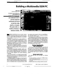
Figure 1: Boolean difference operation "Bunny–CGF". From left to right: visualization of the SURFACE cells after our adaptive refinement, the output mesh and two zoom-in views of the output showing the feature-sensitive extraction as well as the tesselation in the vicinity of the feature areas. Our method generates new geometry only in green areas whereas the rest is preserved from the input. CSG representation is not very effective, hence mainly for performance reasons one is interested in boundary model representations of the final result. Among all boundary representations for models in computer graphics the polygonal mesh is probably the most popular one. It has high approximation power, is very compact,

2

Darko Pavi´c & Marcel Campen & Leif Kobbelt / Hybrid Booleans

efficient and also hardware-accelerated. When computing Boolean operations on polygonal meshes the main problem encountered is the numerical stability. In order to avoid this problem the general approach in many applications is to first convert the polygonal mesh representation into a volumetric one. The polygonal mesh is rasterized and represented by a number of volume elements (=voxels). Then algorithms are applied to the volumetric representation, which is more robust. Finally, the polygonal solution is extracted from the volumetric result. In general this final extraction suffers from typical artifacts due to the limited voxel resolution. We present in this paper a novel, hybrid method for computing Boolean operations on polygonal meshes. The most important properties of our method are: • Hybrid representation and computations: We combine polygonal and volumetric representations and computations in order to achieve computational stability as well as high precision and efficiency. • Adaptivity: We use an adaptive octree data structure. The octree is refined only in the intersection areas of different input meshes. By this we generate a set of face-connected finest-resolution voxels only in a very small region within the bounding volume, which allows us to effectively work with very high voxel resolutions. • Structure preservation: During the hybrid extraction phase new geometry is generated only in the intersection areas of the given input meshes by using a wellestablished, robust volumetric approach. All parts of the input structure not affected by the Boolean combination are preserved and appropriately connected to the newly generated geometry. • Feature-sensitivity: Since we are preserving the input geometry where possible, most of the input features are naturally preserved. But also in the intersection areas of the given primitives we are able to properly extract sharp features. Because of our hybrid processing we are not directly limited by the voxel resolution. Hence we are also able to extract long and thin features occasionally created by Boolean combinations. In our case features are always meant to be geometric features, i.e. sharp edges or corners. Notice that there is also a different semantic notion of features in the area of solid modeling [SMN94]. In Fig. 1 we show an example for a difference operation between the bunny and a "CGF" model. Notice the highly adaptive refinement of our octree and the quality of the sharp features introduced in the output object. 2. Related Work The methods for computing Boolean operations can be distinguished based on three main properties: the type of input

data, the type of computation (e.g. volumetric or polygonal) and the type of output data. Early methods compute Boolean operations on boundary representations explicitly [RV85, ABJN85, LTH86, Car87, BN90]. Difficult case differentiations are introduced in order to capture all possible intersection cases between input elements (faces, edges, vertices). Some of these methods use adaptive octree structures like polytrees [Car87] or extended octrees [ABJN85, BN90] but mainly as a searching structure for faster access to needed elements. These polygonal algorithms in general suffer from numerical problems and although there is a number of ways to approach these problems [Hof01] for robustness reasons often volumetric methods are preferred. Keyser et al. [KCF∗ 02] have described a system for Boolean operations on curved solids which is completely based on exact arithmetics. They show that using exact arithmetics can be done in acceptable times in practice, but using floating point arithmetics is still one or two orders of magnitude faster. Computing Boolean operations on implicit surfaces corresponds to an appropriate application of min/max operations on the input distance fields. Museth et al. [MBWB02] have introduced a framework for editing operations on level set surfaces. Ho et al. apply their Cubical Marching Squares [HWC∗ 05] to extract Booleans from volume data. Varadhan et al. [VKZM06, VKSM04] have shown how to reliably extract a topology-preserving surface of a Boolean combination of given implicit surfaces. Their approach also allows for capturing geometries below the voxel resolution just like our hybrid extraction method. In general, volumetric methods are very robust but not as accurate as the polygonal ones. Especially the feature extraction remains problematic. In contrary, our method combines polygonal and volumetric computations and representations and thus is robust and efficient at the same time. For polygonal computations we show how to avoid using exact arithmetics in our specific case and so maintain high performance. The polygonal representation is also exploited in order to extract sharp features. In some special cases we introduce the sharp features by using the method recently presented by Pavi´c and Kobbelt [PK08] in the context of offset surface generation. Chen and Cheng [CC08] describe a hybrid hole filling method where a mesh hole is first filled by a volumetric approach and then stitched to the original geometry. Bischoff and Kobbelt [BK05] have proposed a hybrid structure preservation method in the context of CAD mesh repair which is not directly applicable to computing arbitrary Boolean expressions. We adopt and extend their idea to create a hybrid method for Booleans. The main challenges are how to detect the problematic regions and the extraction of the new geometry. The surface extraction methods based on the Marching Cubes idea [LC87] are not able to extract sharp features directly, at best they can be approximated by extrapolation [KBSS01, HWC∗ 05]. Schaefer and Warren [SW05] submitted to COMPUTER GRAPHICS Forum (10/2009).

Darko Pavi´c & Marcel Campen & Leif Kobbelt / Hybrid Booleans

have presented a Marching Cubes approach on dual grids, which are aligned to features and thus improve the extracted feature quality by construction. When polygonizing an implicit surface Ohtake et al. [OBP02] have introduced an optimization method which is able to reconstruct sharp features. We base our volumetric extraction on a variant of Dual Contouring [BPK05] which in contrary to the original work [JLSW02] is guaranteed to extract manifold surfaces. Boolean operations on other input data types like freeform solids [BKZ01] or point-based models [AD03,XQL06] have also been introduced. Other methods are based on non-manifold topology [Wei86] and compute non-manifold Booleans [GCP91]. There are also methods presented mainly concerned about how to render Booleans in realtime [HR05]. Although all these methods deal with Boolean operations they are not directly related to our approach.

3

information, stored in each cell, should be considered in the extraction stage. For this we tag all triangle references as VALID and those which should be omitted during the extraction are tagged INVALID. Extraction Finally we apply our hybrid method for featuresensitive extraction of the output mesh (Section 6). We first detect the critical regions, where the polygonal information of the input geometry is non-trivial. Here the surface is extracted by Extended Dual Contouring (EDC) as proposed by Bischoff et al. [BPK05]. EDC is a variant of the Dual Contouring approach [JLSW02] guaranteed to produce a manifold output. In the non-critical areas, which are in general significantly larger, the original geometry is explicitly preserved and appropriately connected to the EDC surface. 4. Rasterization

3. Overview of our Algorithm The input to our method is an arbitrary number of polygonal meshes Mi , i ∈ 0, ..., n − 1 combined in a Boolean expression B (M0 , ..., Mn−1 ) by using one of the following three Boolean operations: union "∪", intersection "∩" or difference "−". Note that difference "−" can also be used as a unary operator representing the complement operation. For polygonal meshes this corresponds to simple flipping of the normal directions. The input meshes Mi must be consistent, i.e. they must be water-tight and they should have consistently oriented normals. In the case of small cracks and holes our method would still work if the chosen voxel size is sufficiently large, but in general we cannot guarantee correctness for broken meshes. In the case of inconsistently oriented normals, the correct normal orientation can be computed, e.g., by using a minimal spanning tree as proposed by Hoppe et al. [HDD∗ 92]. For simplicity reasons for the rest of the paper we assume that all input meshes are triangle meshes. Our method consists of three main processing steps: Rasterization In the first step we rasterize the volume occupied by the input meshes (Section 4). A highly adaptive refinement in the intersection regions of different meshes is applied on a single octree data structure, where each leaf cell in addition to its structural information like grid position and size, stores the polygonal and volumetric information of the input geometry. The polygonal information consists of references to triangles which intersect the cell. The volumetric information is a INSIDE/OUTSIDE/SURFACE labeling computed w.r.t. each mesh individually. Evaluation The second step is the evaluation of the given Boolean expression B (M0 , ..., Mn−1 ) (Section 5) based on the hybrid representation, where the final, volumetric labeling of the output object is computed. During this step we also determine which portions of the polygonal submitted to COMPUTER GRAPHICS Forum (10/2009).

During the rasterization we create a hybrid representation of the input meshes Mi with respect to the given Boolean expression B (M0 , ..., Mn−1 ). An adaptive octree is built storing the hybrid information in the leaf cells. The polygonal information consists of references to all triangles which intersect a cell. The volumetric information consists of n INSIDE/OUTSIDE/SURFACE labels, one for each input mesh. 4.1. Adaptive Refinement We create an adaptive octree up to the given maximal octree depth d by refining an octree cell as long as it is intersected by more than one input mesh. All references to triangles intersecting a cell are stored. This adaptive refinement leads to a configuration where the leaf cells are mostly not at depth d. During the refinement we propagate the triangle references through the octree, so that only the triangles of the parent cell are used for future intersection tests. The cell-triangle intersection test can be efficiently computed by using the separating axis theorem [GLM96]. In Fig. 2 the rasterization procedure is depicted on a 2D example. After the adaptive refinement in all further processing stages we always work on leaf cells only. Therefore for the rest of the paper we are referring to leaf cells as cells. 4.2. Seed Filling on Adaptive Octrees In order to compute the labeling with respect to an input mesh Mi we proceed as follows: First, all cells containing references to triangles from Mi are labeled SURFACE. Then the remaining unlabeled cells must be labeled as either INSIDE or OUTSIDE with respect to Mi . For this we propose the following seed filling procedure for adaptive octrees: W.l.o.g. we first conquer the OUTSIDE regions. For this all unlabeled cells in the 26-neighborhood of the SURFACE cells lying "outside" with respect to all normals of

4

Darko Pavi´c & Marcel Campen & Leif Kobbelt / Hybrid Booleans

L0 M0

L

M1 M0 ∩ M1

M1

M0

B (M0 , M1 ) = M0 ∩ M1

M1 L1

unlabeled

SURFACE OUTSIDE INSIDE

Figure 2: Rasterization and Evaluation. Two input meshes and a Boolean expression are given (upper left). Then our adaptive refinement is applied creating the octree structure (lower left). The proposed seed filling on the adaptive octree creates the mesh labelings L0 and L1 (middle) used to compute the final labeling L (upper right). the referenced triangles are used as initial seeds and labeled OUTSIDE. Then recursively all unlabeled cells in the 6-neighborhood are visited and labeled OUTSIDE. Notice that digital topology implies that for non-SURFACE voxels the 26-neighborhood applies. The propagation of the OUTSIDE label to the 6-neighborhood is still sufficient because the seeding is done in the complete 26-neighborhood of the SURFACE voxels. Once the outside regions are conquered all remaining unlabeled cells are labeled INSIDE. After the execution of the seed filling procedure for each input mesh Mi the correct labeling LCi ∈ {INSIDE, OUT SIDE, SURFACE} is determined for each cell C (see 2D example in Fig. 2). Notice that our seed filling allows for more than one connected INSIDE or OUTSIDE component to exist and therefore is not limited to specific input geometries. Actually, our seed filling enables the proposed refinement (Section 4.1), which could increase the number of connected INSIDE/OUTSIDE components. 5. Evaluation of the Boolean Expression The evaluation of the given Boolean expresM0 M1 M2 M3 sion B (M0 , ..., Mn−1 ) is in fact a combined processing of the vol∪ M2 ∪ M3 umetric and the polyg- M0 ∩ M1 ∩ onal information. The − final labeling LC is computed from the in(M0 ∩ M1 ) − (M2 ∪ M3 ) dividual labelings LCi Figure 3: CSG tree example. and the polygonal information relevant for the output object is gathered from the input meshes. These two processing lines (volumetric and polygonal) are executed in parallel such that (intermediate) results from the one can support the computations in the other one and vice versa. For the purpose of evaluation we use the corresponding CSG-tree. This tree is induced by the given Boolean expression where the leafs are the input

M0 − M1

M0

Figure 4: Simple constellation of two meshes M0 and M1 for two different Boolean operations. All surface parts which do not contribute to the compound object are tagged INVALID (dashed lines). In the upper example the current status of the red cells is additionally changed to OUTSIDE. meshes and the inner nodes correspond to the used Boolean operations. Each operation defines a binary connection in the CSG-tree (example shown in Fig. 3). The CSG-tree is traversed for each cell C in order to obtain the final labeling LC . During the traversal we compute the current INSIDE/OUTSIDE/SURFACE status at each inner node. This can be done by applying the rules of Kleene’s strong ternary logic [Kle52], where the three values "true", "false" and "unknown" and the operations "logical AND" and "logical OR" correspond to our INSIDE, OUTSIDE and SURFACE labels and further to operations "∩" and "∪", respectively. Notice that the difference operation A − B corresponds to A ∩ (−B). If the cell status turns out to be INSIDE or OUTSIDE at some inner node we want to indicate that all references to triangles of the input meshes that correspond to the leafs of this node’s subtree do not contribute to the output object. For this purpose all such references are tagged INVALID. Otherwise, if the current cell status turns out to be SURFACE at an inner node and additionally has already been SURFACE at both child nodes then the triangles of different objects A and B meet within the cell. However, often not all of them contribute to the actual compound object (see Fig. 4). In order to avoid bad sample placement and overshooting geometry in the extracted surface that might arise from these superfluous triangles we check for each triangle reference whether it should remain VALID or not. Intuitively a triangle should remain VALID in a cell if and only if at least a part of it contributes to the actual compound object surface within that cell. If all triangle references are set INVALID during the test explained below, the surface of the actual compound object obviously does not intersect the cell. Hence, the cell’s status is switched from SURFACE to INSIDE or OUTSIDE depending on the current operator, thereby improving the volumetric representation. To actually check the validity of a triangle t of object A we test it for intersection with the triangles of object B (Notice: Such intersection is a segment on the intersection line of the corresponding triangle supporting planes): submitted to COMPUTER GRAPHICS Forum (10/2009).

Darko Pavi´c & Marcel Campen & Leif Kobbelt / Hybrid Booleans

object A

nk

5

object B

1

ej ej+1 v

q v p

nk+1

2

ej+2

p

1

(a) (b) Figure 5: (a): Determination of a visible triangle in a mesh from object B with respect to a point p from object A is clear in region 1, but in region 2 it is ambigous. (b): If the nearest point on the mesh is a vertex q then all incident edges lie in the negative half-space defined by v and q. If none of the intersection segments intersects the current cell, we conclude that t (restricted to the cell) lies completely inside or outside the object B. We pick a point p ∈ t within the cell and check for each input mesh that belongs to object B whether this point p lies inside or outside the mesh. The results are inserted into the Boolean (sub)expression that corresponds to the current CSG node in order to obtain the final decision. Depending on the operator, "inside" or "outside" triangle references remain VALID and the others are set INVALID. In order to compute the inside/outside status of the point p with respect to an input mesh, we make the observation that this status is determined by any triangle of this input mesh which is visible from p, depending on whether it is front or back facing with respect to p. We find such a visible triangle by the following procedure (Fig. 5): If the minimum distance between p and the mesh inside the cell is taken at an interior point of a triangle then this triangle is visible and we are finished (region 1 in Fig. 5 (a)). If it is taken at an edge, then this edge and at least one of the two incident triangles are visible from p (region 2 in Fig. 5 (a)). Such a visible triangle is found by maximizing the term |v · nk |, where nk are the triangle normals and v is the vector connecting the nearest point on the input mesh edge and the point p. Finally, if the minimum distance is taken at a vertex q, at least one of the edges incident to q is visible from p, namely the one which minimizes the term v · ej /kej k, where ej are the edge vectors (see Fig. 5 (b)). Having found such a visible edge we can again apply the aforementioned method to determine a visible triangle incident to this edge. In the other case, i.e. some intersection segments intersect the current cell, the decision whether to keep the triangle reference depends on whether any of these segments lie on the actual surface of the current compound object surface. If object B consists of only one input object, this trivially is the case, otherwise some more calculations are required. Since three or more objects only rarely meet in one cell these computations do not significantly affect the overall performance. Notice that wrong validity decisions that might arise from numerical inaccuracies can only lead to sub-optimal sample placement during the (volumetric) EDC extraction in Secsubmitted to COMPUTER GRAPHICS Forum (10/2009).

Figure 6: Visualization of all 10 possible EDC cases for a single cell face (without rotated or flipped instances). Depicted are what we call "reference EDC faces" and "reference EDC normals" in the corresponding "reference EDC samples". tion 6.2 in the worst case, but will never affect the topological integrity of the final output mesh. 6. Hybrid Surface Extraction We have several requirements on our extraction procedure: we want to preserve as much as possible of the original structure in the output, the extraction procedure should be as robust as possible and we also want to preserve the newly inserted thin components or sharp features. In order to achieve our goals we first detect the critical areas among the SURFACE cells in our octree. Intuitively, in such areas computations based on polygonal information only would be very complicated and numerically unstable, e.g., in the presence of several possibly intersecting input meshes. For this reason there we apply a more robust volumetric extraction. In general, critical areas are proportionally very small in relation to the whole surface. This fact was already exploited during the highly adaptive refinement of our octree in Section 4. Hence, major parts of the input geometry can easily be preserved, i.e. extracted from the polygonal component of our hybrid representation as done during the clipping stage later on. The boundaries of the extracted parts (the volumetric and the clipped one) will be identical by construction. Regarding the features, in the non-critical areas they are naturally preserved. In the critical areas, although we apply a volumetric extraction, the computed samples are placed by exploiting the underlying polygonal information. Hence, here we are also able to reliably extract the feature information. 6.1. Critical Cells Detection All cells labeled SURFACE will now be categorized as critical or non-critical. In the critical cells volumetric EDC surface extraction will be applied whereas in the non-critical ones we preserve the input geometry by clipping the input polygons on the critical/non-critical cell boundary. Notice that for the rest of the paper when we refer to critical or noncritical cells then these cells are always SURFACE cells, by definition.

6

Darko Pavi´c & Marcel Campen & Leif Kobbelt / Hybrid Booleans

M0

M0 Input mesh intersections M1 EDC intersections EDC surface Figure 7: LEFT: the common critical face of the two cells (the critical one shaded) is "inconsistent" since the number of mesh intersections with the cell edges do not coincide with the one produced by the EDC surface. RIGHT: here the depicted critical face is also inconsistent since the input mesh and the EDC surface topologies do not match. In short, critical cells are either cells which are intersected by more than one input mesh, or cells adjacent to these, for which the results of the EDC-based extraction would topologically disagree with the input meshes and hence the connection to the clipped original geometry would not be consistent. Regarding the potential EDC surface, it can intersect each of the four edges of a cell face zero, one, or two times. Fig. 6 shows the 10 different possible topological configurations (without rotated or flipped instances) that EDC might create for a cell face. One can easily imagine that input meshes in fact can have an arbitrarily large number of such intersections leading to incompatible boundaries. But there are also other ambiguous cases which are all addressed by the following procedure. Initially we tag all SURFACE cells that store VALID references to triangles of more than one input mesh critical. Note that all of these cells are leafs at maximal depth d by construction. In the next step this set of critical cells is possibly expanded in order to ensure that the surface parts that will be extracted later on by EDC and the clipped parts of the input meshes can be connected seamlessly along the critical cell faces (v cell faces between critical and non-critical cells). Since the expansion depends on the topology of the potential EDC surface, which again depends on the voxel topology, we always refine large SURFACE cells in the 26neighborhood of critical cells to the maximal depth d before expansion. While this refinement is not required in order to achieve correct results, it prevents the critical area from getting larger than necessary, thus allows for better preservation of the input structure. Note that the cells which are generated during this refinement may initially lack INSIDE/OUTSIDE information. This can easily be propagated from the neighbors or obtained using the method for seed classification as explained in Section 4.2. The expansion is done iteratively: For all critical cell faces we check whether the topology of the EDC surface and the topology of the input meshes – restricted to this cell face – match. Critical cell faces that do not satisfy this condition are considered inconsistent and the non-critical cells incident to those critical faces are tagged

M1 C0

C2

C1

C3

M2 B(M0 , M1 , M2 ) = (M0 − M1) ∪ M2 Figure 8: Boolean expression with three cuboids. In the magnified area four octree cells C0 ...C3 are visualized. The intersection point of the critical cell edge incident to all Ci and the mesh M1 is not considered when checking the critical cell face between C1 and C3 since the non-critical cells C2 and C3 do not store VALID references to M1 . critical to circumvent the inconsistency. After this check has been carried out for all critical cell faces, the EDC surface – that is to be extracted in the critical regions – and the input meshes – restricted to the non-critical regions – are guaranteed to topologically comply along their interface, i.e. along the critical faces. In order to check the above-mentioned compatibility of the topology, for a specific critical cell face F we intersect the four edges of F with the input meshes. Here we only need to consider the triangles, whose references are stored in one of the incident cells. In order to guarantee correctness even in the case of numerical inaccuracies, those references set INVALID (Section 5) are also considered. If the per edge intersection counts do not agree with the EDC case, we can already consider F inconsistent (example in Fig. 7 left). Otherwise further computations are required: Starting from a triangle that intersects one of the four edges of F we conquer the path of F-intersecting triangles that reaches another intersection with an F-edge. We repeat this for all edge intersecting triangles and hereby determine the connectivity of all edge intersections. If it does not agree with the EDC topology we can again consider F inconsistent (example in Fig. 7 right). At the end we also need to check whether the input meshes have additional curves of intersection with F that do not intersect the incident edges, thus have not been considered before, e.g., imagine that in the left example in Fig. 7 the two upper intersections do not occur on the cell edges, but instead within the cell face only. This check can be carried out by testing the triangles that have not been conquered during the path finding process above. If an intersection with F is found, then F again is considered inconsistent. Note that later on during the clipping stage an input mesh will not only be pruned in critical cells but also in cells that do not contain triangle references of this mesh (Section 6.4). Hence the clipped mesh will not touch critical cell edges (vcell edges incident to critical and non-critical cells) where each of the surrounding non-critical cells does not contain submitted to COMPUTER GRAPHICS Forum (10/2009).

Darko Pavi´c & Marcel Campen & Leif Kobbelt / Hybrid Booleans

7

M0 ∩ M1

(a)

(b) M0 ∩ M1

(c)

(d) cell vertices edge vertices face vertices non-critical cell critical cell

(e) Figure 9: Topology extraction in the critical cells. First we apply EDC to get the initial topology (a). Then for the sake of compatibility with the boundary of the later clipped input geometry we insert edge vertices by using 1-3 or 2-4 splits (b) and align the topology to the boundary between the critical and non-critical cells (c). Next we remove all triangles outside the critical region (d). Finally for full compatibility with the clipped geometry we also insert the face vertices with 1-2 splits (e). references to faces of this input mesh. To respect this during the described critical cells expansion process, we only consider intersections of a critical cell edge with an input mesh which is referenced in any of the one, two, or three incident non-critical cells by at least one VALID reference (Fig. 8). 6.2. Volumetric Surface Extraction in Critical Regions Once the critical regions are detected we are ready to proceed to the actual surface extraction. The main goal is to extract sharp features as well as possibly generated thin components. For this purpose we apply EDC where per cell – depending on the output topology – up to eight different samples are generated. The main difference to the original EDC method [BPK05] is the way how we compute the samples which will be explained afterwards. In Fig. 9 the individual steps of our extraction method are visualized. We apply EDC for each cell edge incident to at least one critical cell creating the triangles of the initial topology (Fig. 9 (a)). Let us call the vertices of this initial topology cell vertices. Their geometric positions are computed later. For each triangle or quad created around a critical cell edge we perform a 1-3 or 2-4 split along this edge, submitted to COMPUTER GRAPHICS Forum (10/2009).

ref. EDC normals M0 , M1 normals EDC surface M0 M1

Figure 10: When computing geometry of the cell vertices during the EDC extraction only those input triangles which are front-facing with respect to the reference EDC normals are used. The reference EDC normals are computed in each sample by averaging the normals of the incident reference EDC faces (Fig.5); here the reference EDC samples are slightly displaced for clarity. Hence, we are able to place samples on the correct side of the output and also on features if available (middle cell). respectively (Fig. 9 (b)). We call the hereby newly inserted vertices edge vertices. Now we flip all edges having one incident cell vertex from a non-critical cell and one incident cell vertex from a critical cell (Fig. 9 (c)). After the flipping the triangles are perfectly aligned along the critical cell faces and we remove all triangles incident to a non-critical cell vertex (Fig. 9 (d)). Once we have determined the topology we still have to compute the geometry for the final EDC output. Notice that the geometric information for the edge vertices, as defined above, will later be implied during the clipping stage (Section 6.4). In order to compute the geometry of a cell vertex in a cell C we proceed in two steps (see (Fig. 10)): 1. Among all VALID triangle references stored in C (Section 5) we select only appropriate ones to be used for the computation. If EDC extraction results in only one vertex in C all triangles are considered appropriate. Otherwise, all with respect to the reference EDC normal (Fig. 6) front-facing triangles are appropriate. With this approach the samples are placed on the correct side of the final output and we are also able to detect and extract thin components lying completely inside a sheet of SURFACE cells. 2. Let T be the set of the chosen "appropriate" faces. Now we want to compute a sample which definitely lies inside the cell C, if possible on a potentially existing feature built by faces from T and otherwise as close as possible to the cell mid-point and still on one of the faces in T . We proceed as follows: If the faces in T originate from only one input mesh then we choose the midpoint-closest sample among those with the highest discrete curvature lying inside the cell. If the faces in T originate from several different meshes then we set up a least-squares system using

8

Darko Pavi´c & Marcel Campen & Leif Kobbelt / Hybrid Booleans

Figure 11: Feature visualization on the example of a Boolean created from three input spheres (computation time less than a second). From left to right: combined extraction, SURFACE/OUTSIDE extraction, SURFACE/INSIDE extraction, zoom-in images for the convex (top) and concave features (bottom), when wrong (left) and correct (right) extraction side is chosen.

the plane equations of the supporting planes of faces in T and compute the sample by using the singular value decomposition (SVD). If the computed sample is a corner feature (this can be estimated by comparing the singular values) and it lies inside C we are finished. Otherwise, we compute all intersection segments between pairs of triangles t0 ,t1 ∈ T with t0 ∈ Mi ,t1 ∈ M j , i 6= j and then as before we choose the midpoint-closest sample among those with the highest discrete curvature lying inside the cell. If still all such intersection segments lie outside the cell C then we compute the sample lying on one of the faces in T closest to the cell-midpoint.

6.3. Sharp Features So far we have explained how to reliably extract the critical parts of the output mesh including the features by appropriate placing of the samples during the EDC surface extraction. Depending on whether the extraction is done between SURFACE and OUTSIDE or between SURFACE and INSIDE cells either convex or concave features are reconstructed faithfully. In order to capture both types of features we proceed as follows: We group the initial critical cells in connected critical components and explore their neighborhoods. For each critical component we count the number of critical cell faces between SURFACE and OUTSIDE and between SURFACE and INSIDE cells and the dominant "non-surface side" determines whether to apply SURFACE/OUTSIDE or SURFACE/INSIDE extraction for this critical component. (see Figure 11). If only one feature type occurs in each critical component all features are appropriately extracted, otherwise in each component only the features of the dominant type are reliably detected. For the few remaining, yet undetected features we use the feature insertion approach recently presented by Pavi´c and Kobbelt [PK08] in the context of offset surface generation.

(a)

(b)

(c)

Figure 12: Clipping. The example constellation for one input triangle is shown in (a), where the critical area is shaded in grey, edge vertices shown in yellow and the face vertices in blue. The clipping method of Bischoff and Kobbelt [BK05] produces the tesselation in (b) introducing a number of new intersection points (green). Our method creates a constrained tesselation from the input in one go (c).

6.4. Clipping in Non-Critical Regions The input mesh triangles referenced in the non-critical cells need to be clipped against the critical cells. Bischoff and Kobbelt [BK05] have introduced an algorithm for this operation in a similar context. Their algorithm operates in three steps: First the edges of the critical cells are intersected with the input triangles and the resulting intersection points are inserted into the mesh by 1-3 or 2-4 splits (depending on how close an intersection point lies to a mesh edge). Second the mesh edges are intersected with the critical cell faces and the resulting intersection points are inserted into the mesh by 2-4 splits. After step two, each triangle lies either completely inside or completely outside the critical cell and those lying inside can be discarded. Especially in the presence of triangles that are large relative to the size of the cell, the above procedure tends to trigger a cascade of splitting operations leading to a cluster of near- degenerate triangles. As noted by Bischoff and Kobbelt [BK05], the use of exact arithmetics is advised in order to avoid numerical inconsistencies. However, this slows down the computation significantly. For this reason, we propose an alternative approach. For each triangle to be clipped, we collect sequences of intersection points with critical cell edges (see Fig. 12). Their ordering is derived from a traversal of the critical cell faces. These sequences either from closed loops or they end in an intersection point between a triangle edge and a cell face. The sequences are then used as constraints in a 2D constrained Delaunay triangulation which also has the property that each resulting triangle is either completely inside or completely outside the critical cell. As shown in Fig. 12 this procedure reduces the complexity of the resulting triangulation considerably. In finite precision arithmetics, it is sometimes not possible to correctly represent all constraint constellations. Very close constraints can be rounded to the same location and intersecsubmitted to COMPUTER GRAPHICS Forum (10/2009).

Darko Pavi´c & Marcel Campen & Leif Kobbelt / Hybrid Booleans

9

Figure 13: Two slightly rotated cubes (left) are used to create the final Boolean (middle). Our method is able to extract also very thin features below the voxel resolution (right). tion points on one side of a triangle edge can be rounded to a position on the other side. However, since the cell edges and faces are aligned to the coordinate axes, such configurations happen quite rarely and can be detected easily. Only in these extremely rare cases we actually switch to exact arithmetics. In all our experiments this happened only once for one single triangle in the example shown in Fig. 12 at an octree resolution of 81923 . At the end we have to discard all triangles lying on the critical side of the above computed intersection segments. One possibility is to discard all triangles having its center of gravity inside a critical cell [BK05]. This geometrical approach lacks robustness in the case of degenerate triangles and is also not sufficient in our case. For this reason we approach the problem in a purely topological manner: the intersection segments already computed are used as seeds to conquer all triangles lying on the critical side and finally to discard them. By using our approach here we can guarantee correctness, which is very important in order to appropriately connect the clipped input to the EDC surface. 7. Results & Discussion We have evaluated our method on a number of different CAD and organic models. All our experiments were run on an Intel 3GHz PC with 4GB main memory. In all figures which show our hybrid Booleans we depict the extracted volumetric EDC surface in green. The example in Fig. 1 shows a Boolean between the Bunny model and the "CGF" model. For visualization purposes we used a pretty low resolution of 1283 and the whole computation took less than a second. The statistics for this Boolean when using different, higher resolutions are shown in Table 1. Here we also compare the timings between the original clipping method of Bischoff and Kobbelt [BK05] with our method as described in Section 6.4. Notice that our method is at least two orders of magnitude faster. Our volumetric extraction based on EDC allows for extraction of very thin features below the voxel resolution. We visualize this in Fig. 13 where two slightly rotated cubes are used for computing the final Boolean (octree resolution 323 ). submitted to COMPUTER GRAPHICS Forum (10/2009).

Sprocket, 52 input objects, 11K input triangles octree resolution 10243 20483 40963 81923 #cells 360K 645K 1, 6M 3, 3M #critical cells 28K 56K 113K 233K #output triangles 186K 353K 689K 1, 4M time 5s 9s 19s 47s Figure 14: Sprocket Wheel. Top left: the input constellation of the 52 objects. Top right: the final Boolean computed with our method. The zoom-in images from left to right: badly tesselated input, output Boolean and output Boolean after the decimation stage. BunnyCGF, 4 input objects, 78K input triangles octree resolution 10243 20483 40963 81923 #cells 73K 147K 292K 585K #critical cells 4, 8K 9, 5K 19K 38K #output triangles 104K 132K 189K 300K time 1, 3s 2s 3, 4s 6, 4s clipping < 1s < 1s < 1s 1, 5s clipping[BK05] 29s 72s 192s 836s Table 1: Bunny–CGF statistics. The last two rows compare the timing performance of the clipping method from [BK05] and our method as described in Section 6.4.

Here the large critical part (green) lies in one sheet of critical cells. Our method can reliably extraxt such thin features. Notice that on the connection between the original surface and the EDC-surface an artifact is created since EDC generates only one output vertex in the outermost critical cells of such one-layered cell configurations. In Fig. 14 we show a typical CAD example, a sprocket wheel created out of 52 input objects (11K input triangles). Although the input meshes consist of very long, bad shaped triangles (as seen in the magnified images), our method is still able to produce the correct output. One obvious consequence of our volumetric extraction procedure is the fact that

10

Darko Pavi´c & Marcel Campen & Leif Kobbelt / Hybrid Booleans

−

=

−

=

−

=

                    

Organic, 3 input objects, 115K input triangles octree resolution 5123 20483 81923 327683 #cells 31K 133K 530K 2, 1M #critical cells 1, 7K 10K 43K 174K #output triangles 108K 136K 250K 709K time 1, 6s 2, 6s 6, 3s 24s Figure 15: Organic Boolean. For this example we first created the three in-between models as depicted above by a single difference operation with a cube each. This took about 1s of computation time on a 5123 -octree. Then the final union of the three models was generated for different resolutions, for which the statistics are shown. The magnified images show the feature areas (green) between the head (blue) and the dragon body (red). This region is also depicted by the ellipse on the final output.

the output complexity of the final Boolean increases with the higher resolutions. In order to reduce this output complexity we can apply a post-processing decimation step, if necessary. During the decimation stage care can be taken not to decimate the original, not clipped triangles in order to ensure maximal structure preservation of the input geometry. In Fig. 15 we present a Boolean combination out of organic models. For the generation of each of the in-between models (head of the bust, ears of the bunny and the dragon part) we needed less than a second of computation time (octree resolution 5123 ). Then for computing the final Boolean we took the union of these models and the statistics are shown in the table of this Figure. The magnified images visualize the extracted feature boundary between the head and the dragon body. Notice that the extraction between the head and the dragon was done with respect to the INSIDE component and thus enabled the correct feature extraction there. The large green area indicates that here a very thin part of the output surface is generated.

Chair, 9 input objects, 1,5K input triangles octree resolution 10243 20483 40963 81923 #cells 137K 158K 310K 736K #critical cells 3, 3K 6, 8K 14K 28K #output triangles 21K 41K 80K 160K time 1, 3s 2s 4, 4s 13, 4s Figure 16: Chair design example. The nine input meshes consist of very few triangles as seen on the left. Computing the final Boolean union operation results in a high number of very bad shaped clipped triangles as seen in the magnified images. Our method remains robust also in such cases.

A chair design example is shown in Fig. 16. This chair consists of nine, independently designed, separated components. In order to create one consistent mesh out of these components, which can be used, e.g., for simulation purposes, a Boolean union operation is applied. In order to compare our hybrid Booleans with other methods we have tested a number of different tools. Houdini (www.sidefx.com) performs quite well in evaluating Boolean operations for rendering purposes but it was not able to extract an appropriate polygonal representation of the final result in any of our examples. With Blender (www.blender.org) we were able to generate some of our examples, but Blender gets unstable and very slow already for moderate input complexity. E.g., for the Bunny-CGF example in Fig. 1 the computation took 85s and the output was an inconsistent mesh. Finally, we have also used CGAL [CGA08] which provides a polygonal processing algorithm using arbitrary precision exact arithmetics for Boolean evaluations. CGAL performs very well in cases where the input complexity is rather low. For the examples in Fig 14 and Fig 16 Boolean computations with CGAL took 16s and 4s, respectively, which is comparable with our algorithm when using high octree resolution of 40963 . For examples in Fig. 1 submitted to COMPUTER GRAPHICS Forum (10/2009).

Darko Pavi´c & Marcel Campen & Leif Kobbelt / Hybrid Booleans

and Fig. 11 Boolean computations with CGAL took 68s and 52s, respectively, which is about one order of magnitude slower even when compared with the highest resolutions used in our computations in Table 1. The organic example in Fig. 15 could not be processed at all with CGAL, although all input meshes were consistent. Our experiments have shown nearly linear asymptotic behavior in practice with respect to the used resolution in one dimension. This results from the fact that the intersection regions between the meshes form one-dimensional submanifolds. The reported timings show that our method is able to compute Booleans in reasonable times also when extremely high octree resolutions of (215 )3 are used. Our hybrid Booleans are very accurate since the polygonal information is used for placing the samples during the volumetric EDC extraction. In order to support this statement we have computed the error as the largest mesh-to-mesh distance between our results and the corresponding groundtruth Booleans computed with CGAL using arbitrary precision exact arithmetics for the four examples shown in Figures 1, 11, 14, and 16. For the octree resolution of 5123 the error was already below 1‰ of the diagonal of the bounding box in every case. 7.1. Limitations & Future Work Although we are in general able to reliably extract sharp features, in some cases the extraction of the corner features remains problematic. This problem occurs in those areas where different types of features – convex and concave – meet, i.e. where the corner features are convex and concave at the same time. Additional treatment of these special cases is needed. For this the polygonal information which is stored in each cell should be examined more closely. Due to the nature of Dual Contouring the special case of several sharp features lying in one sheet of voxels as shown for two features in Fig. 13 cannot be properly reconstructed. We would like to address these special cases as a part of our future work. When using very coarse input meshes and high resolutions for the octree a number of very bad, i.e. long and thin, triangles is created. Although our method is able to appropriately construct the final Boolean, these bad triangles could be an obstacle in the further processing pipeline. One possibility to avoid this problem in the future work would be to apply some kind of structure preserving remeshing in the proximity of the intersection areas. 8. Conclusion We have presented a hybrid method for computing Boolean operations on polygonal meshes. We have used a hybrid octree data structure and applied hybrid surface extraction in order to achieve robustness as well as high accuracy wherever possible. The proposed seed filling on adaptive octrees submitted to COMPUTER GRAPHICS Forum (10/2009).

11

has made our highly adaptive refinement possible thus allowing for high resolutions as shown in our examples. Our method preserves as much as possible of the input geometry and in the critical areas the newly introduced features are reconstructed during the volumetric extraction by exploiting the underlying polygonal geometry information. References [ABJN85] AYALA D., B RUNET P., J UAN R., NAVAZO I.: Object representation by means of nonminimal division quadtrees and octrees. ACM Trans. Graph. 4, 1 (1985), 41–59. [AD03] A DAMS B., D UTRÉ P.: Interactive boolean operations on surfel-bounded solids. In SIGGRAPH ’03: ACM SIGGRAPH 2003 Papers (New York, NY, USA, 2003), ACM, pp. 651–656. [BK05] B ISCHOFF S., KOBBELT L.: Structure preserving cad model repair. Computer Graphics Forum 24, 3 (2005), 527–536. [BKZ01] B IERMANN H., K RISTJANSSON D., Z ORIN D.: Approximate boolean operations on free-form solids. In SIGGRAPH ’01: Proceedings of the 28th annual conference on Computer graphics and interactive techniques (2001), pp. 185–194. [BN90] B RUNET P., NAVAZO I.: Solid representation and operation using extended octrees. ACM Trans. Graph. 9, 2 (1990). [BPK05] B ISCHOFF S., PAVIC D., KOBBELT L.: Automatic restoration of polygon models. ACM Trans. Graph. 24, 4 (2005), 1332–1352. [Car87] C ARLBOM I.: An algorithm for geometric set operations using cellular subdivision techniques. IEEE Comput. Graph. Appl. 7, 5 (1987), 44–55. [CC08] C HEN C.-Y., C HENG K.-Y.: A sharpness-dependent filter for recovering sharp features in repaired 3d mesh models. IEEE Transactions on Visualization and Computer Graphics 14, 1 (2008), 200–212. [CGA08] CGAL, computational geometry algorithms library. www.cgal.org, 2008. [GCP91] G URSOZ E. L., C HOI Y., P INZ F. B.: Boolean set operations on non-manifold boundary representation objects. Comput. Aided Des. 23, 1 (1991), 33–39. [GLM96] G OTTSCHALK S., L IN M. C., M ANOCHA D.: Obbtree: a hierarchical structure for rapid interference detection. In SIGGRAPH ’96: Proceedings of the 23rd annual conference on Computer graphics and interactive techniques (New York, NY, USA, 1996), ACM, pp. 171–180. [HDD∗ 92] H OPPE H., D E ROSE T., D UCHAMP T., M C D ONALD J., S TUETZLE W.: Surface reconstruction from unorganized points. In SIGGRAPH ’92: Proceedings of the 19th annual conference on Computer graphics and interactive techniques (New York, NY, USA, 1992), ACM, pp. 71–78. [Hof01] H OFFMANN C. M.: Robustness in geometric computations. J. Comput. Inf. Sci. Eng. 1, 2 (2001), 143–155. [HR05] H ABLE J., ROSSIGNAC J.: Blister: Gpu-based rendering of boolean combinations of free-form triangulated shapes. In SIGGRAPH ’05: ACM SIGGRAPH 2005 Papers (New York, NY, USA, 2005), ACM, pp. 1024–1031. [HWC∗ 05] H O C.-C., W U F.-C., C HEN B.-Y., C HUANG Y.Y., O UHYOUNG M.: Cubical marching squares: Adaptive feature preserving surface extraction from volume data. Computer Graphics Forum 24, 3 (2005), 537–545. [JLSW02] J U T., L OSASSO F., S CHAEFER S., WARREN J.: Dual contouring of hermite data. In Proc. of ACM SIGGRAPH (2002).

12

Darko Pavi´c & Marcel Campen & Leif Kobbelt / Hybrid Booleans

[KBSS01] KOBBELT L. P., B OTSCH M., S CHWANECKE U., S EIDEL H.-P.: Feature sensitive surface extraction from volume data. In SIGGRAPH ’01 Proceedings (New York, NY, USA, 2001), ACM Press. [KCF∗ 02] K EYSER J., C ULVER T., F OSKEY M., K RISHNAN S., M ANOCHA D.: Esolid—a system for exact boundary evaluation. In SMA ’02: Proceedings of the seventh ACM symposium on Solid modeling and applications (2002), pp. 23–34. [Kle52] K LEENE S. C.: Introduction to Metamathematics. New York, Van Nostrand, 1952. [LC87] L ORENSEN W. E., C LINE H. E.: Marching cubes: A high resolution 3d surface construction algorithm. In SIGGRAPH ’87: Proceedings of the 14th annual conference on Computer graphics and interactive techniques (1987), pp. 163–169. [LTH86] L AIDLAW D. H., T RUMBORE W. B., H UGHES J. F.: Constructive solid geometry for polyhedral objects. SIGGRAPH Proc. 20, 4 (1986), 161–170. [Man87] M ANTYLA M.: An introduction to solid modeling. Computer Science Press, Inc., 1987. [MBWB02] M USETH K., B REEN D. E., W HITAKER R. T., BARR A. H.: Level set surface editing operators. In SIGGRAPH ’02: Proceedings of the 29th annual conference on Computer graphics and interactive techniques (2002), pp. 330–338. [OBP02] O HTAKE Y., B ELYAEV A., PASKO A.: Dynamic mesh optimization for polygonized implicit surfaces with sharp features. The Visual Computer 19 (2002), 115–126. [PK08] PAVIC D., KOBBELT L.: High-resolution volumetric computation of offset surfaces with feature preservation. Computer Graphics Forum 27, 2 (2008), 165–174. [Req80] R EQUICHA A. G.: Representations for rigid solids: Theory, methods, and systems. ACM Comput. Surv. 12, 4 (1980), 437–464. [RV85] R EQUICHA A. A. G., VOELCKER H. B.: Boolean operations in solid modeling: Boundary evaluation and merging algorithms. IEEE Proc. 73, 1 (1985), 30–44. [SMN94] S HAH J. J., M ANTYLA M., NAU D. S. (Eds.): Advances in Feature-Based Manufacturing. Elsevier Science Inc., 1994. [SW05] S CHAEFER S., WARREN J. D.: Dual marching cubes: Primal contouring of dual grids. Comput. Graph. Forum 24, 2 (2005), 489–496. [VKSM04] VARADHAN G., K RISHNAN S., S RIRAM T., M ANOCHA D.: Topology preserving surface extraction using adaptive subdivision. In SGP ’04: Proceedings of the 2004 Eurographics/ACM SIGGRAPH symposium on Geometry processing (2004), pp. 235–244. [VKZM06] VARADHAN G., K RISHNAN S., Z HANG L., M ANOCHA D.: Reliable implicit surface polygonization using visibility mapping. In Symposium on Geometry Processing (2006), pp. 211–221. [Wei86] W EILER K. J.: Topological structures for geometric modeling. PhD thesis, Rensselaer Polytechnic Institute, 1986. [XQL06] X UJIA Q IN W. W., L I Q.: Practical boolean operations on point-sampled models. In ICCSA (1) (2006), pp. 393–401.

submitted to COMPUTER GRAPHICS Forum (10/2009).