ic-471 a simulated annealing algorithm for the optimal operation of ...

Joint International Conference on Computing and Decision Making in Civil and Building Engineering June 14-16, 2006 - Montréal, Canada

A SIMULATED ANNEALING ALGORITHM FOR THE OPTIMAL OPERATION OF WATER DISTRIBUTION NETWORKS Joaquim Sousa1, Maria da Conceição Cunha2, and Alfeu Sá Marques3 ABSTRACT Water distribution networks exhibit a strongly dynamic behaviour. The constant changing of water demand and the existence of a fixed storage capacity, together with the obligation to assure adequate service levels, makes the operation of these systems a complex task. The operating tasks are confined to adjusting the functioning of the controlling elements, usually, the valves and pumps. The complex behaviour of the networks, combined with the (frequently high) pumping costs, suggests that the use of Operational Research tools could produce some very helpful benefits, economic and operational, in defining pump scheduling. This paper presents a new approach to the optimal operation of water distribution systems problem. The methodology results from linking an optimizer and a hydraulic simulator. The role of the optimizer, which is based on the Simulated Annealing method, is the identification of the problem’s optimal solution. The hydraulic simulator is used to simulate the network hydraulic behaviour, and its results are essential to verify the hydraulic constraints (energy law, continuity law and mass balance), the operational constraints (pressure limits, velocity limits, reservoir water level limits, …) and to quantify the energy costs. The model’s objective function is the minimization of the operational cost, which includes the energy cost and can also incorporate the power cost. The objective function can also include a penalty term intended to prevent the occurrence of pump schedules that imply a constant change of the pumps’ status (ON/OFF). This approach makes it possible to deal explicitly with system’s non-linearity and to include discrete variables, leading to a very realistic model. The application of this new methodology, and the advantages that can ensue from its use, are illustrated through a hypothetical example. KEY-WORDS Water distribution network operation, Energy cost minimization, Simulated Annealing. INTRODUCTION Water distribution networks exhibit a strongly dynamic behaviour. The constant change of water demand and the existence of a fixed storage capacity, together with the obligation to assure adequate service levels, means that the operation of these systems is a complex task. The operation’s actions are confined to adjusting the functioning of the controlling elements, 1

Civil Engineering Department, Polytechnic Institute of Coimbra, Portugal, [email protected] Civil Engineering Department, University of Coimbra, Portugal, [email protected] 3 Civil Engineering Department, University of Coimbra, Portugal, [email protected] 2

Page 3060

Joint International Conference on Computing and Decision Making in Civil and Building Engineering June 14-16, 2006 - Montréal, Canada

usually the valves and pumps. The complex behaviour of the networks, combined with the frequently high pumping costs, suggests that the use of Operational Research tools could produce some helpful benefits (economic and operational), in defining pump scheduling. The diversity of published studies in the specialized literature is a good indicator of the how important it is to reduce pumping costs. Studies range from applications based on traditional optimization methods (Ormsbee et al. (1989); Zessler and Shamir (1989); Lansey and Awumah (1994); Nitivattananon et al. (1996); Jowitt and Germanopoulos (1992); Brion and Mays (1991); Yu et al. (1994)), to methodologies using modern heuristics (de Schaetzen et al. (1998); van Zyl et al. (2004)). A number of conditioning factors (limitation to simple systems, use of over-simplified versions of the systems, unrealistic or impracticable solutions, excessive running time, …) mean that most studies fail to produce methodologies that completely attain the proposed objectives. This paper presents a new approach to the optimal operation of water distribution systems problem. The proposed methodology links an optimizer and a hydraulic simulator. This makes it possible to deal explicitly with a system’s nonlinearities and to include discrete variables, leading to a very realistic model. The text is divided into three parts: first comes the explanation of the proposed methodology; second, a hypothetical example of a water distribution network is used to illustrate its application and advantages; finally, the major conclusions from this work are presented. PROPOSED METHODOLOGY The methodology proposed in this paper is based on optimization models that deal explicitly with the system’s hydraulic behaviour (energy law, continuity law and mass balance). The problem’s variables can be divided into state and decision variables. The state variables, representing reservoir water levels, flow in pipes, and junction nodes’ piezometric heads, assume continuous values; the decision variables, representing the controlling elements functioning, assume discrete values. Due to the existing nonlinearities, resulting from water distribution networks’ hydraulic behaviour, and the kind of variables involved, this optimization model is a Mixed Integer Non Linear Programming problem. The resolution of this class of optimization problem is a very complex task, and the traditional optimization methods can only be applied to small-scale problems, or by working with too simplified versions of the systems. In front of this scenario, the viable option seems to be the use of heuristics, in this case the choice made was the Simulated Annealing method. The objective function of the optimization model, equation 1, traduces the minimization of the energy costs: the sum of the electric energy consumption cost with the power cost. Constraints result from the imposition of the following conditions: continuity law applied to the junction nodes (equation 2); energy law applied to pipes (equation 3); pumps’ characteristic curves (equations 4 and 5); pump discharge must lie between the maximum value allowed and zero if the pump is OFF (equation 6); mass balance applied to reservoirs (equation 7); reservoir water levels must lie between the minimum and the maximum operating values (equation 8); minimum reservoir water level expected at the end of the operation period (equation 9); minimum and maximum pressure values imposed at the junction nodes (equation 10), and minimum and maximum velocity values imposed at the pipes (equation 11).

Page 3061

Joint International Conference on Computing and Decision Making in Civil and Building Engineering June 14-16, 2006 - Montréal, Canada

NP

Minimize

∑C p =1

Ea , p

NB

γ ⋅ Qb , p ⋅ H mb , p

b =1

η Bb , p ⋅ η M b

⋅∑

⋅ ∆t p + max [12 ⋅ (PB ,max − PC max ) ⋅ C PC , 0] nd −1  nd  ∑ EHPi ∑ EHPj  j =1 +  in=d1 − nd −1  ∑ NHPi ∑ NHPj  j =1  i =1

    ⋅ C PHP + Pen   

(1)

subject to T

∑I j =1

ij

⋅ Q j ,t = Qci ,t

∆H j ,t = K j ⋅ Q nj ,t

i = 1, 2, …, N ; t = 0, 1, 2, …, 24

(2)

for the NC pipes; t = 0, 1, 2, …, 24

(3)

H mb , p = AH b ⋅ Qb2, p + BH b ⋅ Qb , p + C H b η Bb , p = Aηb ⋅ Qb2, p + Bηb ⋅ Qb , p + C ηb

0 ≤ Qb , p ≤ Yb, p ⋅ Qmax b HRr ,t + ∆t = HRr ,t − 3600

b = 1, 2, …, NB ; p = 1, 2, …, NP b = 1, 2, …, NB ; p = 1, 2, …, NP

b = 1, 2, …, NB ; p = 1, 2, …, NP

QRr ,t ARr

⋅ ∆t

r = 1, 2, …, NR ; t = 0, 1, 2, …, 24

(4) (5) (6) (7)

HRr ,max ≥ HRr ,t ≥ HRr ,min

(8)

HRr , 24 ≥ HRr ,0

(9)

r = 1, 2, …, NR ; t = 0, 1, 2, …, 24 r = 1, 2, …, NR

H i ,max ≥ H i ,t ≥ H i ,min

i = 1, 2, …, N ; t = 0, 1, 2, …, 24

(10)

Q j ,max ≥ Q j ,t ≥ Q j ,min for all pipes; t = 0, 1, 2, …, 24 (11) where: NP - number of time steps composing the daily operation period (in this case the time step used was 1 hour, so that NP=24); T - number of pipe elements in the system (including pumps); NC - number of pipes in the system; NB - number of pumps in the system; N - number of junction nodes in the system; NR - number of reservoirs in the system; C Ea , p - unit cost for the electric energy at time period p (€/kWh); γ - water specific weight (9.8 kN/m3); Qb , p - discharge of pump b at time period p (m3/s); Yb , p - binary variables defining the functioning of pump b at time period p ;

Qmaxb - maximum discharge allowed for pump b (m3/s);

H mb , p - elevation of pump b at time period p (m); η Bb , p - efficiency of pump b at time period p ;

Page 3062

Joint International Conference on Computing and Decision Making in Civil and Building Engineering June 14-16, 2006 - Montréal, Canada

η M b - efficiency of pump b motor; ∆t p - duration of time period p (in this case ∆t p =1 h); I - system incidence matrix ( N x T ); Q j ,t - discharge in pipe element j at instant t (m3/s);

Qci ,t - node i consumption, at instant t (m3/s); ∆H j ,t - headloss in pipe j at instant t (m); K j - coefficient depending on pipe j characteristics; AH , BH , C H , Aη , Bη , C η - pumps characteristics curves coefficients; HRr ,t - piezometric head of reservoir r at instant t (m); T

QRr ,t = ∑ I rj ⋅ Q j ,t - discharge leaving reservoir r at instant t (m3/s); j =1

ARr - cross sectional area of reservoir r (m2). HRr ,min , HRr ,max - minimum and maximum water levels for reservoir r (m); HRr ,0 - initial water level at reservoir r (m); HRr ,24 - final water level for reservoir r (m); H i ,t - piezometric head at node i , at instant t (m); H i ,min , H i ,max - minimum and maximum piezometric heads for junction node i (m); Q j ,min , Q j ,max - minimum and maximum discharge for pipe j (m3/s); nd - number of days passed from the last electric energy bill; PB ,máx - maximum power consumption estimated for the present daily operation (kW); PC máx - demanded power (kW); C PC - unit cost for demanded power (€/kW); EHPj - power consumption during peak hours in day j (kW.h); NHPj - number o peak hours in day j ;

C PHP - unit cost for power consumption during peak hours (€/kW.h); Pen - penalty term to avoid excessive number of pump functioning changes (€). This optimization model’s decision variables define the functioning of the controlling elements (although the proposed methodology does allow the inclusion of other controlling elements, for the present purpose the optimization model presented only includes pumps). In the case of pumps, these variables are represented by the set Yb,p ∈ {0,1}: if Yb,p=0 during time period p, pump b is OFF (Qb,p=0); if Yb,p=1 during time period p, pump b is ON (Qb,p is imposed by the pump’s characteristic curve). The procedure proposed to deal with power costs consists of adding two different terms to the objective function. In Portugal, power costs depend on the demanded power and on the power consumed during peak hours. The demanded power cost is obtained from the maximum power observed in any 15 minutes period, from the last 12 months, including the

Page 3063

Joint International Conference on Computing and Decision Making in Civil and Building Engineering June 14-16, 2006 - Montréal, Canada

present month. This being the case, during the planning of a daily operation, the present month power consumption cost is not known in advance. The only information available is past records, but there is no guarantee that those values will not be exceeded before the end of the present month. Furthermore, if the maximum past record is exceeded, as the demanded power cost will be computed with the new maximum, the resulting cost increase will appear in the following 12 energy bills, that is, 12 times. To cope with this situation, it was decided to penalize any increase in the demanded power cost severely. The procedure implemented can be described as follows:

• analysis of the past records to fix the maximum observed demanded power, PCmax. Solutions with lower demanded power are not penalized; • any solution that exceeds this limit will suffer the following penalty: 12 ⋅ (PB ,máx − PC máx ) ⋅ C PC

(12) This penalty is added to the objective function in order to take the demanded power cost increase over the next 12 months into account.

The cost of the power consumption during peak hours is calculated from the average hourly energy consumption during peak hours. Once again, as the calculation is made for the whole of the present month, the final value is not known. The available information is: if the solution for day nd of the present month has a value higher than the average for the last nd-1 days the cost of power consumption during peak hours will increase; if the opposite occurs, it will fall. The procedure developed to overcome this situation is as follows:

• evaluate the cost of power consumption during peak hours for the first nd-1 days of the present month: nd −1

∑ EHP

PHPnd −1 =

j =1

j

⋅ C PHP

nd −1

∑ NHP j =1

(13)

j

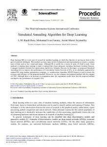
• at day nd of the present month, the following term is added to the objective function: nd −1 nd  nd   EHPi EHPi ∑ EHPj  ∑ ∑   j =1 i =1 ⋅ C PHP − PHPnd −1 =  in=1 − n −1 (14) nd  ⋅ C PHP d d  ∑ NHPi ∑ NHPj  NHPi ∑   i =1 j =1  i =1  In this case, the increase/reduction produced by the solution of day nd is divided by the first nd days of the present month. This procedure is justified by the fact that the cost of power consumption during peak hours is evaluated from the hourly average for the whole month. This optimization model is solved by a computer application (Figure 1) given by the connection between an optimizer, based on the Simulated Annealing method, and a hydraulic simulator, Sousa (2005).

Page 3064

Joint International Conference on Computing and Decision Making in Civil and Building Engineering June 14-16, 2006 - Montréal, Canada

problem results

problem data

Main Program

Optimizer - Simulated Annealing

iterations

Hydraulic behaviour

Candidate solution

(resolution of the optimization problem)

Hydraulic Simulator (hydraulic constraints)

Figure 1: Flowchart of the computer application developed to solve the optimal operation of water distribution systems problem. This tool functions as follows: throughout the search the optimizer generates candidate solutions (functioning of the controlling elements for each time period) and calls the hydraulic simulator to estimate the hydraulic behaviour of the system and evaluate the objective function. This cycle is repeated until the convergence criterion is met. The final result is the set of operating rules for the controlling elements that minimize the objective function value. Simultaneously, the application creates some additional files with information for analysing the behaviour of the Simulated Annealing method during the search, and files with detailed information about the final solution, namely: a file with the description of the energy costs calculation, a file with the reservoirs’ water level profiles and respective discharges, and a file with the hydraulic behaviour of the system at each simulated instant.

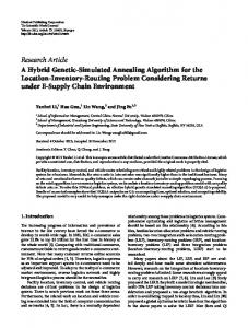
APPLICATIONS The applicability of the proposed methodology is illustrated with a hypothetical example of water distribution network (Figure 2). The complete data is available in Sousa (2005). This network is supplied by three fixed level reservoirs (FLR), each of which has a pump to increase the pressure in order to attain the minimum value imposed. To maintain adequate pressure levels during peak periods, the network has also three variable level reservoirs (VLR). This example leads to the resolution of a Mixed Integer Non Linear Programming problem with 72 binary decision variables and 1175 constraints. The first resolution was executed without considering either the power costs or the penalty term, to avoid too many pump functioning changes. The best solution obtained, after 6.5 minutes of execution time on a desktop computer Pentium IV 2.0MHz, presented an energy cost of €1249 (Figures 3 and 4), and a close observation of the results reveals some interesting aspects.

Page 3065

Joint International Conference on Computing and Decision Making in Civil and Building Engineering June 14-16, 2006 - Montréal, Canada

FLR - Fixed Level Reservoir VLR - Variable Level Reservoir VLR

Pump FLR

Pump

VLR

FLR

Pump FLR VLR

Figure 2: Scheme of the water distribution network. VLR 18

VLR 20

VLR 21

HRmin

HRmax

Reservoirs Water Level (m)

83 82 81 80 79 78 77 76 75 74 0 1 2 3 4 5 6 7 8 9 10 11 12 13 14 15 16 17 18 19 20 21 22 23 24

73

Time (h)

Figure 3: Solution with lowest energy cost – Reservoirs water levels. ( CE a = €1249; Nch = 11) The profiles of the variable water level reservoirs show five different phases, dictated by the daily variations in consumption and unit energy cost: almost complete filling up during the night to take advantage of the minimum energy cost; significant emptying as a result of the peak consumption and maximum energy cost; slight recovery during the early afternoon, taking profit of intermediate energy cost; almost complete emptying, due to peak

Page 3066

Joint International Conference on Computing and Decision Making in Civil and Building Engineering June 14-16, 2006 - Montréal, Canada

consumption and maximum energy cost; another slight recovery to achieve the minimum water level imposed at the end of the operating period, once again occurring during a low energy cost period. Another important point, since it contributes to water quality, is the fact that the daily operation involves the whole reservoir volume. With respect to pump functioning, avoiding having the pumps working during maximum energy cost periods (9.3012.00 and 18.30-21.00) is quite obvious. Besides this, it is quite intriguing why pump 31 only works for 2 hours throughout the entire operating period. This phenomenon is explained by the calculation of the pumps specific energy consumption: pump 29 - 0.339 kWh/m3; pump 30 - 0.356 kWh/m3; pump 31 - 0.404 kWh/m3. These values show clearly that, from the point of view of economy, pump 31 should only work in special situations, namely, when the functioning of the other two pumps is not satisfactory. Pump 29

Pump 30

Pump 31

Pumps discharge (l/s)

500 400 300 200 100

20-21 21-22 22-23 23-24

15-16 16-17 17-18 18-19 19-20

12-13 13-14 14-15

05-06 06-07 07-08 08-09 09-10 10-11 11-12

02-03 03-04 04-05

00-01 01-02

0

Time period (h) Figure 4: Solution with lower energy cost – Pumps discharges. ( CE a = €1249; Nch = 11) An attempt to reduce the number of pump functioning changes, Nch, was made by adding the term Pen to the objective function. The resolution of this newer version of the problem resulted in a solution with an energy cost of €1269, but with Nch=7 instead of the Nch=11 of Figure 3’s solution. This new solution implies a small increase in energy cost but simplifies the operation and increases pump motor lifetime. The same problem was again solved, but this time by considering variable speed pumps. For this scenario it was admitted that the pump speed, αr, could take seven different values, defined by αr=0, 0.5, 0.6, 0.7, 0.8, 0.9, 1.0 (αr=0 means that the pump is OFF and αr=1 means that the pump is working according to the initial characteristic curves). In this new optimization problem the decision variables are the pump speeds, defined by the αr values. The best solution found had an energy cost of €947 and implied 14 pump functioning changes (the introduction of the term Pen in the objective function led to a different solution with only 8 functioning changes, but with an energy cost of €964).

Page 3067

Joint International Conference on Computing and Decision Making in Civil and Building Engineering June 14-16, 2006 - Montréal, Canada

The comparison of these solutions’ costs (variable speed pumps) with those for the initial problem (fixed speed pumps) shows that, for this specific example, the introduction of the variable speed pumps reduced the energy cost by 24%, undoubtedly a considerable share of the total operating cost. This reduction in the energy cost is the consequence of a better adaptation of the variable speed pumps to the problem’s requirements, satisfying the conditions imposed with lower elevations, a fact that also resulted in lowering the maximum pressure values observed all over the network (a measure that can be viewed as a benefit in terms of water loss reduction). Now, suppose that the solution with an energy cost of €947 is to be implemented on day 15 of a certain month, the demanded power is 800 kW, and the power consumption during peak hours, calculated from the beginning of the month, is 400 kW. Assuming that CPC=1.230€/kW and CPHP=11.210€/kW, this would imply an increase in peak hours power consumption cost of €89, and an increase in demanded power cost of €116. However, as the increase in demanded power must be borne for the next 12 months, the global increase in power costs would be €1481 (89+12x116), making this apparently optimal solution a very bad planning decision. To avoid this mistake, the problem was solved considering the influence of the power cost. The best solution found was this: an energy cost of €976; a demanded power less than the maximum previously observed; an increase in the peak hours power consumption cost of €92; 14 pump functioning changes. The main advantage of this new solution is the fact that the cost increases only concern the present month, in contrast with the previous solution that implied a demanded power cost increase that had to be borne for 12 consecutive months, even if the power increase were not used anymore. This result is the consequence of the severe penalty imputed by the model to the increase in the demanded power. On the other hand, the penalty term Pen once again guided the search to solutions with small numbers of changes in pump functioning. Curiously, the resolution of this problem without that penalty led to quite a different solution: an energy cost equal to €964; no exceeding of the demanded power; an increase in the peak hours power consumption cost of €94; 34 pump functioning changes. To conclude, the slight cost reduction was achieved by the constantly changing pumps’ functioning. Recall that, besides helping to increase pump motor lifetime, this also creates a much more complex operation. This example is a good illustration of why the penalty applied to the changes in pump functioning was adopted.

CONCLUSIONS This paper presents a new approach to the optimal operation of water distribution systems problem. The methodology proposed here is based on optimization models that deal explicitly with the system’s hydraulic behaviour, and uses discrete variables to model pump functioning. This approach results in a Mixed Integer Non Linear Programming problem that is solved by the Simulated Annealing method. A hypothetical example of a water distribution network has been used to illustrate the methodology’s applicability and the outcome leads to the following conclusions: the operation rules obtained with the proposed methodology completely fulfil the conditions imposed and benefit from the daily variations in the unit energy cost; a slight increase in energy cost may allow a significant reduction in the number of pump functioning changes; for this example the use of variable speed pumps could produce significant reductions in the

Page 3068

Joint International Conference on Computing and Decision Making in Civil and Building Engineering June 14-16, 2006 - Montréal, Canada

energy cost; due to structure of the Portuguese energy tariff, it is extremely important to consider the power costs when defining operation rules. The results presented in this paper confirm that the use of this kind of tool could be of great help in defining operating rules for water supply systems, and even yield considerable benefits (economic and operational).

REFERENCES Brion, L.M., and Mays, L.W. (1991). “Methodology for optimal operation of pumping stations in water distribution systems.” J. of Hydraulic Engrg., ASCE, 117 (11) 15511569. de Schaetzen, W., Savic, D.A., and Walters, G.A. (1998). “A genetic algorithm approach to pump scheduling in water supply systems.” in Hydroinformatics 1998, Edited by V. Babovic, and L.C. Larsen, Balkema, Rotterdam, 897-899. Jowitt, P. W., and Germanopoulos, G. (1992). “Optimal pump scheduling in water-supply networks.” J. of Water Res. Planning and Mgmt., ASCE, 118 (4) 406-422. Lansey, K.E., and Awumah, K. (1994). “Optimal pump operations considering pump switches.” J. of Water Res. Planning and Mgmt., ASCE, 120 (1) 17-35. Nitivattananon, V., Sadowsky, E.C., and Quimpo, R.G. (1996). “Optimization of water supply system operation.” J. of Water Res. Planning and Mgmt., ASCE, 122 (5) 374-384. Ormsbee, L.E., and Reddy, S.L. (1995). “Nonlinear heuristic for pump operations.” J. of Water Res. Planning and Mgmt., ASCE, 121 (4) 302-309. Sousa, J.J.O. (2005). Decision Aid Models for the Design and the Operation of Water Supply Systems. Ph.D. Diss. (submitted), Civil Engrg., Univ. of Coimbra (in Portuguese). van Zyl, J.E., Savic, D.A., and Walters, G.A. (2004). “Operational optimization of water distribution systems using a hybrid genetic algorithm.” J. of Water Res. Planning and Mgmt., ASCE, 130 (2) 160-170. Yu, G., Powell, R.S., and Sterling, M.J.H. (1994). “Optimized pump scheduling in water distribution systems.” J. of Optimization Theory and Applications, 83 (3) 463-488. Zessler, U., and Shamir, U. (1989). “Optimal operation of water distribution systems.” J. of Water Res. Planning and Mgmt., ASCE, 115 (6) 735-752.

Page 3069