Hindawi Publishing Corporation Scientific Programming Volume 2016, Article ID 8048246, 14 pages http://dx.doi.org/10.1155/2016/8048246
Research Article Index Based Hidden Outlier Detection in Metric Space Honglong Xu,1,2,3 Rui Mao,1 Hao Liao,1 He Zhang,1 Minhua Lu,4 and Guoliang Chen1 1
Guangdong Province Key Laboratory of Popular High Performance Computers, College of Computer Science and Software Engineering, Shenzhen University, Shenzhen, Guangdong 518060, China 2 College of Information Engineering, Shenzhen University, Shenzhen, Guangdong 518060, China 3 School of Mathematics and Big Data, Foshan University, Foshan, Guangdong 528000, China 4 Guangdong Key Laboratory for Biomedical Measurements and Ultrasound Imaging, School of Biomedical Engineering, Shenzhen University, Shenzhen 518060, China Correspondence should be addressed to Minhua Lu;
[email protected] Received 30 November 2015; Revised 30 May 2016; Accepted 7 June 2016 Academic Editor: Michele Risi Copyright © 2016 Honglong Xu et al. This is an open access article distributed under the Creative Commons Attribution License, which permits unrestricted use, distribution, and reproduction in any medium, provided the original work is properly cited. Useless and noise information occupies large amount of big data, which increases our difficulty to extract worthy information. Therefore outlier detection attracts much attention recently, but if two points are far from other points but are relatively close to each other, they are less likely to be detected as outliers because of their adjacency to each other. In this situation, outliers are hidden by each other. In this paper, we propose a new perspective of hidden outlier. Experimental results show that it is more accurate than existing distance-based definitions of outliers. Accordingly, we exploit a candidate set based hidden outlier detection (HOD) algorithm. HOD algorithm achieves higher accuracy with comparable running time. Further, we develop an index based HOD (iHOD) algorithm to get higher detection speed.
1. Introduction In recent years, the rapid growth of multidimensional data brings about increasing demand for knowledge discovery, in which outlier detection is an important task with wide applications, such as credit card fraud detection [1], online video detection [2], and network intrusion detection [3]. As a matter of necessity, the wide use of outlier detection has aroused enthusiasm in many researchers. Over the past few decades, many outlier definitions and detection algorithms have been proposed in the literature [4–6]. Among these, statistics-based outlier detection [7, 8], which initiated a new era for data mining, has attracted an intensive study. Nevertheless, statistics-based outlier detection always depends on the probability distribution of the dataset, which is always priorly unknown. In order to overcome shortcoming of statistics-based method, Knorr and Ng et al. proposed distance-based definition and the corresponding detection method [9, 10]. According to his definition, an object O in a dataset T is
DB(𝑝, 𝐷) outlier if at least fraction p of the objects in T lies greater than distance D from O [10]. Soon afterwards, a number of distance-based definitions had been presented [4, 6]. Based on these definitions and their relevant detection methods, many researches significantly improved both outlier detection accuracy and speed. However, by existing definitions, outliers tend to be far from their nearest neighbors. As a result, if a small number of outliers are close to each other but are far from other points, which also known as outlier cluster, they are not likely to be determined as outliers because of their adjacency to each other. In this case, these points are hidden by each other. In other words, outlier itself has bad influence on detection accuracy [11]. In this paper, we propose a new perspective of hidden outlier that can uncover those hidden ones by traditional definitions and also design a new detection algorithm. Specifically, we make the following contributions: (1) A more accurate definition of outlier taking hidden outliers into consideration.
2
Scientific Programming (2) An effective detection algorithm for the definition proposed, with higher accuracy only at the cost of a little more time. (3) An index based HOD (iHOD) algorithm and getting much higher detection speed. (4) A simple but effective algorithm to select pivot for iHOD algorithm to avoid selecting outliers as pivots.
The rest of this paper is organized as follows. In Section 2, we will discuss several commonly used outlier definitions and relevant detection algorithms, along with their efficiency variants. Section 3 proposes the definition of hidden outlier and Section 4 proposes its detection algorithms. Experimental results are presented in Section 5, followed by conclusion and future work in Section 6.
2. Related Work As mentioned in the introduction, there are many definitions and detection algorithms for outliers, among which Hawkins’s work [12] stands out as the first. Following this work, three major distance-based definitions of outliers have been proposed, namely, k-R outlier [9, 10], k-distance-based outlier [13], and distance sum-based outlier [14]. k-R outlier [9, 10] in a dataset is a point that no more (𝑘,𝑅) than k points are within distance R to it, denoted as 𝑂thres [15]. Please note that the definition of k-R outlier is essentially equivalent to definition DB(𝑝, 𝐷) [9, 10], by which a point in a dataset T is an outlier if at least a fraction p of all points in T is beyond distance D to it. k-distance-based [13] outlier in a dataset is the point whose distance to its kth nearest neighbor is the largest among all points. Usually, the distance of a point to its kth nearest neighbor is considered as its outlier degree, and the n points with the largest outlier degrees are determined as (𝑘,𝑛) [15]. outliers, denoted as 𝑂𝑘max The definition of distance sum-based outlier [14] considered the sum of distances from a point to its k nearest neighbors as its outlier degree, and the n points with the largest sums are determined as outliers which can be denoted (𝑘,𝑛) . Similarly, distance average-based outlier, an equivas 𝑂𝑘sum alent definition in which the average distance to k nearest (𝑘,𝑛) neighbors is considered, can be defined and denoted as 𝑂𝑘avg [15]. Because kNN method is easy to implement [16], the above three distance-based definitions become popular. In addition, density-based outlier is actually distancebased outlier; for example, LOF [17], the most famous density-based definition, was accomplished in detecting outliers from a dataset with different densities, while ordinary definitions are not qualified for this work. Distance-based outlier detection algorithm was always designed for one or several definitions. Over the past decades, many detection algorithms were proposed since the above definitions emerged, in which the most famous one is ORCA [18]. ORCA has been honoured as the state-of-art algorithm [18] because of its simplicity and efficiency. What is more, it supports any outlier definitions with monotonically decreasing function of the nearest neighbor distances such
(𝑘,𝑛) (𝑘,𝑛) or 𝑂𝑘avg . After that, many variants appeared in the as 𝑂𝑘max literature, including solving set algorithm [19], MIRO [20], RCS [21], and iORCA [22]. It should be noted that not all the variants support the same definitions as ORCA [18]; for (𝑘,𝑛) definition. instance, iORCA [22] could not support 𝑂𝑘avg For speeding up kNN search [16], some researchers exploit other research methods, for example, index based algorithm. Knorr et al. first bring forward index based method. According to their description, R-tree and k-d tree can be applied [10]. After that, k-d tree based method was proposed and had got a time complexity of 𝑂(𝑛𝑘) [23]. Other detection algorithms, including HilOut based algorithm [24], P tree based algorithm [25], LSH based algorithm [26, 27], and SFC index [28], use different index structure to speed up detection. Besides, sample method was applied to reduce distance computations [29]. k-R outlier also attracted many researchers since Knorr and Ng et al. proposed DB(𝑝, 𝐷) outlier definition and three relevant algorithms (nested-loop, index based, and cell-based algorithm) [9, 10]. For example, Tao et al.’s SNIF algorithm [30] can detect all outliers by scanning the dataset at most twice and even once in some cases. DOLPHIN algorithm [31] is also an efficient method to detect k-R outlier. However, k-R outlier has a shortcoming that parameters are difficult to set [13]. Similarly, the research works for density-based detection algorithm started from their incipient definition, which is LOF [17]. The variants or improved algorithms included COF [32], MDEF [33], Ensemble method [34], and so forth. Since this paper aimed at outlier definition, we just took three most popular and simplest algorithms as comparison algorithm: ORCA [18], which is the state-of–art distancebased outlier detection algorithm, LOF [17], the most representative density-based outlier detection method, and iORCA [22], latest index based outlier detection algorithm in (𝑘,𝑛) (𝑘,𝑛) and 𝑂𝑘max were metric space. For ORCA and iORCA, 𝑂𝑘sum used as outlier definition, respectively.
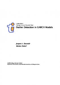
3. Definition of Hidden Outlier In this section, we propose the new perspective of hidden outlier. The basic idea is that once an outlier is detected, exclude it from the nearest neighbors of other points. 3.1. Cause of Hidden Outlier. As is shown in Figure 1, points A and B are outliers, but point C is not. In this case, if we set 𝑘 = 2 and detect TOP 2 outliers by distance sum-based outlier definition, A and C will be detected as outliers, other than B, which is a real outlier. However, A and C will be detected as outliers, other than B, which is a real outlier. The reason is that the existence of A reduces the outlier degree of B, leading to the mistake in detection. 3.2. Definition of Hidden Outlier. If a small number (e.g., equal to or greater than 2) of points are close to each other but are far to other points, they are usually deemed as outliers. However, traditional distance-based definitions of outliers determine an outlier by its distances to its nearest neighbors.
Scientific Programming
3
As a result, those small number of points close to each other are usually not outliers according to traditional definitions. In this situation, outliers seem to be hidden by each other, and they can be called hidden outliers. Our definition of outliers which include hidden ones, denoted as 𝐻𝑂(𝑘,𝑛) 𝑘sum , is extended from the definition of distance-based outlier. Here we take distance sum-based out(𝑘,𝑛) , as example to give detailed description. Notation lier, 𝑂𝑘sum summarizes the notations and their description. Let D be a dataset, let dist be a distance function, let p be a point, and let 𝑛𝑛𝑖 (𝑝, 𝐷) be the ith nearest neighbor of p in D. Please note that a point is not considered as a nearest (𝑘,𝑛) neighbor of itself. Further, let 𝐷𝑖,𝑘 be the ith outlier by 𝑂𝑘sum definition, let 𝑤𝑘 (𝑝, 𝐷) be the outlier degree of 𝑝, and let 𝐷𝑛 outlier be the set of 𝑛 outliers of the largest values of outlier (𝑘,𝑛) , 𝑤𝑘 (𝑝, 𝐷) is given degree. According to the definition of 𝑂𝑘sum by
5
4 A (4, 4) 3 C (0, 3)
B (4, 3)
2
1
0 0
1
2
3
4
5
6
Figure 1: A simple 2-dimension dataset.
𝑘
𝑤𝑘 (𝑝, 𝐷) = ∑dist (𝑝, 𝑛𝑛𝑖 (𝑝, 𝐷)) .
(1)
𝑖=1
Let 𝐻𝐷𝑖,𝑘 be the ith outlier by our new definition, let 𝐻𝑤𝑘 (𝑝, 𝐷) be p’s outlier degree, and let 𝐻𝐷𝑛 -outlier be the set of first n outliers. Definition 1. The definition of outliers include hidden ones, 𝐻𝑂(𝑘,𝑛) 𝑘sum , defines the outliers in an iterative way: 𝐻𝐷1,𝑘 = argmax𝑝 (𝑤𝑘 (𝑝, 𝐷)) 𝐻𝐷𝑖,𝑘 = argmax𝑝 (𝑤𝑘 (𝑝, 𝐷 − 𝐻𝐷𝑖−1 -outlier)) ,
(2)
2 ≤ 𝑖 ≤ 𝑛. Definition 2. The outlier degree of p by 𝐻𝑂(𝑘,𝑛) 𝑘sum definition, 𝐻𝑤𝑘 (𝑝, 𝐷), is defined as 𝐻𝑤𝑘 (𝑝, 𝐷) if 𝑝 = 𝐷1,𝑘 𝑤𝑘 (𝐷1,𝑘 , 𝐷) , { { { { = {𝑤𝑘 (𝑝, 𝐷 − 𝐻𝐷𝑖−1 -outlier) , if 𝑝 = 𝐻𝐷𝑖,𝑘 , 2 ≤ 𝑖 ≤ 𝑛 { { { otherwise. {𝑤𝑘 (𝑝, 𝐷 − 𝐻𝐷𝑛 -outlier) ,
(3)
In other words, 𝐻𝑤𝑘 (𝑝, 𝐷) is still the sum of distances from p to its k nearest neighbors, while outliers already detected are not considered as p’s nearest neighbors. Please note that the sequence of 𝐻𝑤𝑘 (𝐻𝐷𝑖,𝑘 , 𝐷), 1 ≤ 𝑖 ≤ 𝑛, might not be in descending order. The other definition of outliers may be deduced by (𝑘,𝑛) , we can simply displace the analogy. For example, 𝑂𝑘max (𝑘,𝑛) (𝑘,𝑛) outlier degree of 𝑂𝑘sum as that of 𝑂𝑘max , which is 𝑤𝑘 (𝑝, 𝐷) = dist (𝑝, 𝑛𝑛𝑖 (𝑝, 𝐷)) .
(4)
Then we can give the same definition of hidden outlier and its degree as Definitions 1 and 2. It is worth mentioning (𝑘,𝑛) based hidden outlier will be called that, for simplicity, 𝑂𝑘sum (𝑘,𝑛) ksum hidden outlier, while 𝑂𝑘max hidden outlier will be called
kmax hidden outlier. Though both HOD (Section 4.1) and iHOD (Section 4.2) can apply these two definitions, for the limited space, they will only use one definition, respectively, in our experiments.
4. Hidden Outlier Detection Algorithm In this section, the detection algorithms designed for hidden outlier are proposed, together with several theorems and definitions. 4.1. Hidden Outlier Detection Algorithm. The detection algorithm of 𝐻𝑂(𝑘,𝑛) 𝑘sum is presented in this section. We start from a few theorems and concepts together which can be used to speed up the detection. Theorem 3. The hidden outlier degree is always no less than the outlier degree or 𝐻𝑤𝑘 (𝑝, 𝐷) ≥ 𝑤𝑘 (𝑝, 𝐷). The proof is straightforward from the definitions of both outlier degrees and is thus omitted. Theorem 4. The ith hidden outlier’s outlier degree is no less (𝑘,𝑛) than that of the ith outlier by 𝑂𝑘𝑠𝑢𝑚 ; that is, 𝐻𝑤𝑘 (𝐻𝐷𝑖,𝑘 , 𝐷) ≥ 𝑤𝑘 (𝐷𝑖,𝑘 , 𝐷), 1 ≤ 𝑖 ≤ 𝑛. Proof. (1) if 𝑖 = 1, the equation clearly holds. (2) If 2 ≤ 𝑖 ≤ 𝑛, one has the following. (a) If 𝐻𝐷𝑖 -outlier = 𝐷𝑖 -outlier, there must exist t, such that 𝐻𝐷𝑖,𝑘 = 𝐷𝑡,𝑘 , 1 ≤ 𝑡 ≤ 𝑖. From Theorem 3 and the definition of 𝑤𝑘 (𝑝, 𝐷), 𝐻𝑤𝑘 (𝐻𝐷𝑖,𝑘 , 𝐷) ≥ 𝑤𝑘 (𝐷𝑡,𝑘 , 𝐷) ≥ 𝑤𝑘 (𝐷𝑖,𝑘 , 𝐷) .
(5)
(b) Otherwise, there must exist t, such that 𝐷𝑡,𝑘 ∉ 𝐻𝐷𝑖 outlier, 1 ≤ 𝑡 ≤ 𝑖. From Definition 2, Theorem 3, and the definition of 𝑤𝑘 (𝑝, 𝐷), 𝐻𝑤𝑘 (𝐻𝐷𝑖,𝑘 , 𝐷) ≥ 𝐻𝑤𝑘 (𝐷𝑡,𝑘 , 𝐷) ≥ 𝑤𝑘 (𝐷𝑡,𝑘 , 𝐷) ≥ 𝑤𝑘 (𝐷𝑖,𝑘 , 𝐷) .
(6)
4
Scientific Programming
Input: 𝑘, 𝑛, 𝐷 Output: 𝐻𝐷𝑛 -outlier (1) 𝑐 ← 0; (2) 𝐷𝑛 -𝑜𝑢𝑡𝑙𝑖𝑒𝑟 ← 𝜙; (3) 𝐵 ← 𝜙; //𝐵 is a data block of dataset 𝐷 (4) while 𝐵 ← get-next-block(𝐷) { (5) for each 𝑑 in 𝐷 { (6) for each 𝑏 in 𝐵 { (7) 𝑑𝑖𝑠 ← dist(𝑏, 𝑑); update 𝑏.NN (8) if 𝑀𝑃𝑊𝑛,𝑘 (𝑏, 𝐷) < 𝑐 remove 𝑏 from 𝐵; }} (9) for each 𝑏 in 𝐵 { (10) 𝐷𝑛 -𝑜𝑢𝑡𝑙𝑖𝑒𝑟 ← TOP(𝐵 ∪ 𝐷𝑛 -𝑜𝑢𝑡𝑙𝑖𝑒𝑟, 𝑛) //update 𝐷𝑛 -𝑜𝑢𝑡𝑙𝑖𝑒𝑟; //update 𝑐; (11) 𝑐 ← 𝑤𝑘 (𝐷𝑛,𝑘 , 𝐷) (12) for each cs in 𝐶𝑆𝑛,𝑘 (𝐷) { (13) if (𝑀𝑃𝑊𝑛,𝑘 (𝑐𝑠, 𝐷) < 𝑐) (14) delete cs from 𝐶𝑆𝑛,𝑘 (𝐷); } (15) if (𝑀𝑃𝑊𝑛,𝑘 (𝑏, 𝐷) > 𝑐) (16) insert 𝑏 to 𝐶𝑆𝑛,𝑘 (𝐷); }} (17) 𝐻𝐷𝑛 -𝑜𝑢𝑡𝑙𝑖𝑒𝑟 ← filtering process(𝐷𝑛 -𝑜𝑢𝑡𝑙𝑖𝑒𝑟, 𝐶𝑆𝑛,𝑘 (𝐷)); (18) return 𝐻𝐷𝑛 -𝑜𝑢𝑡𝑙𝑖𝑒𝑟; Algorithm 1: Hidden outlier detection algorithm.
For convenience, we introduce two more definitions, maximum possible outlier degree and hidden outlier candidate set, and related theorems to show their properties. Definition 5. The maximum possible outlier degree of p, 𝑀𝑃𝑊𝑛,𝑘 (𝑝, 𝐷), is the hidden outlier degree of p assuming that all the first 𝑛 − 1 nearest neighbors of p are detected as outliers and thus are excluded from contributing to p’s hidden outlier degree. That is, 𝑛+𝑘−1
𝑀𝑃𝑊𝑛,𝑘 (𝑝, 𝐷) = ∑ dist (𝑝, 𝑛𝑛𝑖 (𝑝, 𝐷)) .
(7)
𝑖=𝑛
From Definition 5, we give the following obvious theorem without proof. Theorem 6. 𝐻𝑤𝑘 (𝑝, 𝐷) ≤ 𝑀𝑃𝑊𝑛,𝑘 (𝑝, 𝐷) .
(8)
Definition 7. The hidden outlier candidate set, 𝐶𝑆𝑛,𝑘 (D), is a subset of D such that, for each 𝑝 ∈ 𝐶𝑆𝑛,𝑘 (𝐷), 𝑀𝑃𝑊𝑛,𝑘 (𝑝, 𝐷) ≥ 𝑤𝑘 (𝐷𝑛,𝑘 , 𝐷). The following theorem shows the purpose in defining hidden outlier candidate set. Theorem 8. The hidden outlier candidate sets, 𝐶𝑆𝑛,𝑘 (D), contains all of the outliers defined by 𝐻𝑂(𝑘,𝑛) 𝑘𝑠𝑢𝑚 . Proof. For an arbitrary outlier p defined by 𝐻𝑂(𝑘,𝑛) 𝑘sum , from definition and from Theorem 4, 𝐻𝑤𝑘 (𝑝, 𝐷) ≥ 𝑤𝑘 (𝑝, 𝐷). From Theorem 6, H𝑤𝑘 (𝑝, 𝐷) ≤ 𝑀𝑃𝑊𝑛,𝑘 (𝑝, 𝐷). As a result, 𝑀𝑃𝑊𝑛,𝑘 (𝑝, 𝐷) ≥ 𝑤𝑘 (𝐷𝑛,𝑘 , 𝐷); that is, 𝑝 ∈ 𝐶𝑆𝑛,𝑘 (𝐷).
Our hidden outlier detection (HOD) algorithm (Algorithm 1) is based on the ORCA algorithm [18]. HOD searches 𝑘 + 𝑛 − 1 nearest neighbors (in consideration of performance, n must be small) of every data block (lines (4)–(7)). Once an object is impossible to become an outlier, it will be removed from data block (line (8)). After processing a data block, HOD gets current 𝐷𝑛 -outlier (line (10)) and updates cutoff value c (line (11)) and then maintains hidden outlier candidate set at the same time (lines (12)–(16)), including deleting the objects with smaller MPW than c (lines (13)-(14)) and adding the objects with larger MPW than c (lines (15)-(16)). Finally the candidate set is filtered to get the final results (Algorithm 2). Algorithm 2 shows how the candidate set is filtered to get the final results. 𝐷1,𝑘 is first moved from 𝐶𝑆𝑛,𝑘 (D) to 𝐻𝐷𝑛 -outlier (line (1)), because the first outlier of 𝐷𝑛 -outlier and first outlier 𝐻𝐷𝑛 -outlier are the same. Then the last outlier of 𝐻𝐷𝑛 -outlier is checked to see whether it is a nearest neighbor of some objects in 𝐶𝑆𝑛,𝑘 (D). If yes, it is deleted from that object’ nearest neighbors and the hidden outlier degree 𝐻𝑤𝑘 (𝑐𝑠𝑜, 𝐷) (lines (2)–(4)) is updated. Next, the object with the largest hidden outlier degree in 𝐶𝑆𝑛,𝑘 (D) is moved to 𝐻𝐷𝑛 -outlier (line (5)), and the process goes back to line (2) until there are n outliers (line (6)). As Bay and Schwabacher indicated, ORCA [18] has 𝑂(𝑁) time complexity on average and 𝑂(𝑁2 ) in the worst case. In contrast to ORCA [18], HOD searches more nearest neighbors and thus costs more time and memory space. Further, HOD prunes less normal objects and results in more distance computations. However, these do not increase HOD’s time complexity because as more data blocks have been processed, the cutoff value c becomes larger and more normal objects will be pruned. In other words, the pruning mechanism is the same as ORCA [18]. After searching a data block’s nearest neighbors, HOD maintains an outlier candidate set
Scientific Programming
5
Input: 𝐷𝑛 -𝑜𝑢𝑡𝑙𝑖𝑒𝑟, 𝐶𝑆𝑛,𝑘 (𝐷) Output: 𝐻𝐷𝑛 -𝑜𝑢𝑡𝑙𝑖𝑒𝑟 (1) 𝐻𝐷1,𝑘 = 𝐷1,𝑘 , delete 𝐷1,𝑘 from 𝐶𝑆𝑛,𝑘 (𝐷); (2) Set 𝑖 = 1; (3) for each cso in 𝐶𝑆𝑛,𝑘 (𝐷) { (4) if (𝐻𝐷𝑖,𝑘 ∈ 𝑐𝑠𝑜.𝑁𝑁) update cso.NN and 𝐻𝑤𝑘 (𝑐𝑠𝑜, 𝐷); } (5) 𝑖++; 𝐻𝐷𝑖,𝑘 ← TOP(𝐶𝑆𝑛,𝑘 (𝐷), 1), delete it from 𝐶𝑆𝑛,𝑘 (𝐷) and insert to 𝐻𝐷𝑛 -outlier; (6) if (𝑖 < 𝑛) do line (3) (7) return 𝐻𝐷𝑛 -outlier; Algorithm 2: Filtering process.
Input: 𝐷, pivot Output: index 𝐿 (1) 𝐿 ← 𝜙; (2) for each 𝑜 in 𝐷 (3) 𝐿(𝑜) ← dist(𝑝𝑖V𝑜𝑡, 𝑜); (4) sort(𝐿); //sorted by the distance value in //descending order (5) return 𝐿; Algorithm 3: Build index.
and updates it after updating c, which can be implemented by a fast priority queue. In addition, experimental results show that the candidate set size keeps constant as a whole with various dataset sizes, limiting the overhead of filtering process described in Algorithm 2. 4.2. Index Based Hidden Outlier Detection Algorithm. In order to speed up HOD algorithm, we draw on the experience of iORCA and develop a simple index based hidden outlier detection algorithm. As we discussed in Section 2, iORCA is a very excellent distance-based improvement from ORCA, which is the state-of-the-art method in outlier detection. It is worth mentioning that the build index process (Algorithm 3) of iORCA is very simple and almost costs little time. However, the only fly in the ointment is that iORCA is short of pivot selection method. Addressing this shortcoming, we propose a simple but efficient pivot selection algorithm (Algorithm 4). The most important idea of iORCA is to update the cutoff value faster. In Algorithm 3, we can see that, in order to achieve this goal, iORCA simply calculates the distance between every object to pivot (lines (2)-(3)) and then sort them from large to small (line (4)). Obviously, both the time and memory consuming of this index are very small. The largest difference between similarity search and outlier detection is that similarity search procedure may be used many times, for searching different object, while outlier detection procedure may be used for only several times, even just one time. That is a decision that their pivot selection method for building index will be different. Since similarity search always follows the rules of Offline Construction and Online Search [35, 36], it can spend more time to select pivots
Input dataset
Pivot selection in a small set of dataset
Build index for the whole dataset
Output hidden outlier
Filter hidden outlier
Build hidden outlier candidate set
Figure 2: The flow chart of iHOD algorithm.
and build index, other than outlier detection to save time in this stage. As Bhaduri et al. said that if we select inlier points as pivots, the points farthest from them will be more likely to be the outliers [22]. To benefit from this, the goal of our pivot selection algorithm is to select density points as pivots. However, the accurate search of density points is too expensive. So, in our pivot selection algorithm, we only find out the approximate density regions (lines (4)-(5)) and then choose the middle point of these regions (line (6)). In addition, we only take a part of dataset to select pivots, and usually a data block is enough. Due to the small percentage of outliers, it is almost impossible to select outliers as pivots via this subset using our method. The flowchart of iHOD algorithm is shown in Figure 2. The stopping rule (Theorem 9) of iORCA can be applied in iHOD as well to quickly stop updating the cutoff value. Theorem 9 (iORCA stopping rule [22]). Let 𝐷 be the dataset, let 𝑐 be the cutoff value, let 𝑝 be the pivot, and let 𝑥𝑡 be any test point currently being tested by iORCA (or iHOD); if dist (𝑥𝑡 , 𝑝) + dist (𝑝, 𝑛𝑛𝑘 (𝑝, 𝐷)) < 𝑐
(9)
then iORCA (or iHOD) can terminate with the correct 𝐷𝑛 outlier and cutoff value. In addition, we propose other rules to reduce the distance computing times. Theorem 10. If dist(𝑥𝑡 , 𝑝) + dist(𝑝, 𝑛𝑛𝑘+𝑛−1 (𝑝, 𝐷)) < 𝑐, then iHOD can stop updating hidden outlier candidate set. Theorem 10 can be proved similar to Theorem 9.
6
Scientific Programming
Input: 𝐷, 𝑝𝑖V𝑜𝑡𝑁𝑢𝑚 Output: 𝑝𝑖V𝑜𝑡 (1) blockIndex ← 𝜙; (2) 𝐵 ← getPartOfDataSet(𝐷); //𝐵 is usually a data block of dataset 𝐷 (3) blockIndex ← buildIndex(𝐵, 𝐵[0]); (4) divide blockIndex into partNum equal segments; //𝑝𝑎𝑟𝑡𝑁𝑢𝑚 ⩾ 2 ∗ 𝑝𝑖V𝑜𝑡𝑁𝑢𝑚 and 10, every segment has the same number of points (5) get pivotNum segments with smallest skip distance; (6) pivot ← middle object of every smallest segment; (7) return pivot; Algorithm 4: Pivot selection.
Input: 𝑘, 𝑛, 𝐷 Output: 𝐻𝐷𝑛 -𝑜𝑢𝑡𝑙𝑖𝑒𝑟 (1) 𝑐 ← 0; 𝐷𝑛 -𝑜𝑢𝑡𝑙𝑖𝑒𝑟 ← 𝜙; 𝐵 ← 𝜙; //𝐵 is a data block of dataset 𝐷 (2) pivot ← pivotSelection(𝐷, 1); (3) 𝐿 ← buildIndex(𝐷, pivot); //𝐿 is a data block of dataset 𝐷 (4) while 𝐵 ← get-next-block(𝐿(𝐷)){ (5) if (Theorem 10 holds for 𝐵(1)) then break; (6) else { (7) 𝜇 ← findAvg(𝐿(𝐵)); (8) 𝑠𝑡𝑎𝑟𝑡𝐼𝐷 ← find(𝐿 ⩾ 𝜇); (9) 𝑜𝑟𝑑𝑒𝑟 ← spiralOrder(L.id, startID); (10) for each 𝑑 in 𝐷 with order { (11) for each 𝑏 in 𝐵 { (12) if (Theorem 11 doesn’t hold for 𝑑 and 𝑏) { (13) 𝑑𝑖𝑠 ← dist(𝑏, 𝑑); update 𝑏.NN (14) if 𝑀𝑃𝑊𝑛,𝑘 (𝑏, 𝐷) < 𝑐 remove 𝑏 from 𝐵; }}} (15) for each 𝑏 in 𝐵 { (16) if (Theorem 9 doesn’t holds for 𝐵(1)) { //update 𝐷𝑛 -𝑜𝑢𝑡𝑙𝑖𝑒𝑟; (17) 𝐷𝑛 -𝑜𝑢𝑡𝑙𝑖𝑒𝑟 ← TOP(𝐵 ∪ 𝐷𝑛 -𝑜𝑢𝑡𝑙𝑖𝑒𝑟, 𝑛) (18) 𝑐 ← 𝑤𝑘 (𝐷𝑛,𝑘 , 𝐷) //update 𝑐; (19) for each cs in 𝐶𝑆𝑛,𝑘 (𝐷) { (20) if (𝑀𝑃𝑊𝑛,𝑘 (𝑐𝑠, 𝐷) < 𝑐) (21) delete cs from 𝐶𝑆𝑛,𝑘 (𝐷); } (22) if (𝑀𝑃𝑊𝑛,𝑘 (𝑏, 𝐷) > 𝑐) (23) insert 𝑏 to 𝐶𝑆𝑛 , 𝑘(𝐷); }}} (24) 𝐻𝐷𝑛 -𝑜𝑢𝑡𝑙𝑖𝑒𝑟 ← filtering process(𝐷𝑛 -𝑜𝑢𝑡𝑙𝑖𝑒𝑟, 𝐶𝑆𝑛,𝑘 (𝐷)); (25) return 𝐻𝐷𝑛 -𝑜𝑢𝑡𝑙𝑖𝑒𝑟; Algorithm 5: Index based hidden outlier detection algorithm.
Theorem 11. If dist (𝑥𝑖 , 𝑝) − dist (𝑥𝑗 , 𝑝) > dist (𝑥𝑖 , 𝑛𝑛𝑘 (𝑥𝑖 , 𝐷))
(10)
then 𝑥𝑖 is no longer the k nearest neighbors of 𝑥𝑖 . Proof. Using Triangle Inequality, there is dist (𝑥𝑖 , 𝑥𝑗 ) ≥ dist (𝑥𝑖 , 𝑝) − dist (𝑥𝑗 , 𝑝)
Our index based hidden outlier detection algorithm (Algorithm 5) combines iORCA (lines (3)–(9)) and HOD (lines (13)–(24)) algorithms and updates them with pivot selection algorithm (line (2)) and Theorem 11 (line (12)), finally resulting in its high performance.
5. Experimental Results (11)
(12)
In this section, we compare HOD and iHOD algorithm with ORCA [18], iORCA [22], and LOF [17], three popular distance-based outlier detection algorithms, in both accuracy and efficiency.
In other words, 𝑥𝑗 is faster than the 𝑘th nearest neighbor of 𝑥𝑖 . So 𝑥𝑗 is no longer the 𝑘 nearest neighbors of 𝑥𝑖 .
5.1. Test Suite. We follow a common way [37] in constructing the test suite. Four popular real world classification datasets
so we have dist (𝑥𝑖 , 𝑥𝑗 ) > dist (𝑥𝑖 , 𝑛𝑛𝑘 (𝑥𝑖 , 𝐷)) .
Scientific Programming are picked from the UCI Machine Learning Repository [38], and then a few objects from a class of small cardinality together with other larger classes are finally picked as the test suite. The first dataset is from the KDD Cup 1999 dataset, used by Yang [37]. The first 20,000 TCP data of its ten percent version, which has 76 abnormal connections or outliers, are picked. The second dataset is from the Optdigits (short for Optical Recognition of Handwritten Digits) dataset. The first 10 records from class 0, served as outliers, together with other 3,447 records are picked. The third one is from the Breast Cancer Wisconsin (Diagnostic) dataset. The first 10 records of the malignant ones, served as outliers, are picked, making 367 as the total number of records. The last one is from the Heart Disease dataset. All records in class 4, serving as outliers, together with other records except in classes 1–3 are picked. Altogether, there are 203 records with 15 outliers in dataset 4. After a simple constructing, these four datasets are match for Hawkins’s outlier definition [12], which is generally acceptable. 5.2. Evaluation Methodology. In statistics, a receiver operating characteristic (ROC) or ROC curve is a graphical plot that illustrates the performance of a binary classifier system as its discrimination threshold is varied. The curve is created by plotting the true positive rate (TPR) against the false positive rate (FPR) at various threshold settings. Calculate the Area Under Curve (AUC), and the larger it is, the better it is. With regard to outlier detection, as mentioned before, let D be the dataset, let |D| be the dataset size, and let n be the various threshold setting parameter. In other words, when n is set as a specific value, the top-n outliers will be identified as outliers, and other |𝐷|−𝑛 points in the dataset are regarded as inliers. So, for a specific n, we can get a couple value of TPR and FPR. Vary n from 0 to |D|; we can easily get the ROC curve and then calculate the AUC value. Obviously, the above calculation is in the case that neighbor number k is specific. If we vary it, then we can get the AUC-k graphical plot, which make us easily see the outlier detection accuracy with regard to parameter k. 5.3. Experimental Results. The experiments were run on a desktop with Intel Core 3.40 GHz processor, 8 GB RAM, running Windows 7 Professional Service Pack 1. The algorithms were implemented in C++ and compiled with Visual Studio 2012 in Release Mode. Unless otherwise specified, both the parameters k in determining nearest neighbors and detecting outlier number n are set as 10. The accuracy is first studied, then the running time and performance of pivot selection algorithm at last. 5.3.1. Accuracy. The accuracy of the five algorithms, namely, HOD, ORCA [18], iHOD, iORCA [22], and LOF [17], is first studied by way of AUC. For each constant value of k, the AUC values of the three algorithms with various values of n are computed. Then the AUC values of various values of (𝑘,𝑛) k are plotted in Figure 3. Please note that ORCA uses 𝑂𝑘sum definition, and HOD uses its extensional ksum hidden outlier, (𝑘,𝑛) definition, and iHOD uses kmax while iORCA uses 𝑂𝑘max hidden outlier.
7 Table 1: Rankings obtained through Friedman’s test over average true positives of Figure 4. Algorithm Ranking
ORCA 3.75
HOD 3.25
LOF 5
iORCA 1.875
iHOD 1.125
It can be seen that HOD and ORCA achieve higher AUC values than LOF for almost all of the cases, for the four datasets. Further, HOD is better than ORCA for most of the cases. For the cases when ORCA is better than HOD, the values are close to 1, and the difference is thus marginal. Also, we can see the appearance of iHOD and iORCA. To see the difference more clearly, we further compare the three algorithms by way of true positives (Figure 4). Obviously, iHOD is the best in most cases while LOF is the worst for almost all of the cases. Particularly, the true positives of LOF are close to 0 for the KDD Cup 1999 and Optdigits dataset. In Figure 4(c), we can see that HOD and iHOD have got the true positives similar to ORCA and iORCA, respectively. This is because Breast Cancer Wisconsin (Diagnostic) dataset is free of outliers hidden by other ones. In order to see more details about the performance of iHOD, we also do some Non-Parametric Tests [39], including Friedman’s test [40] and Hochberg’s procedure [41]. However, even though Hochberg’s testing results show that the difference between iHOD and iORCA is insignificant, it can be seen from Figures 3 and 4 that iHOD has actually made improvements from iORCA, which is an excellent outlier detection algorithm. Table 1, which is the rankings of average true positives from Figure 4, also shows that iHOD outperforms iORCA. 5.3.2. Efficiency. As mentioned earlier, an extra piece of work of HOD and iHOD is to filter through the candidate set, which may cost much time if the candidate set size is too large. The candidate size with respect to values of n (Figure 5) and dataset size (Figure 6) are plotted. The Breast Cancer Wisconsin (Diagnostic) dataset and the Heart Disease dataset are not included due to their tiny sizes. Clearly, the candidate set size is not strongly correlated to the dataset size, making its effect to the running time limited. The running time of the seven algorithms for the KDD Cup 1999 dataset and the Optdigits dataset is listed in Figure 7, respectively. Please note that HOD has better accuracy than ORCA [18] and LOF [17], while iHOD is better than almost all algorithms, as indicated in last section. To make the comparison fair, we extend ORCA and iORCA [22] to HORCA and HiORCA to achieve the same detection results of HOD and iHOD. That is, run ORCA or iORCA n times, while each time only one outlier is detected and is removed from following runs. The running time of HORCA and HiORCA is also listed in the tables. The figure shows clearly that the running time of LOF increases dramatically as the dataset size increases. HOD, with better accuracy, takes almost 1.5 times of the time as that of ORCA [18]. However, HORCA, with the equivalent accuracy as that of HOD, takes up to 9 times of the running time as that of HOD. To our surprise, iHOD runs even faster
8
Scientific Programming 1 0.9
0.8
AUC
AUC
0.7
0.6 0.5
0.4
0.3 0
50
150
100
200
250
0
20
k
iHOD LOF
ORCA iORCA HOD
40 k
iHOD LOF
ORCA iORCA HOD
(a) KDD Cup 1999
(b) Optdigits
1 0.9 0.9
0.8 AUC
AUC
0.7
0.7
0.5 0.6
0.3
0.5 0
20
40
0
20
ORCA iORCA HOD
40 k
k
iHOD LOF
(c) Breast Cancer Wisconsin (Diagnostic)
ORCA iORCA HOD
iHOD LOF (d) Heart Disease Dataset
Figure 3: AUC values with various values k of five algorithms for four datasets.
than iORCA [22]. This is because iHOD uses Theorem 10 to get a large reduction of distance calculation times. 5.3.3. Performance of Pivot Selection Algorithm. In order to estimate the performance of pivot selection algorithm, we compare iORCA/iHOD with/without pivot selection algorithm, in both running time and distance calculation times. For the sake of accuracy, we ran every experiment setup for 10 times and then get their standard deviation and mean value. From Tables 2 and 3, we can see that our pivot selection algorithm makes the experiment results very stable and even
gets better results in mean value of running time and distance calculation times. As other popular outlier detection algorithms like ORCA [18], iORCA [22], and LOF [17], both HOD and iHOD have two parameters, which are nearest neighbor number k and outlier number n. However, for these two parameters, it is unwise to decrease their value in order to get improvement in efficiency, because it may seriously reduce the detection (𝑘,𝑛) an so on. Though n quality. In fact, k can be set refer to 𝑂𝑘avg is in proportion to candidate set size, thereby increasing the running time. Fortunately, n depends on user’s requirement, so it is usually not large.
Scientific Programming
9
35
12
30
10
25 True positive
True positive
8 20 15
6 4
10
2
5 0
0 20
40
60 n
80
100
10
iORCA iHOD
ORCA HOD LOF
20
30 n
40
50
80
100
iORCA iHOD
ORCA HOD LOF
(a) KDD Cup 1999
(b) Optdigits
16
12
14
10
12 True positive
True positive
8 6 4
10 8 6 4
2
2
0
0 10
20
30 n
40
50
40
60 n
iORCA iHOD
ORCA HOD LOF
20
iORCA iHOD
ORCA HOD LOF
(c) Breast Cancer Wisconsin (Diagnostic)
(d) Heart Disease Dataset
Figure 4: True positive values with various values n of five algorithms for four datasets.
Table 2: Standard deviation and mean value of running time (milliseconds) over KDD Cup 1999 dataset. Size Category iORCA random iORCA psm iHOD random iHOD psm
5,000 Standard deviation
Mean value
16.7 4.9 39.0 21.2
697.60 688.10 216.70 232.20
10,000 Standard Mean value deviation 1,363.50 8.0 1,379.10 8.1 368.10 96.4 309.00 35.9
15,000 Standard Mean value deviation 2,040.60 21.7 2,098.20 34.6 405.60 54.6 402.60 83.2
20,000 Standard Mean value deviation 2,725.40 78.5 2,717.60 26.1 458.80 33.6 441.60 22.2
Scientific Programming
14
14
12
12
10
10
Candidate set size (×102 )
Candidate set size (×102 )
10
8 6 4 2
8 6 4 2
0
0 0
50
100
150
200
0
10
20
n
30
40
50
n
HOD iHOD
HOD iHOD (a) KDD Cup 1999
(b) Optdigits
Figure 5: HOD’s candidate set size with various values of n. 30
90 80
25
20
Candidate set size
Candidate set size
70
15
10
60 50 40 30 20
5 10 0
0 0
5
10 Dataset size (×103 )
15
20
HOD iHOD
0
1
2 Dataset size (×103 )
3
4
HOD iHOD (a) KDD Cup 1999
(b) Optdigits
Figure 6: HOD’s candidate set size with various dataset sizes. Table 3: Standard deviation and mean value of distance calculation times (104 times) over KDD Cup 1999 dataset. Size Category iORCA random iORCA psm iHOD random iHOD psm
5,000 Standard deviation
Mean value
5.23 0.00 30.04 15.17
504.1 501.4 124.4 137.0
10,000 Standard Mean value deviation 1,002.5 1.39 1,002.0 0.059 197.7 56.23 165.7 24.59
15,000 Standard Mean value deviation 1,502.5 0.201 1,502.5 0.048 209.8 28.54 197.6 46.41
20,000 Standard Mean value deviation 2,003.3 0.332 2,003.0 0.157 223.2 20.85 211.0 10.19
Scientific Programming
11 12
3
Running time (×103 ms)
Running time (×104 ms)
9 2
1
6
3
0
0 5
10 15 Dataset size (×103 ) ORCA HOD LOF HiORCA
20
5
15
25
35
2
Dataset size (×10 ) ORCA HOD LOF HiORCA
iORCA iHOD HORCA
iORCA iHOD HORCA
(a) KDD Cup 1999
(b) Optdigits
Figure 7: Running time (milliseconds) over KDD Cup 1999 and Optdigits datasets with k = 10 and n = 10.
5.4. Analysis of Mistakenly Detection. As we all know, HOD and iHOD algorithms detect next outlier after excluding the detected outliers, so that they can detect more real outliers. Is there any possibility that the normal objects are mistakenly detected as outliers? (𝑘,𝑛) be To analyze easily, we let D be the dataset, let 𝑂𝑘max the original outlier definition, and let d be the dimension number of datasets; region 𝐷1 with radius of r consists of n1 objects, which include outlier 𝑝1 . Another region, 𝐷2 , with the same radius, consists of n2 objects, including normal object 𝑝2 . According to distance-based outlier definition, there is 𝑛1 < 𝑛2 . The expected outlier degree of 𝑝1 and 𝑝2 , 𝐸1 (𝑑𝑘 ) and 𝐸2 (𝑑𝑘 ), is as follows: 𝐸1 (𝑑𝑘 ) = 𝑟 (
𝑘 1/𝑑 ) 𝑛1
𝑘 1/𝑑 𝐸2 (𝑑𝑘 ) = 𝑟 ( ) . 𝑛2
𝐸2 (𝑑𝑘 )
1/𝑑 𝑘 = 𝑟( ) . 𝑛2 − 𝑚
1/𝑑 𝑘 𝑘 1/𝑑 ) − 𝑟( ) 𝑛1 − 𝑚 𝑛1
1/𝑑 𝑘 𝑘 1/𝑑 Δ2 = 𝑟 ( ) − 𝑟( ) . 𝑛2 − 𝑚 𝑛2
(15)
For ease of analysis, we can set 𝑛1 − 𝑚 = 𝑛1 𝑚1
(16)
𝑛2 − 𝑚 = 𝑛2 𝑚2 . So that 1/𝑑 𝑘 𝑘 1/𝑑 ) − 𝑟( ) 𝑛1 𝑚1 𝑛1
(17)
1/𝑑 𝑘 𝑘 1/𝑑 Δ2 = 𝑟 ( ) − 𝑟( ) . 𝑛2 𝑚2 𝑛2
(13)
Because Δ 1 > 0, Δ 2 > 0, we can compare their value via their ratio
1/𝑑
𝑘 ) 𝑛1 − 𝑚
Δ1 = 𝑟 (
Δ1 = 𝑟 (
After taking out m objects from region 𝐷1 and 𝐷2 separately, the expected outlier degree of 𝑝1 and 𝑝2 becomes 𝐸1 (𝑑𝑘 ) = 𝑟 (
The variation of 𝑝1 and 𝑝2 ’s outlier degree should be
1/𝑑
= (14)
1/𝑑
1/𝑑
(1/𝑚1 ) − 1 Δ 1 𝑟 (𝑘/𝑛1 𝑚1 ) − 𝑟 (𝑘/𝑛1 ) = = 1/𝑑 1/𝑑 1/𝑑 Δ 2 𝑟 (𝑘/𝑛 𝑚 ) − 𝑟 (𝑘/𝑛 ) (1/𝑚2 ) − 1 2 2 2
(18)
1/𝑑
1 − 𝑚1 . 1 − 𝑚2 1/𝑑
Obviously, from formula (16), there is 𝑛1 (1 − 𝑚1 ) = 𝑛2 (1 − 𝑚2 ) .
(19)
12
Scientific Programming Since 𝑛1 < 𝑛2 , there is 𝑚1 < 𝑚2 .
(20)
As a result, Δ 1 /Δ 2 > 1, which is Δ 1 > Δ 2 . In other words, the variation of outlier is larger than normal object, so that it is easier to be detected as outlier. However, owing to the complexity of dataset distribution and the limitations of distance-based outlier definition, it remains possible that a very few normal objects may be mistakenly detected.
6. Conclusions and Future Work In this paper, we propose a new distance-based outlier definition to detect hidden outliers and design a corresponding detection algorithm, which excludes detected outliers to reduce their influence and improve the accuracy. Candidate set based method also avoids repeating detecting the whole dataset. Experimental results show that our HOD algorithm is more accurate than ORCA [18] and LOF [17]. Further, with better accuracy, HOD is much faster than LOF and is of comparable speed to that of ORCA. In addition, to achieve the same accuracy, ORCA takes up to 9 more times of running time than HOD. With the help of Triangle Inequality to reduce the distance calculation times, iHOD gets a much faster speed than iORCA and HiORCA. Moreover, we develop a pivot selection algorithm to avoid choosing outliers as pivots, and in experiments, we also show that our method can achieve stability of the results. Our definition and algorithm are extended from two distance-based outlier detection algorithms: ORCA [18] and iORCA [22]. The case of hidden outlier also exists for densitybased outlier detection, which we will study in the future. Besides, we will further study how to choose right pivots to speed up our detection algorithm.
Notation 𝐻𝑂(𝑘,𝑛) 𝑘sum :
Hidden outlier definition; see details in Definition 1 D: Dataset dist: Distance function p: An object of dataset n: Number of outliers to detect k: Number of neighbors for calculating outlier degree The ith nearest neighbor of p in 𝑛𝑛𝑖 (𝑝, 𝐷): dataset D (𝑘,𝑛) The ith outlier by 𝑂𝑘sum definition 𝐷𝑖,𝑘 : 𝑤𝑘 (𝑝, 𝐷): Outlier degree of p in dataset D 𝐷𝑛 -outlier: The set of top-n outliers with respect to traditional outlier definition The ith outlier by hidden outlier 𝐻𝐷𝑖,𝑘 : definition 𝐻𝑤𝑘 (𝑝, 𝐷): p’s hidden outlier degree in dataset D; see details in Definition 2 𝐻𝐷𝑛 -outlier: The set of top-n hidden outliers
𝑀𝑃𝑊𝑛,𝑘 (𝑝, 𝐷): Maximum possible outlier degree of p, with regard to dataset D. See details in Definition 5 Hidden outlier candidate set, each 𝐶𝑆𝑛,𝑘 (𝐷): object of which has larger maximum possible outlier degree than cutoff value c 𝑐: Cutoff value, equal to the outlier degree of current 𝑛th outlier. Namely, 𝑐 = 𝑤𝑘 (𝐻𝐷𝑛,𝑘 , 𝐷) or 𝑐 = 𝐻𝑤𝑘 (𝐷𝑛,𝑘 , 𝐷) depends on the outlier definition B: A data block, that is, a set of objects L: Index, for example, 𝐿(𝐷), denotes index of the dataset D blockIndex: Index of a data block partNum: Number of segments/partitions pivotNum: Number of pivots. In this paper, it can only be set as 𝑝𝑖V𝑜𝑡𝑁𝑢𝑚 = 1.
Competing Interests The authors declare that there are no competing interests regarding the publication of this paper.
Acknowledgments Dr. Minhua Lu is the corresponding author. This research was supported by the following Grants: China 863: 2015AA015305; NSF-China: U1301252 and 61471243; Guangdong Key Laboratory Project: 2012A061400024; NSFShenzhen: JCYJ20140418095735561, JCYJ20150731160834611, JCYJ20150625101524056, and SGLH20131010163759789; Educational Commission of Guangdong Province: 2015KQNCX143.
References [1] W.-F. Yu and N. Wang, “Research on credit card fraud detection model based on distance sum,” in Proceedings of the International Joint Conference on Artificial Intelligence (JCAI ’09), pp. 353–356, IEEE, Hainan Island, China, April 2009. [2] L. Chen, Y. Zhou, and D. M. Chiu, “Analysis and detection of fake views in online video services,” The ACM Transactions on Multimedia Computing, Communications, and Applications, vol. 11, no. 2, pp. 1–20, 2015. [3] N. A. M. Hassim, “Rough outlier method for network intrusion detection,” International Journal of Information Processing and Management (IJIPM), vol. 4, no. 7, pp. 39–50, 2013. [4] M. A. F. Pimentel, D. A. Clifton, L. Clifton, and L. Tarassenko, “A review of novelty detection,” Signal Processing, vol. 99, pp. 215–249, 2014. [5] M. Albayati and B. Issac, “Analysis of intelligent classifiers and enhancing the detection accuracy for intrusion detection system,” International Journal of Computational Intelligence Systems, vol. 8, no. 5, pp. 841–853, 2015. [6] J. Singh and S. Aggarwal, “Survey on outlier detection in data mining,” International Journal of Computer Applications, vol. 67, no. 19, pp. 29–32, 2013.
Scientific Programming [7] V. Barnett and T. Lewis, Outliers in Statistical Data, vol. 3, Wiley, New York, NY, USA, 1994. [8] P. J. Rousseeuw and M. Hubert, “Robust statistics for outlier detection,” Wiley Interdisciplinary Reviews: Data Mining and Knowledge Discovery, vol. 1, no. 1, pp. 73–79, 2011. [9] E. M. Knorr and R. T. Ng, “Algorithms for mining distancebased outliers in large datasets,” in Proceedings of the International Conference on Very Large Data Bases, New York, NY, USA, 1998. [10] E. M. Knorr, R. T. Ng, and V. Tucakov, “Distance-based outliers: algorithms and applications,” The VLDB Journal, vol. 8, no. 3-4, pp. 237–253, 2000. [11] H. Liao, A. Zeng, and Y.-C. Zhang, “Predicting missing links via correlation between nodes,” Physica A: Statistical Mechanics and its Applications, vol. 436, pp. 216–223, 2015. [12] D. M. Hawkins, Identification of Outliers, vol. 11, Springer, New York, NY, USA, 1980. [13] S. Ramaswamy, R. Rastogi, and K. Shim, “Efficient algorithms for mining outliers from large data sets,” ACM SIGMOD Record, vol. 29, no. 2, pp. 427–438, 2000. [14] F. Angiulli and C. Pizzuti, “Outlier mining in large highdimensional data sets,” IEEE Transactions on Knowledge and Data Engineering, vol. 17, no. 2, pp. 203–215, 2005. [15] L. Cao, D. Yang, Q. Wang, Y. Yu, J. Wang, and E. A. Rundensteiner, “Scalable distance-based outlier detection over highvolume data streams,” in Proceedings of the 30th IEEE International Conference on Data Engineering (ICDE ’14), pp. 76–87, Chicago, Ill, USA, March 2014. [16] R. Mao, P. Xiang, and D. Zhang, “Precise transceiver-free localization in complex indoor environment,” China Communications, vol. 13, no. 5, pp. 28–37, 2016. [17] M. M. Breuniq, H.-P. Kriegel, R. T. Ng, and J. Sander, “LOF: identifying density-based local outliers,” ACM SIGMOD Record, vol. 29, no. 2, pp. 93–104, 2000. [18] S. D. Bay and M. Schwabacher, “Mining distance-based outliers in near linear time with randomization and a simple pruning rule,” in Proceedings of the 9th ACM SIGKDD International Conference on Knowledge Discovery and Data Mining (KDD ’03), pp. 29–38, ACM, August 2003. [19] F. Angiulli, S. Basta, and C. Pizzuti, “Distance-based detection and prediction of outliers,” IEEE Transactions on Knowledge and Data Engineering, vol. 18, no. 2, pp. 145–160, 2006. [20] N. H. Vu and V. Gopalkrishnan, “Efficient pruning schemes for distance-based outlier detection,” in Machine Learning and Knowledge Discovery in Databases, pp. 160–175, Springer, Berlin, Germany, 2009. [21] C.-C. Szeto and E. Hung, “Mining outliers with faster cutoff update and space utilization,” Pattern Recognition Letters, vol. 31, no. 11, pp. 1292–1301, 2010. [22] K. Bhaduri, B. L. Matthews, and C. R. Giannella, “Algorithms for speeding up distance-based outlier detection,” in Proceedings of the 17th ACM SIGKDD International Conference on Knowledge Discovery and Data Mining (KDD ’11), pp. 859–867, ACM, San Diego, Calif, USA, August 2011. [23] A. Chaudhary, A. S. Szalay, and A. W. Moore, “Very fast outlier detection in large multidimensional data sets,” in Proceedings of the ACM SIGMOD Workshop on Research Issues in Data Mining and Knowledge Discovery (DMKD ’02), 2002. [24] F. Angiulli and C. Pizzuti, “Fast outlier detection in high dimensional spaces,” in Proceedings of the 6th European Conference on Principles of Data Mining and Knowledge Discovery (PKDD ’02), pp. 15–27, Springer.
13 [25] D. Ren, I. Rahal, W. Perrizo, and K. Scott, “A vertical distancebased outlier detection method with local pruning,” in Proceedings of the 13th ACM International Conference on Information and Knowledge Management (CIKM ’04), pp. 279–284, ACM, November 2004. [26] Y. Wang, S. Parthasarathy, and S. Tatikonda, “Locality sensitive outlier detection: a ranking driven approach,” in Proceedings of the IEEE 27th International Conference on Data Engineering (ICDE ’11), pp. 410–421, Hannover, Germany, April 2011. [27] M. R. Pillutla, N. Raval, P. Bansal, K. Srinathan, and C. V. Jawahar, “LSH based outlier detection and its application in distributed setting,” in Proceedings of the 20th ACM Conference on Information and Knowledge Management (CIKM ’11), pp. 2289–2292, ACM, Glasgow, Scotland, October 2011. [28] M. Radovanovi´c, A. Nanopoulos, and M. Ivanovi´c, “Reverse nearest neighbors in unsupervised distance-based outlier detection,” IEEE Transactions on Knowledge and Data Engineering, vol. 27, no. 5, pp. 1369–1382, 2015. [29] M. Wu and C. Jermaine, “Outlier detection by sampling with accuracy guarantees,” in Proceedings of the 12th ACM SIGKDD International Conference on Knowledge Discovery and Data Mining (KDD ’06), pp. 767–772, ACM, Philadelphia, Pa, USA, August 2006. [30] Y. Tao, X. Xiao, and S. Zhou, “Mining distance-based outliers from large databases in any metric space,” in Proceedings of the 12th ACM SIGKDD International Conference on Knowledge Discovery and Data Mining (KDD ’06), pp. 394–403, August 2006. [31] F. Angiulli and F. Fassetti, “DOLPHIN: an efficient algorithm for mining distance-based outliers in very large datasets,” ACM Transactions on Knowledge Discovery from Data, vol. 3, no. 1, article 4, 2009. [32] J. Tang, Z. Chen, A. W. Fu, and D. W. Cheung, “Enhancing effectiveness of outlier detections for low density patterns,” in Advances in Knowledge Discovery and Data Mining, vol. 2336 of Lecture Notes in Computer Science, pp. 535–548, Springer, Berlin, Germany, 2002. [33] S. Papadimitriou, H. Kitagawa, P. B. Gibbons, and C. Faloutsos, “LOCI: fast outlier detection using the local correlation integral,” in Proceedings of the 19th International Conference on Data Ingineering, pp. 315–326, IEEE, Bangalore, India, March 2003. [34] H.-P. Kriegel, M. Schubert, and A. Zimek, “Subsampling for efficient and effective unsupervised outlier detection ensembles,” in Proceedings of the 19th ACM SIGKDD International Conference on Knowledge Discovery and Data Mining, pp. 444–452, ACM, August 2008. [35] R. Mao, P. Zhang, X. Li, X. Liu, and M. Lu, “Pivot selection for metric-space indexing,” International Journal of Machine Learning and Cybernetics, vol. 7, no. 2, pp. 311–323, 2016. [36] R. Mao, H. Xu, W. Wu, J. Li, Y. Li, and M. Lu, “Overcoming the challenge of variety: big data abstraction, the next evolution of data management for AAL communication systems,” IEEE Communications Magazine, vol. 53, no. 1, pp. 42–47, 2015. [37] M. Yang, Research on Algorithms for Outlier Detection, Huazhong University of Science & Technology, 2012. [38] UCI Machine Learning Repository: Data Sets, https://archive .ics.uci.edu/ml/datasets.html. [39] S. Garc´ıa, A. Fern´andez, A. D. Ben´ıtez, and F. Herrera, “Statistical comparisons by means of non-parametric tests: a case study on genetic based machine learning,” in II Congreso Espa˜nol de Inform´atica (CEDI ’07), pp. 95–104, Zaragoza, Spain, September 2007.
14 [40] D. J. Sheskin, Handbook of Parametric and Nonparametric Statistical Procedures, CRC Press, Boca Raton, Fla, USA, 2003. [41] Y. Hochberg, “A sharper Bonferroni procedure for multiple tests of significance,” Biometrika, vol. 75, no. 4, pp. 800–802, 1988.
Scientific Programming
Journal of
Advances in
Industrial Engineering
Multimedia
Hindawi Publishing Corporation http://www.hindawi.com
The Scientific World Journal Volume 2014
Hindawi Publishing Corporation http://www.hindawi.com
Volume 2014
Applied Computational Intelligence and Soft Computing
International Journal of
Distributed Sensor Networks Hindawi Publishing Corporation http://www.hindawi.com
Volume 2014
Hindawi Publishing Corporation http://www.hindawi.com
Volume 2014
Hindawi Publishing Corporation http://www.hindawi.com
Volume 2014
Advances in
Fuzzy Systems Modelling & Simulation in Engineering Hindawi Publishing Corporation http://www.hindawi.com
Hindawi Publishing Corporation http://www.hindawi.com
Volume 2014
Volume 2014
Submit your manuscripts at http://www.hindawi.com
Journal of
Computer Networks and Communications
Advances in
Artificial Intelligence Hindawi Publishing Corporation http://www.hindawi.com
Hindawi Publishing Corporation http://www.hindawi.com
Volume 2014
International Journal of
Biomedical Imaging
Volume 2014
Advances in
Artificial Neural Systems
International Journal of
Computer Engineering
Computer Games Technology
Hindawi Publishing Corporation http://www.hindawi.com
Hindawi Publishing Corporation http://www.hindawi.com
Advances in
Volume 2014
Advances in
Software Engineering Volume 2014
Hindawi Publishing Corporation http://www.hindawi.com
Volume 2014
Hindawi Publishing Corporation http://www.hindawi.com
Volume 2014
Hindawi Publishing Corporation http://www.hindawi.com
Volume 2014
International Journal of
Reconfigurable Computing
Robotics Hindawi Publishing Corporation http://www.hindawi.com
Computational Intelligence and Neuroscience
Advances in
Human-Computer Interaction
Journal of
Volume 2014
Hindawi Publishing Corporation http://www.hindawi.com
Volume 2014
Hindawi Publishing Corporation http://www.hindawi.com
Journal of
Electrical and Computer Engineering Volume 2014
Hindawi Publishing Corporation http://www.hindawi.com
Volume 2014
Hindawi Publishing Corporation http://www.hindawi.com
Volume 2014