Towards Better Integrators for Dissipative Particle Dynamics Simulations

Towards Better Integrators for Dissipative Particle Dynamics Simulations Gerhard Besold1∗ , Ilpo Vattulainen1 , Mikko Karttunen2 , and James M. Polson3 1

Department of Chemistry, Technical University of Denmark, Building 207, DK–2800 Lyngby, Denmark Max Planck Institute for Polymer Research, Theory Group, PO Box 3148, D–55021 Mainz, Germany 3 Department of Physics, University of Prince Edward Island, 550 University Avenue, Charlottetown, PEI, Canada C1A 4P3 (Accepted for publication in PHYSICAL REVIEW E as Rapid Communication — tentative publication issue: 01 Dec 2000)

arXiv:cond-mat/0010219v1 [cond-mat.soft] 16 Oct 2000

2

Coarse–grained models that preserve hydrodynamics provide a natural approach to study collective properties of soft–matter systems. Here, we demonstrate that commonly used integration schemes in dissipative particle dynamics give rise to pronounced artifacts in physical quantities such as the compressibility and the diffusion coefficient. We assess the quality of these integration schemes, including variants based on a recently suggested self–consistent approach, and examine their relative performance. Implications of integrator–induced effects are discussed. PACS number(s): 02.70.Ns, 47.11.+j, 05.40.–a

Pagonabarraga et al. [8] determines the velocities and velocity–dependent dissipative forces in a self–consistent fashion. Although both approaches have been shown to reduce numerical artifacts in some cases [4,6,8,9], there is still no good understanding as to which integration scheme is most suitable for future extensive soft–matter DPD simulations, and a thorough comparison including recently suggested schemes [8,9] is pending. Moreover, the effect of integrators on dynamic quantities such as transport coefficients has received only little attention so far [11]. In this work, we address these issues. We consider various integrators based on the velocity– Verlet scheme [12] and assess their quality by studying a number of physical observables such as temperature, radial distribution function, compressibility, and tracer diffusion. We demonstrate that there is no reason to use integrators which contain tuning parameters, since better schemes are readily available. However, we also find that even a self–consistent approach gives rise to subtle temperature drifts, which can be corrected by a method presented in this work. For a system of N particles with mass m, coordinates {ri }, and velocities {vi }, the pairwise conservative, dissipative, and random forces exerted on particle “i” by particle “j” are given by, respectively,

One of the current challenges in theoretical physics is to understand the basic principles that govern collective properties of soft–matter systems. From a modeling point of view, these systems are problematic due to the fact that numerous phenomena take place at mesoscopic time and length scales, while the most accurate “brute– force” molecular dynamics simulations are limited to microscopic time and length scales. To overcome this problem, a number of “coarse–grained” approaches [1–3] have been suggested and developed to simplify the underlying microscopic model while retaining the essential physics. Introduced in 1992 [1] and cast into its present form in 1995 [2], Dissipative Particle Dynamics (DPD) has become one of the most promising methods for soft– matter simulations [4,5]. From a technical point of view, DPD differs from Molecular Dynamics (MD) in two respects. First, the conservative pairwise forces between DPD particles (which represent clusters of microscopic particles) are soft–repulsive, which makes it possible to extend the simulations to longer time scales. Second, a special “DPD thermostat” for the canonical ensemble is implemented in terms of dissipative as well as random pairwise forces such that the momentum is locally conserved, which results in the emergence of hydrodynamic flow effects on the macroscopic scale. However, the pairwise coupling of particles by the dissipative and random forces makes the integration of the equations of motion a non–trivial task. It has been observed that essentially all traditional integration schemes lead to distinct deviations from the true equilibrium behavior, including an unphysical systematic drift of the temperature from the value predicted by the fluctuation– dissipation theorem, and artificial structures in the radial distribution function [4,6–10]. Consequently, various integration schemes have been suggested to overcome these problems [4,8,9]. Some approaches are based on the use of phenomenological “tuning parameters” which mimic higher–order corrections in the integration procedure [4,9]. A more elaborate technique suggested by

FC ij = α ω(rij ) eij ,

(1a)

FD ij FR ij

(1b)

2

= −γ ω (rij ) (vij ·eij ) eij , = σ ω(rij ) ξij eij ,

(1c)

where rij = ri − rj , rij = |rij |, eij = rij /rij , and vij = vi − vj . The ξij are symmetric random variables with zero mean and unit variance, uncorrelated for different pairs of particles and different times. The forces are soft– repulsive due to the weight function ω(rij ) for which we adopt the commonly made choice ω(rij ) = 1 − rij /rc for rij ≤ rc , and ω(rij ) = 0 for rij > rc , with a cut–off distance rc [4]. The strength of the conservative, dissipative, and random forces is determined by the parameters 1

α, γ, and σ, respectively. The equations of motion are then given by the set of stochastic differential equations

integrator updates the dissipative forces (step (5) in Table I) for a second time at the end of each integration step. Choosing λ = 1/2 in the GCC integrator is equivalent to the MD–VV scheme supplemented by the second update of the dissipative forces. This Verlet–type integrator, here termed “DPD–VV”, is appealing because it does not involve a tuning parameter, yet takes the velocity–dependence of the dissipative forces at least approximately into account. Unfortunately, all of the above integrators display pronounced unphysical artifacts in g(r) and thus do not produce the correct equilibrium properties (see Fig. 1 and discussion below). This highlights the need for an approach in which the velocities and dissipative forces are determined in a self–consistent fashion. To this end, we present in Table II the update schemes for two self– consistent variants of DPD–VV. The basic variant, which is similar in spirit to the self–consistent leap–frog scheme introduced by Pagonabarraga et al. [8], determines the velocities and dissipative forces self–consistently through functional iteration, and the convergence of the iteration process is monitored by the instantaneous temperature kB T . In the second approach, we furthermore couple the system to an auxiliary thermostat, thus obtaining an “extended–system” method in the spirit of Nos´e–Hoover [13] (see below for details). Since the problems due to dissipative and stochastic forces in DPD are particularly noticeable in the absence of conservative forces, we therefore focus on a 3D ideal gas [7,8]. In our simulations we use a box of size

dri = vi dt , (2a)  √ 1  C R dt , (2b) Fi dt + FD dvi = i dt + Fi m P C where FC i = j6=i Fij is the total conservative force R acting on particle “i” (with FD i and Fi defined correspondingly). This continuous–time version of DPD satisfies detailed balance and describes the canonical ensemble if σ and γ obey the fluctuation–dissipation relation σ 2 /γ = 2 kB T ∗ [2]. In order to integrate the equations of motion, we use the widely adopted velocity–Verlet scheme [12] as a starting point and consider the most commonly used integrators based on this approach. These are summarized in Table I, where the acronym “MD–VV” corresponds to the standard velocity–Verlet algorithm used in classical MD simulations. Unlike in MD, however, the forces in DPD depend on the velocities. For that reason Groot and Warren [4] proposed a modified velocity–Verlet integrator (“GW(λ)” in Table I). In this approach, the forces are still updated only once per integration step, but the dissipative forces are evaluated based on interei . The calculation of v ei mediate “predicted” velocities v involves the use of a phenomenological tuning parameter λ which mimicks higher–order corrections in the integration procedure. The problem is that the optimal value of λ, which minimizes temperature drift and other artifacts, depends on model parameters and has to be determined empirically. Recently, Gibson et al. [9] proposed a slightly modified version of the GW integrator. This “GCC(λ)”

TABLE II. Update scheme for self-consistent DPD–VV without and with (steps (i)–(iii)) auxiliary thermostat. The self–consistency loop is over steps (4b) and (5) as indicated. The desired temperature is kB T ∗ . Initialization: η = 0, γ = σ 2 /(2kB T ∗ ), and kB T calculated from the initial velocity distribution.

TABLE I. Update schemes for a single integration step for various DPD integrators (acronyms see text). GW(λ) : steps (0)–(4), (s) MD–VV ≡ GW(λ = 1/2) : steps (1)–(4), (s) a GCC(λ) : steps (0)–(5), (s) DPD–VV ≡ GCC(λ = 1/2) : steps (1)–(5), (s) a (0) (1)

√  1  C R e i ←− vi + λ v ∆t Fi ∆t + FD i ∆t + Fi m  √  1 1 D R vi ←− vi + ∆t FC i ∆t + Fi ∆t + Fi 2 m

(2)

ri ←− ri + vi ∆t

(3)

Calculate

(4)

vi ←− vi +

(5)

Calculate

FD i {rj , vj }

(s)b

Calculate

kB T =

a b

FC i {rj },

e j }, FD i {rj , v

η˙

←− C (kB T − kB T ∗ )

(ii)

η

←− η + η˙ ∆t

(iii)

γ

(1)

FR i {rj }

√  1 1  C R ∆t Fi ∆t + FD i ∆t + Fi 2 m N m X 2 v , 3N −3 i=1 i

(i)

(2)

ri ←− ri + vi ∆t

(3)

Calculate

(4a)

- (4b) (5)

...

(s)

e j in step (3). with substitution of vj for v Sampling step (calculation of temperature kB T , g(r), . . . )

2

σ2 (1 + η ∆t) 2 kB T ∗ √  1 1  C R Fi ∆t + FD ∆t vi ←− vi + i ∆t + Fi 2 m ←−

FC i {rj },

1 2 1 bi + vi ←− v 2 b i ←− vi + v

FD i {rj , vj },

FR i {rj } n √ o 1 R ∆t FC i ∆t + Fi m 1 D F ∆t m i

Calculate

FD i {rj , vj }

Calculate

kB T =

N m X 2 vi , 3N −3 i=1

...

0

1.20

10

MD-VV DPD-VV

1.10

self-consist. DPD-VV

10

∆t = 0.10

∆t = 0.01

1.05

| - 1|

g(r)

-1

1.15

1.00

MD-VV DPD-VV

-2

10

-3

10

self-consist. DPD-VV self-consist. DPD-VV + auxil. thermostat

-4

10

-5

0.95

10

0

0.5

0.5

1 0

1

-6

10

r

r

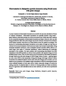
FIG. 1. Radial distribution functions g(r) as obtained in DPD simulations of the 3D ideal gas for ∆t = 0.01 (left) and ∆t = 0.1 (right) for velocity–Verlet–based integrators. Time p is given in units of rc m/kB T .

ideal

~ =κ /κ κ T T T

0.58

0.90

0.80

0.56

0.75 0.70 0.01

DT MD-VV

0.54

DPD-VV self-consist. DPD-VV

0.1

∆t

0.01

0.1

0.1

vealed that their results were approximately similar to those of MD–VV and DPD–VV, respectively. For all integrators, the artificial structure in g(r) becomes more pronounced with increasing time increment ∆t, and it is intriguing that the bias introduced by the self–consistent integrator for ∆t = 0.10 is comparable to that introduced by MD–VV for ∆t = 0.01. The relative isothermal compressibilities e κT evaluated from g(r) are shown in Fig. 2. The qualitative behavior of κ eT reflects our findings for g(r) [16]. However, the magnitude of deviations from κ eT = 1 is astounding, and raises serious concern for studies of response functions such as the compressibility for interacting fluids close to phase boundaries. Similarly, the results for tracer diffusion (also in Fig. 2) indicate that DPD–VV and the self–consistent approach work well up to reasonably large time steps, while the other integrators were found to perform less well. Thus, the decay of velocity correlations in tracer diffusion is sensitive to the choice of the integrator. These results demonstrate that special care is needed in studies of DPD model systems, and suggest that integrators commonly used in MD should not be employed in DPD as such. Next we discuss the deviations of the observed actual temperature hkB T i from the desired temperature kB T ∗ (see Fig. 3). For MD–VV this “temperature drift” is always positive and increases monotonically with ∆t. For DPD–VV, hkB T i first decreases with increasing ∆t, then exhibits a minimum at ∆t ≈ 0.25, and eventually becomes larger than kB T ∗ . The self–consistent approach exhibits a negative, monotonically increasing temperature drift up to ∆t ≈ 0.13, where this scheme becomes unstable at the employed particle density. Most importantly, we find, surprisingly, that the modulus of the temperature deviation is even larger than the one for DPD–VV. In a recent work, Pagonabarraga et al. [8] studied the 2D ideal gas using a self–consistent version of the leap–frog algorithm, and found good temperature control for ∆t = 0.06 at ρ = 0.5. This discrepancy can be explained by our observation for the 3D ideal gas that the temperature drift is in general more pronounced at higher densities.

1.00

0.85

∆t

FIG. 3. Double–logarithmic plot of the modulus of the deviation of from the desired temperature kB T ∗ ≡ 1 vs. ∆t. For self–consistent DPD–VV with auxiliary thermostat, 1σ error bars are shown for some of the data points.

10 × 10 × 10 with periodic boundary conditions, a random force strength σ = 3 , and a particle density ρ = 4 (i.e., N = 4000 particles) [14]. For the equilibrated system, the temperature hkB T i and the radial distribution function g(r) were sampled. For the ideal gas, g(r) ≡ 1 in the continuum limit, and therefore any deviation from 1 has to be interpreted as an artifact due to the employed integration scheme. Artifacts in g(r) are also reflected in the relative isothermal compressibility κ eT ≡ κT /κideal , where κideal = (ρ kB T ∗ )−1 denotes the T T compressibility of the ideal gas in the continuum limit. For an Rarbitrary fluid, κ eT is related to g(r) by κ eT = ∞ 1 + 4πρ 0 dr r2 [g(r) − 1] , and thus any deviation from κ eT = 1 for the ideal gas indicates an integrator–induced artifact. Finally, to gauge underlying problems in the actual dynamics of the system, we consider the tracer diffuPN 1 2 sion coefficient DT = limt→∞ 6N i=1 h[ri (t) − ri (0)] i, t which characterizes temporal correlations between the displacements (velocities) of the tagged particle. Results for g(r) are shown in Fig. 1. We find that the deviations from g(r) = 1 are very pronounced for MD– VV, indicating that even at small time steps it gives rise to unphysical correlations. The performance of DPD–VV is clearly better, while the self–consistent scheme leads to even smaller deviations. Studies of the integrators GW(λ = 0.65) and GCC(λ) (for a few values of λ) re-

0.95

0.01

0.52

∆t

FIG. 2. Left: Dimensionless isothermal compressibility κ eT vs. ∆t for the integrators shown in the legend. Right: Tracer diffusion coefficient DT vs. ∆t for the same integrators.

3

whether DPD is able to describe the dynamics and transport properties of complex fluids [4,8]. Since the origin of the observed discrepancies is not clear and a general theory is still lacking, it will be interesting to see what the impact of the ideas presented here is on transport properties. Work is in progress to address these questions [15]. This work was supported by the Danish Natural Science Research Council (G.B.), a European Union grant (I.V.), and the Natural Sciences and Engineering Research Council of Canada (J.M.P.).

In cases where temperature preservation is crucial in calculating equilibrium quantities, we finally demonstrate how this can be achieved. The idea is to supplement the self–consistent scheme by an auxiliary thermostat, which preserves the pairwise conservation of momentum by employing a fluctuating dissipation strength γ(t) =

σ2 (1 + η(t) ∆t) , 2 kB T ∗

(3)

where η is a thermostat variable. The rate of change of η is proportional to the instantaneous temperature deviation, η˙ = C(kB T−kB T ∗ ) , where C is a coupling constant (step (i) in Table II) [17]. This first–order differential equation must be integrated (step (ii)) simultaneously with the equations of motion. In this respect our thermostat resembles the Nos´e–Hoover thermostat familiar from MD simulations [13]. For this extended–system method, we find (Fig. 3) that the temperature deviations diminish by over two orders of magnitude, with a modulus typically of the order of 10−5 . . . 10−4 . We also found virtually the same results for g(r) and e κT as for the self–consistent scheme without the thermostat. This suggests that the auxiliary thermostat is useful in studies of equilibrium quantities such as the speficic heat. However, we feel that the auxiliary thermostat is not an ideal approach to describe quantitative aspects of tracer diffusion. A more detailed study is currently in progress [15]. In this work, we have shown that integration schemes may in DPD lead to pronounced artifacts in response functions and transport coefficients. This constitutes a serious problem for studies of soft systems, and highlights the timely need to resolve this issue. We have demonstrated that these artifacts can be sufficiently suppressed by using velocity–Verlet–based schemes in which the velocity dependence of the dissipative forces is taken into account. The velocity–Verlet scheme without iterations but with an additional update of the dissipative forces (DPD–VV) performs — at essentially unchanged computational costs — already considerably better than the Groot–Warren integrator. The best overall performance is found for a recently proposed approach [8], in which particle velocities and velocity–dependent dissipative forces are determined self–consistently. This scheme provides an accurate description for the quantities studied here, except for the temperature whose persisting drift is found to be unexpectedly significant. As shown in this work, however, this drift can be suppressed by at least two orders of magnitude by a scheme which supplements self–consistency with an auxiliary thermostat. The computational cost of the self–consistent scheme without thermostat remains modest, and increases only by a factor of 1.5 to 3 with respect to the standard velocity– Verlet algorithm. Although DPD has been very successful especially in simulations of polymeric systems and in reproducing equilibrium properties, there have been doubts as to

∗

[1] [2] [3]

[4] [5] [6] [7] [8] [9] [10] [11]

[12] [13] [14] [15] [16]

[17]

4

Corresponding author. Present address: Max Planck Institute for Polymer Research, Mainz, Germany. Electronic address: besold@mpip–mainz.mpg.de . P. J. Hoogerbrugge and J. M. V. A. Koelman, Europhys. Lett. 19, 155 (1992). P. Espa˜ nol and P. Warren, Europhys. Lett. 30, 191 (1995). E. G. Flekkøy and P. V. Coveney, Phys. Rev. Lett. 83, 1775 (1999); A. J. C. Ladd, Phys. Rev. Lett. 70, 1339 (1993); M. Murat and K. Kremer, J. Chem. Phys. 108, 4340 (1998). R. D. Groot and P. B. Warren, J. Chem. Phys. 107, 4423 (1997). P. B. Warren, Curr. Opin. Colloid. Interf. Sci. 3, 620 (1998). K. E. Novik and P. V. Coveney, J. Chem. Phys. 109, 7667 (1998). C. A. Marsh and J. M. Yeomans, Europhys. Lett. 37, 511 (1997). I. Pagonabarraga, M. H. J. Hagen, and D. Frenkel, Europhys. Lett. 42, 377 (1998). J. B. Gibson, K. Chen, and S. Chynoweth, Int. J. Mod. Phys. C 10, 241 (1999). C. A. Marsh, G. Backx, and M. H. Ernst, Europhys. Lett. 38, 411 (1997). C. A. Marsh, G. Backx, and M. H. Ernst, Phys. Rev. E 56, 1676 (1997); G. T. Evans, J. Chem. Phys. 110, 1338 (1999); R. D. Groot, T. J. Madden, and D. J. Tildesley, J. Chem. Phys. 110, 9739 (1999). L. Verlet, Phys. Rev. 159, 98 (1967). J. M. Thijssen, Computational Physics (Cambridge University Press, Cambridge, 1999). As basic units we use the particle mass m, the cut–off length rc , and the desired equilibrium temperature kB T ∗ . I. Vattulainen et al., in preparation. However, for ∆t > ∼ 0.3 the positive and negative deviations of g(r) from 1 accidentally almost cancel each other for both MD-VV and DPD-VV. Self–consistent DPD-VV becomes unstable (no convergence anymore) at ∆t ≈ 0.13 for the density ρ = 4 . The coupling constant C has to be chosen with care. For the simulations reported here, we always ensured that the employed values of C did not cause any bias.