LS-SVMlab: a MATLAB/C toolbox for Least Squares Support Vector ...

LS-SVMlab: a MATLAB/C toolbox for Least Squares Support Vector Machines

Kristiaan Pelckmans, Johan A.K.Suykens, T. Van Gestel, J. De Brabanter, L. Lukas, B. Hamers, B. De Moor and J.Vandewalle ESAT-SCD-SISTA K.U. Leuven Kasteelpark Arenberg 10 B-3001 Leuven-Heverlee, Belgium kristiaan.pelckmans,johan.suykens @esat.kuleuven.ac.be




Abstract In this paper, a toolbox LS-SVMlab for Matlab with implementations for a number of LS-SVM related algorithms is presented. The core of the toolbox is a performant LS-SVM training and simulation environment written in C-code. The functionality for classification, function approximation and unsuperpervised learning problems as well time-series prediction is explained. Extensions of LS-SVMs towards robustness, sparseness and weighted versions, as well as different techniques for tuning of hyper-parameters are included. An implementation of a Bayesian framework is made, allowing probabilistic interpretations, automatic hyperparameter tuning and input selection. The toolbox also contains algorithms of fixed size LS-SVMs which are suitable for handling large data sets. A recent overview on developments in the theory and algorithms of least squares support vector machines to which this LS-SVMlab toolbox is related is presented in [1].

1 Introduction Support Vector Machines (SVM) [2, 3, 4, 5] is a powerful methodology for solving problems in nonlinear classification, function estimation and density estimation which has also led to many other recent developments in kernel based methods in general. Originally, it has been introduced within the context of statistical learning theory and structural risk minimization. In the methods one solves convex optimization problems, typically by quadratic programming. Least Squares Support Vector Machines (LS-SVM) are re-formulations to the standard SVMs [6, 7]. The cost function is a regularized least squares function with equality constraints, leading to linear Karush-Kuhn-Tucker systems. The solution can be found efficiently by iterative methods like the Conjugate Gradient (CG) algorithm [8]. LSSVMs are closely related to regularization networks, Gaussian processes [9] and kernel fisher discriminant analysis[10], but additionally emphasize and exploit primal-dual interpretations. Links between kernel versions of classical pattern recognition algorithms and extensions to recurrent networks and control [11] and robust modeling [12, 13] are available. A Bayesian evidence framework has been applied with three levels of inference 

http://www.esat.kuleuven.ac.be/sista/lssvmlab

LS−SVMlab Toolbox Matlab/C Basic

Advanced Bayesian framework

C−code

model validation

lssvm MATLAB

bay_lssvm bay_optimize

NAR(X) & prediction

demos model tuning

tunelssvm prunelssvm weightedlssvm

code code_ECOC

lssvm.mex* lssvm.x

trainlssvm

crossvalidate leaveoneout

simlssvm plotlssvm

validate

kpca

encoding

predict preprocessing

windowize

prelssvm postlssvm

windowizeNARX

Fixed Size LS−SVM AFE kentropy ridgeregress bay_rr

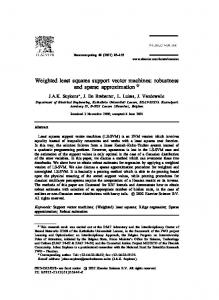
Figure 1: Schematic illustration of the organization of LS-SVMlab. Each box contains the names of the corresponding algorithms. The function names with extension “lssvm” are LS-SVM method specific. The dashed box includes all functions of a more advanced toolbox, the large grey box those that are included in the basic version.

[14], allowing for probabilistic interpretations, automatic hyper-parameter selection, model comparison and input selection. Recently, a number of methods [1] and criteria are presented for the extension of LS-SVM training techniques towards large datasets, including a method of fixed sise LS-SVM which is related to a Nystr¨om sampling with active selection of support vectors and estimation in the primal space. This paper is organized as follows. In Section 2 we present the main ideas behind LSSVMlab. For the exact syntax of the function calls, we refer to the website and the Matlab help. Section 3 illustrates the principles of fixed size LS-SVM for large scale problems. This paper concludes with some final remarks. References to commands in the toolbox are made in the typewriter font.

2 A birds eye view on LS-SVMlab The toolbox is mainly intended for use with the commercial Matlab package. However, the core functionality is written in C-code. The Matlab toolbox is compiled and tested for different computer architectures including Linux, Windows and Solaris. Most functions can handle datasets up to 20.000 data points or more. LS-SVMlab’s interface for Matlab consists of a basic version for beginners as well as a more advanced version with programs for multi-class encoding techniques and a Bayesian framework. Future versions will gradually incorporate new results and additional functionalities. The organization of the toolbox is schematically shown in Fig.1. A number of functions are restricted to LS-SVMs (these include the extension “lssvm” in the function name), the others are generally usable. A number of demos illustrates how to use the different features of the toolbox. The Matlab function interfaces are organized in 2 principal ways: the functions can be called either in a functional way or using an object alike structure (referred to as the model) as e.g. in Netlab [15], depending on the user’s choice. For other implementations of kernel related techniques, see 1 . 1

http://www.kernel-machines.org/software.html

4

3

CMEX CFILE MATLAB

3

class 1 class 2 class 3 2

2

10

2 1

1 2

10

X2

seconds needed on a PIII 833Mhz linux PC

10

1 2

0

1

10

2

−1

0

10

−2

132 164

228

356

612

1124

2148

4196

size dataset

8292

2 1

−3 −4

−3

−2

−1

0

1

2

X

1

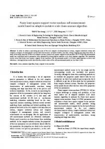
Figure 2: (Left) Indication of the performance for the different training implementations of LS-SVMlab; (Right) LS-SVM multiclass example with one-versus-one encoding;

2.1 Classification and Regression: trainlssvm, simlssvm, plotlssvm The Matlab toolbox is built around a fast LS-SVM training and simulation algorithm. The corresponding calls can be used for classification as well as for function estimation. The function plotlssvm displays the simulation results of the model in the region of the training points. To avoid failures and ensure performance of the implementation, three different implementations are included. The most performant is the CMEX implementation (lssvm.mex*), based on C-code linked with Matlab via the CMEX interface. More reliable is the Ccompiled executable (lssvm.x) which passes the parameters to/from Matlab via a buffer file. Both use the fast conjugate gradient algorithm to solve the set of linear equations [8]. The C-code for training takes advantage of previously calculated solutions. Less performant but stable, flexible and straightforward coded is the implementation in Matlab (lssvmMATLAB.m) based on the Matlab matrix division backslash command . Functions for single and multiple output regression and classification are available. Training and simulation can be done for each output separately by passing different kernel functions, kernel and/or regularization parameters as a column vector. It is straightforward to implement other kernel functions in the toolbox. The performance of a model depends on the scaling of the input and output data. An appropriate algorithm detects and appropriately rescales continuous, categorical and binary variables (prelssvm, postlssvm). 2.2 Classification Extensions: codelssvm, code, deltablssvm, roc A number of additional function files are available for the classification task. The Receiver Operating Characteristic curve (roc) can be used to measure the performance of a classifier. Multiclass classification problems are decomposed into multiple binary classification tasks [16]. Several coding schemes can be used at this point: minimum output, one-versus-one, one-versus-all and error correcting coding schemes. To decode a given result, the Hamming distance, loss function distance and Bayesian decoding can be applied. A correction of the bias term can be done, which is especially interesting for small data sets. Example 1: multiclass coding (Fig.2.right)

LS−SVM 2.5

2

γ:16243.8705,σ :6.4213

β

tuned by classical L V−fold CV, 2

2.5

model noise: F(e) = (1−ε) N(0,0.12)+ε N(0,1.52)

LS−SVM data points real function

2

2

2

LS−SVM data points real function

2

1.5

1.5

1

1

0.5

0.5

0

0

−0.5

−0.5

−1

−1

−1.5

−1.5

−2

−2.5 −5

LS−SVMγ:6622,7799,σ2:3.7563 tuned by repeated CVrobust , model noise: F(e) = (1−ε) N(0,0.1 )+ε N(0,1.5 )

−2

−4

−3

−2

−1

0

1

2

3

4

5

−2.5 −5

−4

−3

−2

−1

X

0

1

2

3

4

5

X

Figure 3: Experiments on a noisy sinc dataset with 15% outliers. (Left) Application of the standard training and hyperparameter estimation techniques; (Right) Application of a weighted LS-SVM training together with a robust crossvalidation score function, which enhances the test set performance.

>> >> >> >> >> >>

% load multiclass data X and Y... [Ycode,codebook,oldcodebook] = code(Y, ’code_OneVsOne’); [gam,sig2] = tunelssvm({X,Ycode,’class’,1,1}); [alpha,b] = trainlssvm({X,Ycode,’class’,gam,sig2}); Ytest_coded = simlssvm({X,Ycode,’class’,gam,sig2},{alpha,b},Xtest); Ytest = code(Ytest_coded, oldcodebook, codebook, ’codedist_hamming’);

2.3 Tuning, Sparseness, Robustness:tunelssvm,validate, crossvalidate, rcrossvalidate, leaveoneout, weightedlssvm, prunelssvm A number of methods to estimate the generalisation performance of the trained model are included. The estimate of the performance based on a fixed testset is calculated by validate. For classification, the rate of misclassifications (misclass) can be used. Estimates based on repeated training and validation are given by crossvalidate and leaveoneout. The implementation of those include a bias correction term. A robust crossvalidation score function [13] is called by rcrossvalidate. These performance measures can be used to tune the hyper-parameters (e.g. the regularization and kernel parameters) of the LS-SVM (tunelssvm). Reducing the model complexity of a LS-SVM can be done by iteratively pruning the less important support values (prunelssvm) [12]. In the case of outliers in the data or non-Gaussian noise, corrections to the support values will improve the model (weightedlssvm) [12].

2.4 Bayesian Framework: bay lssvm, bay optimize, bay lssvmARD, bay errorbar, bay modoutClass Functions to calculate the posterior probability of the model and hyper-parameters at different levels of inference are available (bay_lssvm). Errors bars are obtained by taking into account modeland hyper-parameter uncertainties (bay_errorbar). For classification [14], one can estimate the moderated output (bay_modoutClass). The Bayesian framework makes use of the eigenvalue decomposition of the kernel matrix. The size of the matrix grows with the number of data points. Hence, one needs approximation techniques to handle large datasets. It is known that mainly the principal eigenvalues and corresponding eigenvectors are relevant. Therefore, iterative approximation methods as the Nystr¨om method [17, 18] are included, which is also frequently used in Gaussian processes. Input selection can be done by Automatic Relevance Determination (bay_lssvmARD)

300

class 1 class 2

1.2

250 1

0.8

200

Y

X2

0.6 150

0.4 100 0.2

50

0

−0.2 −1

−0.5

0

0.5

X1

1

0

0

10

20

30

40

50 time

60

70

80

90

100

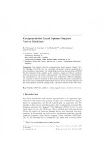
Figure 4: (Left) Moderated output of the LS-SVM classifier on the Ripley data set. Shown are lines of equal posterior class probability. (Right) Santa Fe chaotic laser data (-); iterative prediction using LS-SVMs (- -). [19]. In this backward variable selection, the third level of inference of the Bayesian framework is used to infer the most relevant dimensions of the problem. Example 2: LS-SVM classifier on the Ripley data set (Fig.4.left) >> % load dataset X and Y... >> [gam,sig2] = tunelssvm({X,Y,’class’,1,1},... ’gridsearch’,{},’crossvalidate’,{X,Y,10,’misclass’}); >> [alpha,b] = trainlssvm({X,Y,’class’,gam,sig2}); >> plotlssvm({X,Y,’class’,gam,sig2},{alpha,b}); >> Ymodout = bay_modoutClass({X,Y,’class’,gam,sig2},Xtest);

2.5 NARX Models and Prediction: predict, windowize Extensions towards nonlinear NARX systems for time series applications are available [1]. A NARX model can be built based on a nonlinear regressor by estimating in each iteration the next output value given the past output (and input) measurements. A dataset is converted into a new input (the past measurements) and output set (the future output) by windowize and windowizeNARX for respectively the time series case and in general the NARX case with exogenous input. Iteratively predicting (in recurrent mode) the next output based on the previous predictions and starting values is done by predict.

Example 3: Santa Fe laser data prediction (Fig.4.right) >> % load timeseries X; delays = 50; >> Xu = windowize(X,1:delays+1); >> [gam,sig2] = tunelssvm({Xu(:,1:delays),Xu(:,end),... ’function’,1,1,’RBF_kernel’}); >> [alpha,b] = trainlssvm({Xu(:,1:delays),Xu(:,end),... ’function’,gam,sig2,’RBF_kernel’}); >> prediction = predict({Xu(:,1:delays),Xu(:,end),... ’function’,gam,sig2,’RBF_kernel’},X(1:delays),100);

2.6 Unsupervised Learning: kpca Unsupervised learning can be done by kernel based PCA (kpca) as described by [20], for which recently a primal-dual interpretation with support vector machine formulation has been given in [21], which can also be further extended to kernel canonical correlation analysis [1].

Criterion Fixed size selected subset

Regression in primal space

Y Training data set

ϕ(.)

X

Figure 5: Fixed Size LS-SVM is a method for modeling large scale regression and classification problems. The number of support vectors is pre-fixed beforehand and the support vectors are selected from a pool of training data. After estimating eigenfunctions in relation to a Nystr¨om sampling with selection of the support vectors according to an entropy criterion, the LS-SVM model is estimated in the primal space.

3 Solving large scale problems with fixed size LS-SVM Classical kernel based algorithms like e.g. LS-SVM [6] typically have a complexity of memory and calculations larger than . Recently, work on large scale methods proposes solutions to circumvent this bottleneck [1, 20].




For large datasets it would be advantageous to solve the least squares problem in primal weight space as then the size of the vector of unknowns is proportional to the feature vector dimension and not to the number of datapoints. However, the feature space mapping induced by the kernel is needed in order to obtain non-linearity. For this purpose, a method of fixed size LS-SVM is proposed [1] (see fig. 5). Firstly the Nystr¨om method [18, 14] can be used to estimate the feature space mapping. The link between Nystr¨om sampling, kernel PCA and density estimation has been discussed in [22]. In fixed size LS-SVM these links are employed together with the explicit primal-dual LS-SVM interpretations. The support vectors are selected according to an entropy criterion (kentropy). In a last step a regression is done in the primal space which makes the method suitable for solving large scale nonlinear function estimation and classification problems. A Bayesian framework for ridge regression [23, 14] (bay_rr) can be used to find the optimal regularization parameter. Example 4: Fixed Size LS-SVM (Fig.6.right) >> >> >> >>

% load data X and Y, the capapcity and the kernel parameter sig2 sv = 1:capacity; max_c = -inf; for i=1:size(X,1), replace = ceil(rand.*capacity); subset = [sv([1:replace-1 replace+1:end]) i]; crit = kentropy(X(subset,:),’RBF_kernel’,sig2); if max_c> features = AFE(svX,’RBF_kernel’,sig2, X); >> [Cl3, gam_optimal] = bay_rr(features,Y,1,3); >> [W,b, Yh] = ridgeregress(features, Y, gam_opt); An alternative criterion for subset selection was presented by [24, 25], which is closely related to [18] and [20]. It measures the quality of approximation of the feature space and the space induced by the subset (featvecsel). Originally [18], the subset was taken as a independent and identiquely

estimated costsurface of fixed size LS−SVM based on repeated iid. subsampling

fixed size LS−SVM on 20.000 noisy sinc datapoints

1.4

training data estimated function real function data of subset

1.2

0.12 1 0.1 0.8 cost

0.08

0.6

0.06 0.04

Y

0.4 0.02 0.2

0 1

0 21 −0.2 46

1024 16

−0.4

71 0.0625

−0.6 −5

−4

−3

−2

−1

0 X

1

2

3

4

5

capacity subset

96

0.000976562 2

σ

Figure 6: Illustration of fixed size LS-SVM on a noisy sinc function with 20000 data points: (Left) Fixed size LS-SVM selects a subset of the data to approximate the implicit mapping to the feature space. The regularization parameter for the regression in primal space is optimized here using the bayesian framework; (Right) Estimated cost surface of the fixed size LS-SVM based on repeated i.i.d. subsamples of the data, of different subset capacities and kernel parameters. The cost is measured on a validation set. distributed (i.i.d.) subsample from the data (subsample), which can be used for fast and rough performance optimization.

4 Final Remarks In this paper a Matlab/C toolbox has been proposed. It combines the flexibility of Matlab with the efficiency of C-code and numerically stable algorithms suitable for solving larger scale problems. The toolbox is offered to researchers and practitioners in LS-SVMs and the broad area of support vector machines, regularization networks, Gaussian processes and kernel based methods, where it may also be suitable for comparative tests. Acknowledgements Our research is supported by grants from several funding agencies and sources: Research Council K.U. Leuven: Concerted Research Action GOAMefisto 666 (Mathematical Engineering), IDO (IOTA Oncology, Genetic networks), several PhD/postdoc & fellow grants; Flemish Government: Fund for Scientific Research FWO Flanders (several PhD/postdoc grants, projects G.0407.02 (support vector machines), G.0080.01 (collective intelligence), G.0256.97 (subspace), G.0115.01 (bio-i and microarrays), G.0240.99 (multilinear algebra), G.0197.02 (power islands), research communities ICCoS, ANMMM), AWI (Bil. Int. Collaboration Hungary/Poland), IWT (Soft4s (softsensors), STWW-Genprom (gene promotor prediction), GBOU McKnow (Knowledge management algorithms), Eureka-Impact (MPC-control), Eureka-FLiTE (flutter modeling), several PhD grants); Belgian Federal Government: DWTC (IUAP IV-02 (1996-2001) and IUAP V-10-29 (2002-2006): Dynamical Systems and Control: Computation, Identification & Modelling), Program Sustainable Development PODO-II (CP-TR-18: Sustainibility effects of Traffic Management Systems); Direct contract research: Verhaert, Electrabel, Elia, Data4s, IPCOS. JS is a professor at K.U.Leuven Belgium and a postdoctoral researcher with FWO Flanders. BDM and JWDW are a full professor at K.U.Leuven Belgium.

References [1] Suykens J.A.K., Van Gestel T., De Brabanter J., De Moor B., Vandewalle J., Least Squares Support Vector Machines, World Scientific, to appear. [2] Cristianini N., Shawe-Taylor J., An Introduction to Support Vector Machines, Cambridge University Press, 2000. [3] Sch¨olkopf B., Burges C., Smola A. (Eds.), Advances in Kernel Methods - Support Vector Learning, MIT Press, 1998. [4] Sch¨olkopf, B. and Smola A., Learning with Kernels, MIT Press, Cambridge MA, 2002.

[5] Vapnik V., Statistical learning theory, John Wiley, New-York, 1998. [6] Suykens J.A.K., Vandewalle J., “Least squares support vector machine classifiers,” Neural Processing Letters, 9(3), 293-300, 1999. [7] Van Gestel T., Suykens J., Baesens B., Viaene S., Vanthienen J., Dedene G., De Moor B., Vandewalle J., “Benchmarking Least Squares Support Vector Machine Classifiers ”, Machine Learning, in press. [8] Hamers B., Suykens J.A.K., De Moor B., “A comparison of iterative methods for least squares support vector machine classifiers”, Internal Report 01-110, ESAT-SISTA, K.U.Leuven (Leuven, Belgium), 2001. [9] Evgeniou T., Pontil M., Poggio T., “Regularization networks and support vector machines,” Advances in Computational Mathematics, 13(1), 1-50, 2000. [10] Mika S., R¨atsch G., Weston J., Sch¨olkopf B., M¨uller K.-R. (1999) “Fisher discriminant analysis with kernels”, In Y.-H. Hu, J. Larsen, E. Wilson, and S. Douglas, editors, Neural Networks for Signal Processing IX, 41-48. IEEE. [11] Suykens J.A.K., Vandewalle J., “Recurrent least squares support vector machines”, IEEE Transactions on Circuits and Systems-I, 47(7), 1109-1114, 2000. [12] Suykens J.A.K., De Brabanter J., Lukas L., Vandewalle J., “Weighted least squares support vector machines : robustness and sparse approximation”, Neurocomputing, in press. [13] De Brabanter J., Pelckmans K., Suykens J.A.K., Vandewalle J., “Robust cross-validation score function for non-linear function estimation”, International Conference on Artificial Neural Networks (ICANN 2002), Madrid Spain, to appear, 2002 [14] Van Gestel T., Suykens J.A.K., Lanckriet G., Lambrechts A., De Moor B., Vandewalle J., “Bayesian Framework for Least Squares Support Vector Machine Classifiers, Gaussian processes and kernel Fisher discriminant analysis”, Neural Computation, 15(5), 1115-1148, 2002. [15] Nabney I.T., Netlab: Algorithms for Pattern Recognition Springer, 2002. [16] Van Gestel T., Suykens J.A.K., Lanckriet G., Lambrechts A., De Moor B., Vandewalle J., “Multiclass LS-SVMs : Moderated outputs and coding-decoding schemes”, Neural Processing Letters, 15(1), 45-58, 2002. [17] Van Gestel T., Suykens J.A.K., De Moor B., Vandewalle J., “Bayesian inference for LS-SVMs on large data sets using the Nystr¨om method”, International Joint Conference on Neural Networks (IJCNN 2002), Honolulu, Hawaii, 2002. [18] Williams C. and Seeger M., “Using the Nystrom method to speedup kernel machines”, NIPS 13, MIT Press, 2001. [19] Van Gestel T., Suykens J.A.K., De Moor B., Vandewalle J., “Automatic relevance determination for least squares support vector machine classifiers”, Proc. of the European Symposium on Artificial Neural Networks (ESANN 2001), Bruges, Belgium, pp. 13-18, 2001. [20] Smola A. and Schlkopf B., “Sparse greedy matrix approximation for machine learning”, International Conference on Machine Learning, 2000. [21] Suykens J.A.K., Van Gestel T., Vandewalle J., De Moor B., “A support vector machine formulation to PCA analysis and its Kernel version”, Internal Report 02-68, ESAT-SISTA, K.U.Leuven (Leuven, Belgium), 2002. [22] Girolami M., “Orthogonal Series Density Estimation and the Kernel Eigenvalue Problem”. Neural Computation, MIT Press, 14(3), 669-688, 2002. [23] MacKay D.J.C. “Bayesian interpolation”, Neural Computation, 4(3), 415–447, 1992. [24] Baudat G., and Anouar F., “Kernel-based Methods and Function Approximation” International Joint Conference on Neural Networks (IJCNN 2001), Washington DC USA, pp.1244-1249, 2001. [25] Cawley G.C., Talbot N.L.C., “Efficient formation of a basis in a kernel induced feature space”, Proc. European Symposium on Artificial Neural Networks (ESANN 2002), Brugge Belgium, pp.1-6, 2002.