Jan 13, 2008 - *School of Operations Research & Information Engineering, Cornell University, Ithaca, New York 14853. Research supported by a DOE ...
MNH: A Derivative-Free Optimization Algorithm Using Minimal Norm Hessians Stefan M. Wild∗ January 13, 2008 Abstract We introduce MNH, a new algorithm for unconstrained optimization when derivatives are unavailable, primarily targeting applications that require running computationally expensive deterministic simulations. MNH relies on a trust-region framework with an underdetermined quadratic model that interpolates the function at a set of data points. We show how to construct this interpolation set to yield computationally stable parameters for the model and, in doing so, obtain an algorithm which converges to first-order critical points. Preliminary results are encouraging and show that MNH makes effective use of the points evaluated in the course of the optimization.
1
Introduction
In this paper we address unconstrained optimization, min {f (x) : x ∈ Rn } ,
(1.1)
of a function whose derivatives are unavailable. Our work is motivated by functions that are computationally expensive to evaluate, usually as a result of the need to run some underlying complex simulation model. These simulations often provide the user solely with the simulation output, creating the need for a derivative-free optimization algorithm. Examples of derivativefree optimization applied to these types of problems in electrical, environmental, and medical engineering can be found in [6, 8, 13]. When f is computationally expensive, a user is typically constrained by a computational budget that limits the number of function evaluations available to the optimization algorithm. We view the data gained from each function evaluation as contributing to a bank of insight into the function. As the optimization is carried out, more points are evaluated and this bank will grow. How to most effectively manage the data contained in the bank is a central driving force behind this paper. Our approach is inspired by the recent work of Powell [10, 11] using quadratic models interpolating fewer than a quadratic (in the dimension n) number of points. This strategy allows the underlying optimization to begin sooner and make more rapid progress in fewer function evaluations. These models are assumed to locally approximate the function while being computationally inexpensive to evaluate and optimize over. In this paper we introduce a new algorithm, MNH, that contributes two new features. First, unlike previous algorithms [8, 11], which were driven by a desire to keep linear algebraic overhead to O(n3 ) operations per iteration, our algorithm views overhead as negligible relative to the expense of function evaluation. This allows greater flexibility in using points from the bank. Second, our models are formed from interpolation sets in a computationally stable manner which guarantees that the models are well-behaved. In fact, both our model and its gradient are able to approximate the function and its gradient arbitrarily well. Consequently, the recent convergence ∗
School of Operations Research & Information Engineering, Cornell University, Ithaca, New York 14853. Research supported by a DOE Computational Science Graduate Fellowship under grant number DE-FG02-97ER25308
1
result of Conn, Scheinberg and Vicente [3] guarantees that our algorithm will converge to first-order critical points. Encouraged by preliminary results, we hope that this convergence result and our way of using points from the bank will yield a theoretically sound algorithm that is both relatively simple and works well in practice. This paper is organized as follows. In Section 2 we review derivative-free trust-region algorithms. Section 3 introduces the special quadratic models employed by our algorithm. The MNH algorithm is provided in Section 4 and preliminary numerical findings are presented in Section 5.
2
Derivative-Free Trust-Region Methods
Our algorithm is built upon a trust-region framework that we now review. A trust-region method is an iterative method that optimizes over a surrogate model mk assumed to approximate f within a neighborhood of the current iterate xk , the trust-region Bk = {x ∈ Rn : kx − xk k ≤ ∆k }, for a radius ∆k > 0. New candidate points are obtained by solving the subproblem min {mk (xk + s) : xk + s ∈ Bk } .
(2.1)
In fact, it suffices to only solve (2.1) approximately, provided that the resulting step sk satisfies a sufficient decrease condition. The pair (xk , ∆k ) is updated according to the ratio of actual to predicted decrease, f (xk ) − f (xk + sk ) , ρk = mk (xk ) − mk (xk + sk ) ρk values close to 1 corresponding to good model prediction. A quadratic model, 1 mk (xk + s) = f (xk ) + gkT s + sT Hk s, 2
(2.2)
is typically employed with gk = ∇f (xk ) and Hk = ∇2 f (xk ) when these derivatives are available. The quadratic model in (2.2) is attractive because global solutions to the subproblem in (2.1) can then be efficiently computed. When the gradient ∇f is exactly available, global convergence to local minima is possible under mild assumptions. Full treatment is given in [1]. Given an initial point x0 and a maximum radius ∆max , the design of the trust-region algorithm ensures that f is only sampled within the relaxed level set L(x0 ) = {y ∈ Rn : kx − yk ≤ ∆max for some x with f (x) ≤ f (x0 )}. When only function values are available, the model mk can be obtained by interpolating the function at a set of distinct data points Y = {y1 = 0, y2 , . . . , y|Y| } ⊂ Rn : mk (xk + yj ) = f (xk + yj )
for all yj ∈ Y.
(2.3)
This approach was taken with both quadratic [2, 9] and radial basis function (RBF) models [8, 13]. A primary concern in the study of interpolation model-based derivative-free methods is the quality of the model within Bk . In [4], Taylor-like error bounds are established based on the geometry of the interpolation set Y. These results motivate a class of so-called fully linear models for approximating functions that are reasonably smooth. In particular, we will assume that f ∈ C 1 [Ω] for some open Ω ⊃ L(x0 ), ∇f is Lipschitz continuous on L(x0 ), and f is bounded on L(x0 ). 2
Definition 1. For fixed κf , κg > 0 and B = {x ∈ Rn : kx − xk k ≤ ∆}, a model m ∈ C 1 [Ω] is said to be fully linear (f.l.) on B if for all x ∈ B: |f (x) − m(x)| ≤ κf ∆2 ,
k∇f (x) − ∇m(x)k ≤ κg ∆.
(2.4) (2.5)
The two conditions in Definition 1 ensure that approximations to the true function and its gradient can achieve any desired degree of precision within a small enough neighborhood of xk . Provided that mk can be made fully linear for fixed κf and κg in finitely many steps, Algorithm 2.1 was recently shown to be globally convergent to a stationary point ∇f (x∗ ) = 0, given an appropriate termination test [3]. Input x0 ∈ Rn , 0 < ∆0 ≤ ∆max , m0 , 0 ≤ η0 ≤ η1 < 1 (η1 6= 0), 0 < γ0 < 1 < γ1 , �g > 0. Iteration k ≥ 0: 1. If k∇mk k ≤ �g , test for termination. 2. Solve min{mk (xk + s) : ksk ≤ ∆} for sk and set x+ = xk + sk . k )−f (x+ ) 3. Evaluate f (x+ ) and ρk = mfk (x (xk )−mk (x+ ) and update the center: xk+1
x+ if ρk ≥ η1 = x if η1 > ρk > η0 and mk f.l. on B k + xk else.
4. If ρk < η1 and mk not f.l. on Bk , improve model by evaluating at a model-improving point. Hence or otherwise update model to mk+1 . 5. Update the trust-region radius min{γ1 ∆k , ∆max } if ρk ≥ η1 and ksk k ≥ ∆2k ∆k+1 = ∆ if ρk < η1 and mk not f.l. on Bk k γ0 ∆k if ρk < η1 and mk f.l. on B k . Algorithm 2.1: Basic first-order derivative-free trust-region algorithm.
3
Minimum Norm Quadratic Interpolation Models
In this paper we are interested in quadratic models of the form (2.2) with the parameters gk and Hk such that mk satisfies the interpolation conditions (2.3). To this end, we we define µ(x) = [1, χ1 , · · · , χn ] , � 2 � χ1 χ2n χ1 χ2 χn−1 χn ν(x) = , ··· , , √ , ··· , √ , 2 2 2 2 where χi denotes the ith component of the argument x ∈ Rn . When taken together, [µ(x), ν(x)] forms a basis for the linear space of quadratics in n variables, Qn . Thus any quadratic mk ∈ Qn can be written as mk (x − xk ) = αT µ(x − xk ) + β T ν(x − xk ), (3.1)
for coefficients α ∈ Rn+1 and β ∈ Rn(n+1)/2 . We note that any bijection of this basis would also yield a quadratic and so the form of the quadratic model in (3.1) may seem unusual at first glance. We propose to use this particular form of model because it lends itself well to our solution procedure. 3
Abusing notation, we let f denote the vector of function values so that (2.3) can be written as �
MY NY
�T �
α β
�
= f,
(3.2)
where we define MY ∈ Rn+1×|Y| and NY ∈ Rn(n+1)/2×|Y| , by Mi,j = µi (yj ) and Ni,j = νi (yj ), respectively. We explicitly note the dependence of these matrices on the interpolation set Y. The interpolation problem in (2.3) for multivariate quadratics is significantly more difficult than its univariate counterpart [12]. These points must satisfy additional geometric conditions that are summarized in the following Lemma, which follows immediately from the fact that [µ(x), ν(x)] form a basis for Qn . Lemma 3.1. The following are equivalent: 1. For any f ∈ R|Y| , there exists mk ∈ Qn satisfying (2.3). |Y| 2. {[µ(yj ), ν(yj )]}j=1 is linearly independent. 3. dim{q ∈ Qn : q(xk + yi ) = 0 ∀yj ∈ Y} =
(n+1)(n+2) 2
− |Y|.
The third condition in Lemma 3.1 reveals that these conditions are geometric, requiring that the subspace of quadratics disappearing at all of the data points be of sufficiently low dimension. For example, this prevents interpolation of arbitrary f values using 6 points lying on a circle in R2 . Lemma 3.1 implies that quadratic interpolation is only feasible for arbitrary right hand side values if [MYT , NYT ] is full row rank. Further, this interpolation is only unique if |Y| = (n+1)(n+2) 2 (the dimension of quadratics in Rn ) and [MYT , NYT ] is nonsingular. , and [MYT , NYT ] is full rank, (3.2) will have an infinite number of solutions. When |Y| < (n+1)(n+2) 2 In this paper we will focus on solutions to the interpolation problem (3.2) that are of minimum norm with respect to the vector β. Hence we require the solution (α, β) of � � 1 2 T T kβk : MY α + NY β = f . (3.3) min 2 This solution is of interest because it represents the quadratic whose Hessian matrix is of minimum Frobenius norm since kβk = k∇2x,x m(x)kF . While other “minimal norm” quadratics could be found, we are drawn to those with Hessians of minimal norm because the resulting solution procedure will have a natural tie-in to fully linear models. The KKT conditions for (3.3) can be written as �� � T � � � λ NY NY MYT f = , (3.4) MY 0 α 0 with β = NY λ. We solve this saddle point problem with a null space method by letting Z be an orthogonal basis for the null space N (MY ) and QR = MYT be a QR factorization. Since λ must belong to N (MY ), we write λ = Zω for ω ∈ R|Y|−n−1 so that (3.4) reduces to the |Y| equations: Z T NYT NY Zω = Z T f T
Rα = Q (f −
(3.5) NYT NY Zω),
(3.6)
with β = NY Zω. The following Theorem establishes that the quadratic program (3.3) will yield a unique solution given geometric conditions on Y. 4
Theorem 3.2. For n ≥ 2, if: (Y1) rank(MY ) = n + 1, and (Y2) Z T NYT NY Z is positive definite, then, for any f ∈ R|Y|, there exists a unique solution (α, β) to the quadratic program (3.3).
Proof. Z T NYT NY Z is positive definite if and only if NY Z is full rank. Since n ≥ 2, NY Z is full rank if and only if N (NY Z) = {0}. Lastly, since Z is a basis for N (MY ), this is equivalent to N (NY ) ∩ N (MY ) = {0}, which says that [MYT NYT ] is full rank. By Lemma 3.1, we then have that the feasible region of (3.3) is nonempty. Since (3.3) is a convex (in β) quadratic program whose feasible region is nonempty, both β and the Lagrange multipliers λ associated with the constraints are unique [5]. Finally, we note that the coefficients α are then also uniquely determined from MYT α = f − NYT β since MYT is full rank. If Z T NYT NY Z is positive definite, it admits the Cholesky factorization Z T NYT NY Z = LLT , for a nonsingular lower triangular L. Since Z is orthogonal we have the bound
2 kf k kλk = kZωk ZL−T L−1 Z T f ≤ L−1 kf k = 2 , σmin (L)
(3.7)
where σmin (L) is the smallest singular value of L. This relationship will allow us to bound the coefficients β = NY λ, and hence bound the Hessians of the model m.
4
The MNH Algorithm
Theorem 3.2 offers a constructive way of obtaining an interpolation set Y that uniquely defines an underdetermined quadratic model whose Hessian is of minimum norm. We first collect n + 1 affinely independent points and then add more points while keeping σmin (L) bounded from zero. We will always keep y1 = 0 in the set Y to enforce interpolation at the current center. Thus we only need to find n linearly independent points y2 , . . . , yn+1 . The resulting points will also serve a secondary purpose of providing approximation guarantees for the model m. This is formally stated in the following generalization of similar Taylor-like error bounds found in [4]. Theorem 4.1. Suppose that f and m are continuously differentiable in B = {x : kx−xk k ≤ ∆} and that ∇f and ∇m are Lipschitz continuous in B with Lipschitz constants γf and γm , respectively. Further suppose that m satisfies the interpolation conditions in (2.3) at a set of points Y = {y1 =
−1 ΛY 0, y2 , . . . , yn+1 } ⊆ B − xk such that [y2 , · · · , yn+1 ] ≤ ∆ . Then for any x ∈ B: � √ 1. |m(x) − f (x)| ≤ n (γf + γm ) 52 ΛY + 12 ∆2 , and √ 2. k∇m(x) − ∇f (x)k ≤ 52 nΛY (γf + γm ) ∆.
Proved in [14], Theorem 4.1 says that if a model with a Lipschitz continuous gradient interpolates a function on a sufficiently affinely independent set of nearby points, there exist constants κf , κg > 0 independent of ∆ such that conditions (2.4) and (2.5) are satisfied. In our case, the model m will be twice continuously differentiable and hence the following Lemma yields a Lipschitz constant. Lemma 4.2. For the model m defined in (3.1), ∇m(x) is kβk-Lipschitz continuous on Rn .
Proof. Since m is a quadratic, ∇m(x) − ∇m(y) = ∇2 m(x)(x − y) for all x, y ∈ Rn . Recalling that k∇2 m(x)kF = kβk we have k∇m(x) − ∇m(y)k ≤ k∇2 m(x)kkx − yk ≤ k∇2 m(x)kF kx − yk = kβkkx − yk,
establishing the result.
5
Figure 4.1: Obtaining sufficiently affinely independent points.
4.1
Finding Affinely Independent Points
We now show that we can obtain n points such that k [y2 , · · · , yn+1 ]−1 k is bounded by a quantity of the form Λ∆Y as required in� Theorem 4.1. We ensure this by working with a QR factorization y yn+1 � y2 of the normalized points Y = ∆ , · · · , ∆ . If we require that these points satisfy
∆j ≤ 1, and that the resulting pivots satisfy |rjj | ≥ θ1 > 0, then it is straightforward to show that Y −1 ≤ ΛY for a constant ΛY depending only on n and θ1 (eg., Lemma 4.2 in [14]). Figure 4.1 illustrates our procedure graphically. From our bank of points at which the function has been evaluated, we examine all those within ∆ of the current center. These points are iteratively added to Y provided that their projection onto the current null space Z = N ([y2 , · · · y|Y|]) is at least of magnitude θ1 ∆. In Figure 4.1 the x’s denote the current points and the projections of two available candidate points, a and b, show that only a would be added to Y. In practice, we work with an enlarged region with radius ∆ = θ0 ∆k (θ0 ≥ 1), to ensure the availability of some previously evaluated points. Our procedure is detailed formally in Algorithm 4.1. This procedure also guarantees that such an interpolation set can be constructed for any value of the constant θ1 ≤ 1. In particular, if Z is an orthogonal basis for N ([y2 , · · · y|Y| ]), its columns are directions that result in unit pivots, |rjj | = 1. We call ±∆zj model-improving points because they can be included in Y to make m fully linear on B. Upon termination of Algorithm 4.1, the set Y either contains n + 1 points (including the initial point 0) which certifies that the model is fully linear on a ball of radius θ0 ∆k , or there will be nontrivial model-improving directions in Z which can be evaluated at to obtain such a model. While the trust-region framework in Algorithm 2.1 does not require a fully linear model at each iteration, Theorem 3.2 requires that Y include n + 1 affinely independent points. Hence, if a model 0. Input D = {d1 , . . . , d|D| } ⊂ Rn , constants θ0 ≥ 1, θ1 ∈ (0, θ0−1 ], ∆k ∈ (0, ∆max ]. 1. Initialize Y = {y1 = 0}, Z = In . 2. For all dj�∈ D such � that kdj k ≤ θ0 ∆k : 1 If projZ θ0 ∆k dj ≥ θ1 : Y ← Y ∪ {dj }, � Update Z to be an orthonormal basis for N [y2 · · · y|Y|] .
Algorithm 4.1: AffPoints(D, θ0 , θ1 , ∆k ) obtains sufficiently affinely independent points. 6
0. Input Y, D = {d1 , . . . , d|D| } ⊂ Rn , constants θ0 ≥ 1, θ2 > 0, ∆ ∈ (0, ∆max ]. 1. Initialize QR = MYT , Z = ∅. 2. For all dj ∈ D\Y such that kdj k ≤ θ0 ∆k : ˜ ˜ as in (4.1). Compute � NY Z � If σmin N˜Y Z˜ ≥ θ2 : Y ← Y ∪ {dj }, Update Z = Z˜ and NY = N˜Y . Algorithm 4.2: MorePoints(D, θ0 , θ2 , ∆k ) adds additional points to Y. is not fully linear, we will rerun Algorithm 4.1 with a larger θ0 . This has the effect of searching for points in the bank within a larger region. If still an insufficient number of points are available, the directions in the resulting Z must be evaluated.
4.2
Adding More Points
After running Algorithm 4.1, and possibly evaluating f at additional points, the interpolation Y consists of n + 1 sufficiently affinely independent points. If no additional points are added to Y, we will have β = 0 and hence mk would be a linear model. Adding additional points to Y will not affect the first condition (Y1) of Theorem 3.2. Our goal is to add more points from the bank to Y while ensuring the second condition (Y2) is satisfied and (3.6) remains well-conditioned. We now consider what happens when d ∈ Rn is added to the interpolation set Y and denote the resulting basis matrices by M˜Y and N˜Y : � � � � M˜Y = MY µ(d) , N˜Y = NY ν(d) . By applying n + 1 Givens rotations to the full QR factorization of MYT , we obtain an orthogonal basis for N (MY ) of the form: � � Z Q˜ g Z˜ = , 0 gˆ
where Z is any orthogonal basis for N (MY ). Hence, N˜Y Z˜ consists of the previous factors NY Z and one additional column: � � N˜Y Z˜ = NY Z NY Q˜ g + gˆν(d) . (4.1)
While beyond the scope of this paper, we note that (4.1) suggests that the resulting Cholesky ˜L ˜ T = (N˜Y Z) ˜ T N˜Y Z˜ could be updated using the previous factorization. Here we factorization L require only a mechanism for bounding σmin (L) for use in the bound (3.7). Since σmin (NY Z) = σmin (L), it will suffice to enforce σmin (NY Z) ≥ θ2 for a constant θ2 > 0. The bound on λ in (3.7) will be used to bound kβk = kNY λk, which from Lemma 4.2, serves as a Lipschitz constant for mk , justifying our use of fully linear models. By the discussion in Section 3, since otherwise NY Z would be the interpolation set must always obey the bound |Y| = (n+1)(n+2) 2 rank-deficient. Hence in order to bound kNY k, it suffices to keep the points in Y within a bounded region. We will again assume that this region is contained in a ball of radius θ0 ∆k for some θ0 ≥ 1. Algorithm 4.2 then specifies the resulting subroutine. By Theorem 3.2, once we have the interpolation set resulting from the two subroutines in Algorithms 4.1 and 4.2, we can uniquely obtain a quadratic model whose Hessian is of minimal norm. Furthermore, by construction, we can obtain the model parameters α and β in a computationally stable way by solving the system in (3.5) and (3.6). 7
7
10
4
10
MNH NEWUOA UOBYQA
MNH NEWUOA UOBYQA
3
10
2
10
1
10 6
10
0
10
−1
10
−2
10
−3
10 5
10
−4
0
10
20
30
40
50
60
70
80
90
100
10
0
100
Number of Function Evaluations
200
300
400
500
600
700
800
900
1000
Number of Function Evaluations
Figure 5.1: Mean of the best function value in 30 Trials (log10 -scale, lowest is best): (a) Brown and Dennis function (n = 4); (b) Watson function (n = 9).
5
Preliminary Numerical Experiments
We have recently completed an initial implementation of the MNH algorithm. In this section we present the results of some preliminary numerical tests. We are particularly interested in how MNH performs compared to the NEWUOA [11] and UOBYQA [9] codes of Powell. NEWUOA was shown to have the best short-term performance on both smooth and mildly noisy functions in a test of three frequently-used derivative-free optimization algorithms [7]. UOBYQA requires more initial function evaluations but forms more accurate models. Both are trust-region methods that use quadratic interpolation models. NEWUOA works with updates of the Hessian which are of minimal norm and a fixed number of interpolation points }, the value p = 2n + 1 being recommended by Powell. Hence each time p ∈ {n + 2, . . . , (n+1)(n+2) 2 a newly evaluated point is added to the interpolation set, another point must be removed and will never return to the interpolation set. UOBYQA uses full quadratic models and thus always points. interpolates at (n+1)(n+2) 2 We considered two smooth test functions from the set detailed in [7]. For each, we generated 30 random starting points within the unit hypercube and gave all codes the same starting point and trust-region radius. In Figure 5.1 we show the mean trajectory of the best f value obtained as a function of the number of evaluations of f . The interpretation here is that each solver would output the value shown as its approximate solution given this number of function evaluations. In Figure 5.1 (a) we show the results for the n = 4-dimensional Brown and Dennis function. Note that MNH, NEWUOA, and UOBYQA require initializations of n + 1 = 5, 2n + 1 = 9, and (n+1)(n+2) = 15 function values, respectively. We see that MNH obtains an initial lead because of 2 its shorter initialization and then continues to make marked progress, yielding the best approximate solution for virtually all numbers of evaluations. In Figure 5.1 (b) we show the results for the n = 9-dimensional Watson function. We see that MNH again has a slight initial advantage over NEWUOA and UOBYQA because it begins solving trust-region subproblems after n + 1 evaluations. Further, given between 155 and 1000 evaluations, MNH obtains the best solution on average. For these numbers of function evaluations MNH often has = 55 of points from the bank while NEWUOA is the ability to use a full quadratic number (n+1)(n+2) 2
8
1 80
70
∆k
.0 1 ∆k
0.9
|Y|
0.8
0.7
60
0.6 50
0.5 40
0.4 30
0.3 20
0.2
10
0.1
0
0 50
100
150
200
250
300
350
400
450
500
30
60
90
120
150
180
210
240
270
300
Iteration Number, k
Iteration Number, k
Figure 5.2: One run on the Watson function: (a) Inverse of the trust-region radius and number of interpolation points; (b) Distribution of the distances to the interpolation points and the trustregion radius. always using only 2n + 1 = 19 points. This allows MNH to form models based on more information. That NEWUOA outperforms MNH between 30 and 155 evaluations is interesting, and we hope that as our implementation matures we may better understand this difference. For one run on the Watson problem, Figure 5.2 (a) shows the number of points at which the MNH model interpolates the function and the inverse of the trust-region radius ∆k , scaled for visibility. We note that MNH is able to make efficient use of the bank of points, |Y| growing from n + 1 = 10 to the upper bound of 91, using a full quadratic model for the majority of the iterations. The iterations when this upper bound is not achieved usually correspond to those where the trust-region radius ∆k has experienced considerable decrease. For the same run, Figure 5.2 (b) shows the distribution of the distances of the interpolation points to the current iterate xk . Here we see that the interpolation set consists of points which are close to xk . As expected, the distribution tends toward larger distances after periods of larger trust-regions and the models are constructed in smaller neighborhoods as the algorithm progresses.
6
Conclusions and Future Work
In this paper we have outlined a new algorithm for derivative-free optimization. The quadratic models employed resemble those used by Powell in [10] but our method of constructing the interpolation set allows for a convergence result that is unlikely to be established for NEWUOA. Our method is also able to take advantage of more data in the bank of previously evaluated points, often employing a full quadratic number of them in our tests. Our preliminary results are encouraging and we expect these to improve as our code matures. The approach outlined can also be extended to other types of interpolation models, from higher order polynomials to different forms of underdetermined quadratics. Regarding the latter we note that it may be advantageous to obtain a better estimate of the gradient than via the system in (3.6). For example, one could obtain the coefficients α using only n + 1 nearby points and then form the minimal norm Hessian given this fixed α. This is just one of many areas of future work inspired by the approach introduced here.
9
Acknowledgments This work was initiated while the author was visiting the Mathematics & Computer Science Division at Argonne National Laboratory. The author is grateful to Jorge Mor´e for useful conversations throughout the course of this work. The author is also grateful to Christine Shoemaker for providing many of the computationally expensive problems motivating this work.
References [1] A.R. Conn, N.I.M. Gould, and P.L. Toint, Trust-region methods, MPS-SIAM Series on Optimization, SIAM, Philadelphia, PA, USA, 2000. [2] A.R. Conn, K. Scheinberg, and P.L. Toint, Recent progress in unconstrained nonlinear optimization without derivatives, Math. Programming, 79 (1997), pp. 397–414. [3] A.R. Conn, K. Scheinberg, and L.N. Vicente, Global convergence of general derivative-free trustregion algorithms to first and second order critical points, Tech. Report Preprint 06-49, Departamento de Matem´ atica, Universidade de Coimbra, Portugal, 2006. [4]
, Geometry of interpolation sets in derivative free optimization, Math. Programming, 111 (2008), pp. 141–172.
[5] R. Fletcher, Practical Methods of Optimization, J. Wiley & Sons, New York, 2nd ed., 1987. [6] P.D. Hough, T.G. Kolda, and V.J. Torczon, Asynchronous parallel pattern search for nonlinear optimization, SIAM J. on Scientific Computing, 23 (2001), pp. 134–156. [7] J.J. Mor´ e and S.M. Wild, Benchmarking derivative-free optimization algorithms, Tech. Report ANL/MCS-P1471-1207, Argonne National Lab., MCS Division, 2007. Submitted to SIAM Review, January 2008. [8] R. Oeuvray, Trust-Region Methods Based on Radial Basis Functions with Application to Biomedical Imaging, PhD thesis, EPFL, Lausanne, Switzerland, 2005. [9] M.J.D. Powell, UOBYQA: unconstrained optimization by quadratic approximation, Math. Programming, 92 (2002), pp. 555–582. [10]
, Least Frobenius norm updating of quadratic models that satisfy interpolation conditions, Math. Programming, 100 (2004), pp. 183–215.
[11]
, The NEWUOA software for unconstrained optimization without derivatives, in Large-Scale Nonlinear Optimization, Springer, 2006, pp. 255–297.
[12] H. Wendland, Scattered Data Approximation, Cambridge University Press, England, 2005. [13] S.M. Wild, R.G. Regis, and C.A. Shoemaker, ORBIT: optimization by radial basis function interpolation in trust-regions, Tech. Report ORIE-1459, Cornell University, May 2007. Submitted to SIAM J. on Scientific Computing, May 2007. [14] S.M. Wild and C.A. Shoemaker, Global convergence of radial basis function trust-region algorithms for computationally expensive derivative-free optimization, In preparation.
10