Proceedings of the 2007 IEEE/RSJ International Conference on Intelligent Robots and Systems San Diego, CA, USA, Oct 29 - Nov 2, 2007
TuD1.3
Mobile Robots Global Localization Using Adaptive Dynamic Clustered Particle Filters Zhibin Liu, Zongying Shi, Mingguo Zhao, Wenli Xu Department of Automation, Tsinghua University, Beijing, P.R.China
[email protected] Abstract - This article presents an adaptive dynamic clustered particle filtering method for mobile robot global localization. The posterior distribution of robot pose in global localization is usually multimodal due to the symmetry of the environment and ambiguous detected features. Moreover, the multimodal distribution of the posterior varies as the robot moves and observations are obtained. Considering these characteristics, we use a set of clusters of particles to represent the posterior. These clusters are dynamically evolved corresponding to the varying posterior by merging the overlapping clusters and splitting the diffuse clusters or those whose particles gather to some sub-clusters inside. Further, in order to improve computational efficiency without sacrificing estimation accuracy, a mechanism for adapting the sample size of clusters is proposed. The theoretical lower bound of the number of particles needed to limit the estimation error is derived, based on the central limit theorem in multidimensional space and the statistic theory of Importance Sampling (IS). Simulation results show the effectiveness of the proposed method, which is sufficient to achieve robust tracking of robot’s real pose and meanwhile significantly enhance the computational efficiency. Index Terms - Global localization, Multiple hypotheses, Multimodal distribution, Mobile robots
I. INTRODUCTION Global localization problem considers how to globally localize the robot without any knowledge about the robot’s initial position, when the map of the environment is given. In literature, there are mainly three families of algorithms providing a solution to global localization: multi-hypothesis Kalman filters [1, 2], grid-based Markov localization [3, 4] and Monte Carlo localization (MCL) [5, 6, 7]. MCL is the most popular method and has been shown to be effective in many situations. It is robust to arbitrary noise distributions and non-linear system dynamics, and its computational complexity is medium amongst the three families of algorithms. But, it faces some important problems. One of the key problems is the selection of number of particles. The efficiency and accuracy of the particle filter depends mostly on this number. An effective way to tackle this problem is to adapt the number of particles to the underlying state uncertainty [8, 9]. Another key drawback of standard MCL for solving global localization is: the samples often converge to a single, high-likelihood pose hypothesis too quickly. When there are multiple pose hypotheses with nearly equal probability (as
1-4244-0912-8/07/$25.00 ©2007 IEEE.
the case in symmetric environments), there will be some chances that MCL incorrectly converges to one of those hypotheses which is not the robot’s real pose. In order to overcome this limitation, a higher diversity of the samples should be kept. In [10], the resampling step are constrained according to effective sample size (ESS), and in [11] a more sophisticated method termed Clustered Particle Filtering (CPF) is proposed, which classifies the particles into different clusters according to their spatial similarity. Each cluster is considered to be a pose hypothesis and all clusters are independently tracked. The resulting localization method is termed Cluster-MCL. This method is sufficient to keep sample diversity between different clusters, but it is not capable of keeping diversity of samples within the cluster. This article presents an adaptive dynamic clustered particle filtering method for tackling global localization problem. It classifies the particles into a number of clusters which are dynamically evolved by merging or splitting operations with adaptive sample sizes. More specifically, we first derive a dynamic clustered particle filtering method which is an extension of CPF, by introducing the idea of merging and splitting the previously formed clusters. Then, in order to keep better balance between the efficiency and accuracy, we investigate the lower bound of the number of particles needed for each cluster so as to limit the estimation error, by utilizing the central limit theorem in multidimensional space and the statistic theory of Importance Sampling (IS). Finally, the problem about how to tune the density of particles in each cluster according to the derived lower bound is discussed. This paper is organized as follows. Section II presents the theoretical derivation and implementation procedure of adaptive dynamic clustered particle filtering method. Then, in Section III the effectiveness of our method has been tested by simulation. Finally, conclusions are drawn in Section IV. II. ADAPTIVE DYNAMIC CLUSTERED PARTICLE FILTERING For the sake of clarity, we describe our approach with three subsections in succession. First, a logical subroutine of the overall method, i.e. dynamic clustered particle filtering, is presented. Then, the lower bound of sample size for each cluster is derived, with the corresponding method for tuning the inner-density of clusters brought forth. Finally, the whole global localization algorithm is outlined. A. Dynamic Clustered Particle Filtering (DCPF)
1059
1) Theoretical Derivation: Suppose the whole particle set is partitioned into clusters, and the number of particles 1, , . N is belonging to jth cluster is denoted as , the total number of particles summed over all clusters. Denote , as the weight of jth cluster at time t, which can be considered as the probability that cluster j contains the actual robot position. We have the following equations: ∑ 1 (1) , 1,
, ∑
,
1
nj
j =1
i =1
p ( xt | U 0:t −1 , Z 0:t ) ≈ ∑ B j ,t ∑ wt( i )δ ( xt − xt( i ) )
(3)
Since each cluster is independently tracked by particle filtering algorithm, the weight updating process for the particles in jth cluster ( 1, , ) can be given by: (i ) (i ) w p ( z | x ) p( x ( i ) | xt(−i )1 , ut −1 ) (4) wt( i ) = η j ,t t −1 t ( i )t ( i ) t q ( xt | xt −1 , ut −1 , zt ) where | , , is the proposal distribution, is a normalizing factor which is equal to: ⎡ n j wt(−i )1 p ( zt | xt( i ) ) p ( xt( i ) | xt(−i )1 , ut −1 ) ⎤ ⎥ q ( xt( i ) | xt(−i )1 , ut −1 , zt ) ⎢⎣ i =1 ⎥⎦
,
−1
η j ,t = ⎢ ∑
(5)
After updating the particles’ weights in each cluster, we have to update the weight of each cluster , . First, the posterior probability distribution in (3) can be represented by: ∑ | : , : (6) p | : , : , · where
|
:
,
:
|
:
,
:
| xt ) p j ( xt | U 0:t −1 , Z 0:t −1 ) dxt
t
= ∫∫ p ( zt | xt ) p ( xt | xt −1 , ut −1 ) p j ( xt −1 | U 0:t − 2 , Z 0:t −1 ) dxt dxt −1 nj
≈∑ i =1
wt(−i )1 p ( zt | xt( i ) ) p ( xt( i ) | xt(−i )1 , ut −1 ) = η −j ,1t q ( xt( i ) | xt(−i )1 , ut −1 , zt )
is component density and satisfy ∑
(7)
j =1
M
∑ B ∫ p( z j =1
∑
j , t −1
t
K
j =1
| xt ) p j ( xt | U 0:t −1 , Z 0:t −1 )dxt
On the other hand, in equation (6), | : , : can be transformed using Bayes rule: p ( zt | xt ) p j ( xt | U 0:t −1 , Z 0:t −1 ) (9) p j ( xt | U 0:t −1 , Z 0:t ) = ∫ p( zt | xt ) p j ( xt | U 0:t −1 , Z 0:t −1 )dxt Substitute (9) into (6) and compare with (8), we have: B j ,t −1 ∫ p( zt | xt ) p j ( xt | U 0:t −1 , Z 0:t −1 )dxt B j ,t = M ∑ B j ,t −1 ∫ p( zt | xt ) p j ( xt | U 0:t −1 , Z 0:t −1 )dxt
(10)
j =1
Now, we can update
,
nk j
∑B ∑w (8)
according to equation (10), where
∑
,
(12)
,
, and its new weight after being merged into cluster is is ′ . Our aim is to calculate , and ′ . According to the idea of DCPF, the following conditions should be satisfied:
| xt ) p ( xt | U 0:t −1 , Z 0:t −1 ) dxt
B j ,t −1 p ( zt | xt ) p j ( xt | U 0:t −1 , Z 0:t −1 )
M
=∑
t
,
2) Dynamically Evolving the Clusters: There are two distinct operators for evolving clusters: merging and splitting. The motivations behind this are: • In ideal cases, there would be one cluster for each of the modes of the multimodal target posterior distribution. So, when there are more than one clusters matched to the same mode, it is better to merge them. • During the localization process, the status and the number of the modes in target posterior distribution will change. Sometimes, a mode is likely to become quite diffuse or even split into some sub-modes. In these cases, it is reasonable to split the corresponding clusters so as to maintain better diversity of the particles. i) Merging: The distances between the clusters are checked at every iteration. Once the distance between any pair of clusters become less than a certain threshold, the merging operation is called to merge all of the overlapping clusters. Suppose we already have M clusters at time t, and there are K clusters should be merged, whose weights are denoted 1, , for each 1, , . Denote by , , where the newly generated cluster after merging as , and its weight , . Suppose the weight for ith particle in cluster
p ( zt | xt ) p ( xt | U 0:t −1 , Z 0:t −1 )
∫ p( z
,
,
According to Bayesian estimation framework, the posterior distribution after the updating step can be obtained: p ( xt | U 0:t −1 , Z 0:t ) =
(11)
Substituting (11) into (10), we get the final form of weight updating equation:
(2)
Denote the robot’s state at time instant t as . is the is the perceptual data (observation) at time t, and odometry data (control measurement) between time 1 , , , the and t. Additionally, define : , , , the set of history of control inputs and : all observations up to time t. Then the entire posterior probability distribution is presented by: M
∫ p( z
k j ,t
i =1
(i ) t
′
∑
1 K
(13) nk j
δ ( xt − xt(i ) ) = Bχ ,t ∑∑ wt′(i )δ ( xt − xt(i ) ) (14) j =1 i =1
Equation (14) indicates the contribution of the clusters to the entire posterior distribution should not change before and after merging. Substituting equation (2) and (13) into (14), we have: ,
∑
,
,
′
,
,
(15)
ii) Splitting: The effective sample size (ESS) for each cluster is checked at every iteration. Denote the ESS for jth cluster as , , which is defined by [12, 13]: 1⁄∑ , When any cluster’s ESS becomes less than ⁄2 ( is the number of particles included in that cluster) or any cluster becomes too diffuse, the clustering algorithm (due to lacking of space, the algorithm concerning how to classify the
1060
particles into different clusters is not included in this paper) will be called to re-cluster the particles in that cluster. If the particles are indeed classified into a few different clusters with significant gap between each other, the splitting operator will be applied to adjust the weights of each new cluster as well as the particles assigned to them. Suppose the cluster , 1, , , is going to split into 1, , . The weight of K new clusters denoted , cluster χ is , , and , represents the weight of new cluster. Denote the new weight for ith particle in cluster when it belongs to as ′ , and its previous weight is ′ the original cluster χ. Our aim is to calculate . , and Again, the following conditions should be satisfied: ′
∑ nk j
K
∑ B ∑ w′ j =1
k j ,t
i =1
(i )
t
1,
1, K
,
(16)
nk j
δ ( xt − xt(i ) ) = Bχ ,t ∑∑ wt(i )δ ( xt − xt(i ) ) (17) j =1 i =1
Substituting (16) into (17), we obtain: ,
,
∑
,
′
∑
(18)
B. Adapting the Sample Size One of the most elegant methods for adapting the number of particles is KLD-sampling algorithm developed by Fox, et al. in [8]. However, the problem with KLD-sampling is the derivation of the bound of sample size using the empirical distribution, which has the implicit assumption that the samples comes from the true posterior distribution. This is not the case for particle filters where the samples come from an importance function. In [9], a revised bound for KLDsampling is given based on the variance of Importance Sampling (IS). But, when the posterior distribution is multimodal, the expectation and variance of the state vector are not adequate for describing its distribution and the improvement becomes less significant. As to our dynamic clustered particle filtering method presented above, the multimodality of posterior distribution is properly represented in form of clusters, and each distinct mode is expected to be represented by one cluster only. This property is encouraging, because the overall distribution is naturally decomposed into a set of unimodal component distributions, and expectation and covariance matrix will be effective tools for describing the status of these component distributions, which are approximated by clusters of particles. This inspires us to deduce the lower bound of sample size for each cluster, and then the lower bound of the whole distribution can be easily obtained by summing up the lower bounds of individual clusters. 1) Lower Bound of Sample Size for Clusters. At each cycle of the filtering algorithm, we estimate the number of particles needed for each cluster so as to, with a certain level of confidence, bound the approximation error. Denote the | : , : as expectation and covariance of and 1,
, respectively. Assume there are n samples , , sampled from | : , : , and denote
the empirical mean as M n = ( xt(1) + L + xt( n ) ) / n . Then, according to the theory of statistics, we have: ⁄
,
(19)
, 1, , , are i.i.d., with mean Further, since and covariance , according to the central limit theorem in multi-dimensional space (because is a multiand are dimensional random vector), when finite, we have: ∞
√
,
(20)
That is when the number of samples n goes infinite, the will converge in distribution to a random vector √ multi-dimensional Gaussian distribution with mean and covariance . In mobile robot √ localization, the state vector is usually 3-dimensional, , , , , , , we denote as in as C . Then, if we want to bound the error of approximating the true expectation within a given hyper, , rectangle region Θ , , | , , , with a required confidence level 1 ( is a small positive number within the interval (0,1)), the following equation should be satisfied: Θ 1 (21) It is equivalent to: P
{
}
n ( M n − μ ) ∈ Θ′ ≥ 1 − δ
(22)
, , | , where Θ′ = √ ,√ ,√ , ,√ . According to √ √ equations (20) and (22), we obtain the lower bound of the number of particles , which is the root of the following equation: nε x
nε y
nεθ
∫ ∫ ∫
nε x
nε y
nεθ
1 (2π )
n/2
C
1/ 2
⎡ x T C −1 x t ⎤ exp ⎢ − t ⎥ dxdydθ = 1 − δ 2 ⎣ ⎦
(23)
However, in particle filters the particles are never | : , : , but from sampled from the true density an importance function. According to [14, 9], for an one dimensional random variable whose true distribution is , when the samples come from an importance function , , denote the empirical mean of the samples as is the number of samples. and are the expectations of under distribution and respectively. We have:
Var[ nIS EIS (υ )] = Eq [(υ − E p (υ )) 2 w(υ )2 ]/ nIS = σ IS2 / nIS
(24)
where is the importance factor (or weight), and is the variance of Importance Sampling. Compare (24) with (19), if we want to achieve similar levels of accuracy, the variance of both estimators should be equal. So, we have:
1061
·
(25)
In order to utilize equation (25) which quantifies the equivalence between samples from the true and proposal density, we will investigate all dimensions of separately. | : , : is Take dimension for example. Since represented by a cluster of weighted particles, we have to calculate the following terms using MC integration: ∑ ∑ ,
particles. The motivation is that: the particles with larger weight should have more descendants. The algorithm for incising particles is presented in Table I. C. Outline of the Localization Algorithm The procedure of the overall global localization algorithm using adaptive dynamic clustered particle filtering (we term it ADC-MCL) is outlined in Table II. TABLE I ALGORITHM FOR INCISING PARTICLES TO GENERATE NEW SAMPLE SET 1. Input: the original particle set of the cluster , | 1, , ; the size of the target sample set
∑
∑
2∑
,
∑ (26)
4.
Then the lower bound of particle number for dimension y is: ,
,
·
′
,
,
,
,
,
x% t =
xt( k ) wt( k ) + xt( r ) wt( r ) (k )
wt
(r )
+ wt
,
w% t = wt( k ) + wt( r )
(29)
ii) Case , : In this case, we have to incise some of the particles. However, the process of generating new target sample set is a little more complex than that of combining
, target sample set size
′
′
′
′
,
,
′
,
,
into
′ ′
′ ,
,
, ′
to substitute
′
, ,
′
, ′
, ′
in with: ⁄2
′
′
,
;
1;
End while TABLE II OUTLINE OF OVERALL METHOD Initial Steps: 1) initialize the sample set according to the initial distribution (usually uniform as in case of global localization); 2) iterate several steps through ordinary MCL; 3) clustering the particles based on their spatial similarity; 4) create a particle filter for each cluster; Normal Steps: In normal operation of ADC-MCL after the first time of clustering, •update each cluster’s particle filter separately, with the weights of both particles and clusters updated according to equations (4) and (13); •Dynamically evolve the clusters: 1) merge the clusters that are too similar to each other; 2) split the clusters which are too diffuse or their effective sample sizes are lower than a certain threshold, by reclustering the particles in these clusters; •Calculate the lower bound of sample size for each cluster; •Tune the number of particles for each cluster in order to satisfy the lower bound mentioned above; Validating Step: If the sum of the weights of particles over all clusters before normalization is lower than a certain threshold, a separate new instance of MCL will run at global level to find likely clusters of particles that are dissimilar to those in current filter. This enables ADC-MCL to cope with the kidnapped robot problem.
(28)
So, for jth cluster, we have to sample particles. The needed number of particles for each cluster can be calculated similarly. 2) Tuning the Sample Size for Clusters. Now we consider how to shrink or enlarge the size of the current sample set in order to satisfy the lower bound. A most intuitive method is to resample , samples from the current sample set. But, the diversity of the samples might be seriously affected, and consequently, the lower bound of sample size in the next time instance will also be affected. Here we present a method for combining and incising the original particles to form a new target particle set, and prevent the size of new particle set from being dramatically smaller than the original particle set. : In this case, we have to combine some i) Case , of the particles. At first, all of the particles in original sample set are sorted according to their weights in ascending order, and the new target sample set is initialized to be Φ. The size of the target sample set is set to be ′ max , , ⁄2 . ′ Then, the last 2 particles (with larger weights) in original set are directly picked out and injected into the ′ particles in target sample set. Finally, the other 2 ′ original set are randomly combined in pairs to form new particles and injected into the target sample set. Suppose a pair of samples and are to be combined to form a new sample , we have:
′
Inject 5.
′
Find the max-weight particle incise it into two new particles
(27)
The similar lower bound , and , for dimension x and can be derived analogically. Finally, the lower bound of the number of particles needed for this cluster is determined by: max
.
2. Initialize the target sample set 3. while ( ′ , ) do
III. SIMULATION RESULTS In this section, we illustrate the performance of our ADCMCL algorithm compared with those of standard MCL and Cluster-MCL by 2-D simulation. Two simulated environments are established: one is a simple symmetric environment; the other is an indoor environment. A. In a Simple Symmetric Environment As shown in Figure 1, the environment in this scenario is a 4m × 6m rectangular region with two different types of landmarks, which are marked small solid squares and circles respectively. Initially, the robot is located at the position ( −2400mm, 500mm ), which is not known to the robot. The simulation is carried out by conducting the robot to move around the field counterclockwise. There is a monocular
1062
vision system mounted on this robot, which enables it to detect and recognise the landmarks. The robot’s field of o view is 50 , and the detectable distance of all landmarks are limited to 2 meters. The motion and sensor noises are Gaussian. The initial sample sizes for the three algorithms are 3000. y
(1350,1800)
(−1350,1800)
(−2050,650)
(2050,650)
(2700,650)
4000 mm
(−2700,650)
x (−2700, −650)
(−2050, −650)
(2050, −650)
(−1600, −1800)
(2700, −650)
MCL would be expected to converge to the robot’s real pose due to the slight dissymmetry of the environment, it fails 35 times. On contrary, it is obvious that both ADC-MCL and Cluster-MCL can perfectly keep track of multiple pose hypotheses when globally localizing the robot. However, the computational efficiency of ADC-MCL and Cluster-MCL differ dramatically (Figure 3). The particle number of standard MCL and Cluster-MCL are fixed, equal to 3000. While, in ADC-MCL, the sample size can adaptively enlarge and shrink as the uncertainty of estimated robot pose arise and resolved. All in all, the computational cost of ADC-MCL is far less than that of Cluster-MCL and standard MCL. TABLE III THE STATISTIC RESULT OF 100 INDEPENDENT RUNS
(1100, −1800)
Times failed 35 0 0
6000 mm
Standard MCL Cluster-MCL ADC-MCL
Fig. 1 The map of the simple symmetric environment.
3500 3000
(a1)
Number of particles
2500
(a2) 0 0 0
MCL, Cluster-MCL
2000 1500 ADC-MCL 1000
0
500
0 0
0
0
0
20
40
0
100
120
140
Fig. 3 The number of particles at different time step in ADC-MCL, ClusterMCL and standard MCL.
0
(b1)
60 80 Time Step
(b2)
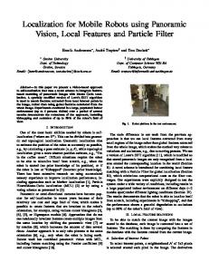
(c1) (c2) Fig. 2 The global localization results of standard MCL ((a1), (a2)), ClusterMCL ((b1), (b2)) and ADC-MCL ((c1), (c2)).
The experiment results of these algorithms are shown in Figure 2. The robot’s real position is marked by a small hollow square. The short green line indicates the orientation of the robot, and the two longer blue lines plot out the robot’s field of view. Figure 2(a1) and (a2) show the localization results of standard MCL, where the tiny grey dots show the distribution of the particles. It is clear that standard MCL failed in this case, since all of the particles have converged to the position which is nearly symmetric to the robot’s real position in (a2). In contrast to standard MCL, both Cluster-MCL and our ADC-MCL successfully kept track of the robot’s real pose, with the results shown in (b1), (b2) and (c1), (c2) respectively. The groups of particles with different colour correspond to the different clusters in these two algorithms. Table III shows the result of 100 independent runs of these three algorithms. Though in ideal cases the standard
B. In Symmetric Indoor Environment In this scenario, we focus on the comparison between ADC-MCL and Cluster-MCL. The environment is shown in Figure 4. It is a 20m × 30m symmetric indoor environment. Initially, the robot is located in one of the rooms, and during the localization process it will move to another room. The trajectory of the robot is shown by the red dotted line. door wall Start point
End point
Fig. 4 The symmetric indoor environment.
Figure 5 shows the localization results of Cluster-MCL algorithm. After a few steps, the particles converged to two distinct hypothetical positions with two clusters formed accordingly (Fig. 5(a)). As the robot moves, the particles in both clusters diffuse. Then, as shown in Fig. 5(c), the door of the target room is detected. However, because the doors of the two neighbouring rooms look almost the same, the particles in each cluster will actually assemble around two similar positions. But, unfortunately, due to the fact the
1063
diversity of the particles in the same cluster can’t be well kept by Cluster-MCL, only one hypothesis survived for each cluster in Fig. 5(d). This leads to the failure of Cluster-MCL. Our ADC-MCL overcomes the drawbacks of ClusterMCL mentioned above. The result is shown in Figure 6. The situations described by Figure 6(a) and (b) are similar to those of Cluster-MCL. But, as indicated by Figure 6(c), when the door of the target room is detected, the particles in each cluster are partitioned into two different clusters. That is, the previously formed two clusters split into four descendant clusters. Seen from Figure 6(d), the robot’s true pose is correctly tracked till the end of the test. Table IV shows the comparison result of 100 independent runs of Cluster-MCL and ADC-MCL, which indicates that ADC-MCL is more robust and effective.
(a)
their spatial similarity, and all these clusters are dynamically evolved by merging the overlapping ones and splitting those become too diffuse or the particles in them gather to some sub-clusters inside. An attractive feature of this method is that one cluster usually corresponds to one distinct mode of the multimodal target distribution. This inspires the method for adapting the sample size of each cluster to its underlying state uncertainties, in order to promote computational efficiency without sacrificing estimation accuracy. The theoretical lower bound of particle number for any cluster is derived, based on the central limit theorem in multidimensional space and the statistic theory of Importance Sampling (IS). In addition, the method for robustly tuning the sample size of each cluster to satisfy the derived lower bound is proposed. The effectiveness of our ADC-MCL has been shown by simulation, where it can keep track of the robot’s real pose throughout the experiments in symmetrical environments. Both the number of clusters and particles are adaptively tuned according to the property of the posterior distribution, which leads to significant improvement in both robustness and computational efficiency. ACKNOWLEDGMENT
(b)
This work is supported by the National Natural Science Foundation of China under Grant NO. 60674017 and the Education Foundation of Tsinghua University with Grant NO. 202025001. REFERENCES
(c) (d) Fig. 5 Global localization using Cluster-MCL.
(a)
(b)
(c) (d) Fig. 6 Global localization using ADC-MCL. TABLE IV RESULT OF 100 INDEPENDENT RUNS OF CLUSTER-MCL AND ADC-MCL
Cluster-MCL ADC-MCL
Times failed 32 0 IV. CONCLUSION
An adaptive dynamic clustered particle filtering method for mobile robot global localization is proposed. First, the particles are classified into a number of clusters based on
[1] P. Jensfelt, S. Kristensen, Active Global Localisation for a Mobile Robot Using Multiple Hypothesis Tracking, IEEE Transactions on Robotics and Automation, 17 (5) (2001) 748 -760. [2] K. Arras, J.A. Castellanos, R. Siegwart, Feature-based multi-hypothesis localization and tracking for mobile robots using geometric constraints, In: Proceedings of IEEE International Conference on Robotics and Automation, 2002, pp. 1371–1377. [3] W. Burgard, D. Fox, D. Henning, T. Schmidt, Estimating the absolute position of a mobile robot using position probability grids, In: Proceedings of the National Conference on Artificial Intelligence (AAAI-96), 1996, pp. 896–901. [4] D. Fox, W. Burgard, S. Thrun, Markov localization for mobile robots in dynamic environments, Journal of Artificial Intelligence Research, 11 (1999) 391–427 [5] P. Jensfelt, O. Wijk, D.J. Austin, M. Andersson, Experiments on augmenting condensation for mobile robot localization, In: Proceedings of the International Conference on Robotics and Automation, 2000, pp. 2518–2524. [6] D. Fox, W. Burgard, F. Dellaert, Monte Carlo Localization: Efficient Position Estimation for Mobile Robots, In: Proceedings of the 16th National Conf on Artificial Intelligence (AAAI-99), 1999, pp. 343-349. [7] S. Thrun, D. Fox, W. Burgard, et al., Robust Monte Carlo Localization for Mobile Robots, Artificial Intelligence, 128 (1) (2001) 99-141. [8] D. Fox, Adapting the sample size in particle filters through KLDsampling, International Journal of Robotics Research, 22 (12) (2003) 985–1003. [9] A. Soto, Self Adaptive Particle Filter, In: Proceedings of International Joint Conferences on Artificial Intelligence (IJCAI-05), 2005, pp. 1398–1406. [10]C. Stachniss, G. Grisetti, W. Burgard, Recovering particle diversity in a Rao-Blackwellized particle filter for SLAM after actively closing loops, In: Proceedings of the IEEE International Conference on Robotics and Automation, 2005, pp. 667–672. [11]A. Milstein, J.N. Sanchez, E.T. Williamson, Robust Global Localization Using Clustered Particle Filtering, In: Proceedings of 18th National Conference on Artificial Intelligence AAAI-02, 2002, pp. 581–586. [12]J.S. Liu, R. Chen, Blind Deconvolution via Sequential Imputations, Journal of the American Statistical Association, 90 (430) (1995) 567– 576. [13]A. Doucet, et al., On sequential Monte Carlo sampling methods for Bayesian filtering, Statistics and Computing, 10 (3) (2000) 197–208. [14]J. Geweke, Bayesian Inference in Econometric Models using Monte Carlo Integration, Econometrica, 57 (6) (1989) 1317–1339.
1064