Permutation Filters: A Class of Non{Linear Filters Based ... - CiteSeerX

Permutation Filters: A Class of Non{Linear Filters Based on Set Permutations 1 Kenneth E. Barner and Gonzalo R. Arce Department of Electrical Engineering University of Delaware Newark, Delaware 19716 (302) 451{8030 Abstract In this paper we introduce and analyze a new class of non{linear lters which have their roots in permutation theory. We show that a large body of non{linear lters proposed to date constitute a proper subset of Permutation Filters (P Filters). In particular, rank{order lters, weighted rank{order lters, and stack lters embody limited permutation transformations of a set. Indeed, by using the full potential of a permutation group transformation we can design very ecient estimation algorithms. Permutation groups inherently utilize both rank{order and temporal{order information; thus, the estimation of non{stationary processes in Gaussian/non{Gaussian environments with frequency selection can be eectively addressed. An adaptive design algorithm which minimizes the mean absolute error criterion is described as well as a more exible adaptive algorithm which attains the optimal permutation lter under a deterministic least normed error criterion. Simulation results are presented to illustrate the performance of permutation lters in comparison with other widely used lters.

ASSP EDICS 4.2.5 Submitted to the IEEE Transactions on Signal Processing. Permission to publish this abstract separately is granted.

This research was supported in part by the DuPont Teaching Fellowship, and by the National Science Foundation under the grant MIP{9020667 1

List of Figures 1 2 3 4 5

6

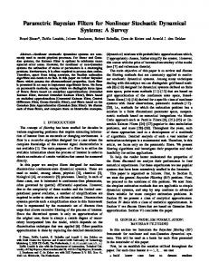
Desired multi{tone non{stationary signal. : : : : : : : : : : : : : : : : : : : : : : Filter learning curves for the case with tone interference and (0:05; 2:0; 15:0) distributed additive contaminated Gaussian noise. (The L1 norm was used for the LNE optimizations.) : : : : : : : : : : : : : : : : : : : : : : : : : : : : : : : : : : Power spectral density of the desired multi{tone non{stationary signal. : : : : : : Observed and lter estimate signals for the case with tone interference and (0:05, 2:0; 15:0) distributed additive contaminated Gaussian noise: (a) observed, (b) linear FIR, (c) combination, (d) stack, (e) permutation, (f) reduced set permutation. : : Power spectral densities of the observed and lter estimate signals for the case with tone interference and (0:05; 2:0; 15:0) distributed additive contaminated Gaussian noise: (a) observed, (b) linear FIR, (c) combination, (d) stack, (e) permutation, (f) reduced set permutation. : : : : : : : : : : : : : : : : : : : : : : : : : : : : : : : : Top: Video sequence estimate errors for 3  3 window permutation and stack lters. The lters were trained two ways, using all 120 frames, and only the rst frame. Bottom: The dierences between estimate errors based on training the lters with all 120 frames and only the rst. : : : : : : : : : : : : : : : : : : : : : : : : : : :

i

24 27 28 30

33

36

List of Tables 1 2

3 4

Recursive least L normed errors training algorithm. : : : : : : : : : : : : : : : : The output distributions for permutation lters operating on i.i.d. input variables with common distribution (
). The output distribution is given as a polynomial of  for all possible values of K1 ; K2, and K3 . The number of unique lters for each set of K1; K2, and K3 values as listed as K , and the output mean and variance are given for zero mean unit variance bi{exponentially distributed input samples. : : : MAE values for the estimates of the non-stationary two tone desired signal based on a noisy observation. The observation is the desired signal with tone interference and additive contaminated Gaussian noise. : : : : : : : : : : : : : : : : : : : : : : MSE values for the estimates of the non-stationary two tone desired signal based on a noisy observation. The observation is the desired signal with tone interference and additive contaminated Gaussian noise. : : : : : : : : : : : : : : : : : : : : : :

ii

17

22 25 26

1 Introduction Considerable attention has been given in the signal processing literature to the de nition and testing of rank{order lters and their generalizations [2, 7, 13, 16, 22, 25, 28, 29]. These lters have their roots in order statistics, which provides a mechanism that attains advantages over traditional linear lters; they can be designed (a) to be robust in environments where the assumed statistics deviate from Gaussian models and are possibly contaminated with outliers, and (b) to track signal discontinuities without introducing transient or blurring artifacts as linear lters do. Notably, the ordering of observation samples provides signi cant information from which robust estimates can be construed [11]. If x = (x1; x2; : : : ; xn) is the observation vector, rank{order lters rely on the sorting of x where x(i) is the i'th largest sample in x, and where xr is the sorted vector xr = (x(1); x(2); : : :; x(n)): The median lter is perhaps the most widely used rank{order lter whose output, at each time interval, is the sample median of the observation vector. To generalize median and rank{order lter, order statistic lters, or L lters, were introduced [7]. L lters take as their output a linear combination of the samples in the sorted vector xr , rather than simply a single order statistic. Nevertheless, rank order information alone is not sucient in many important applications. Order statistic based estimators suer from a fundamental limitation that is best explained by way of an example. Consider the vectors x1 = (10; 4; 7; ?10; ?1; 8; 8, ?1; ?10; ?7; 4) and x2 = (10; 8; 8; 4; 4; ?1; ?1; ?7; ?7; ?10; ?10), which are observations of a sampled sinusoid and decreasing monotonic sequence respectively. Although these vectors have very distinct and dierent patterns, their corresponding sorted vectors are identical: xr = (?10; ?10; ?7; ?7; ?1; ?1; 4; 4; 8; 8; 10). In fact, the above sorted vector could have been produced by over 39 million dierent permutations of x1. Clearly, order statistics based lters fail to exploit the temporal context of a sequence. Many generalizations of rank{order lters have been proposed that incorporate some form of temporal information [9, 13, 28]. Among these are stack lters, which constitute a large class of lters that embody many well known lters such as rank{order lters, weighted rank{order lters, multistage rank{order lters, some composition of discrete morphological operators, and many other estimators that have been successfully used in several applications. As we will show in this paper, stack lters partially overcome the shortcomings of order statistic based lters; nevertheless, due to their constrained structure they can exhibit poor performance [6]. The limitations of order statistic type lters have also been addressed through the development of combination, or C lters [13], which are referred to as Ll lters in [24]. These methods combine the ideas of linear and L lters, assigning the output to be a weighted sum of the input samples where the weights are a function of both sample rank and temporal position. These methods 1

are ecient in non{Gaussian environments and in dealing with outliers. However, due to their weighted sum approach, combination lters still suer from poor performance in non{stationary applications where signal discontinuities are common. Performance improvements can be gained in combination type lters by selecting sample weights according the temporal{order/rank{order relationship between multiple samples. This concept has been formulated as a permutation lattice [19], which progressively covers lters from the simple linear lter to the complex generalized combination (N !{Ll) lter [13, 24]. In this paper we introduce and analyze Permutation lters, or P lters. This is a new class of non{linear lters that has its roots in permutation theory. The lter de nition follows from the fact that the mapping from the temporally ordered vector x, to the rank ordered vector xr de nes a permutation of the elements comprising x. This permutation inherently incorporates both rank{order and temporal{order information. A permutation lter associates with each such permutation a speci c order statistic. The output of a permutation lter operating on a vector x is then de ned to be the order statistic associated with the mapping x 7! xr. Also de ned in this paper is the Reduced set Permutation lter, or RP lter. The reduced set permutation lter has the same general structure as permutation lters. These lters, however, consider several permutations to be isomorphic, thus reducing the cardinality of the class. We show that a large body of non{linear ltering methods proposed to date, such as rank{ order, weighted rank{order, and stack lters, embody limited permutation transformations of a set. Indeed, by using the full potential of a permutation group transformation we can design very ecient estimation algorithms. By operating on both rank{order and temporal{order information, permutation and reduced set permutation lters can be eectively applied to the estimation of non{stationary processes in Gaussian/non{Gaussian environments with frequency selection. It should be noted that other ltering techniques have been proposed that are also rooted in permutation theory. Speci cally, generalized combination and N !-Ll lters [13, 24], and more recently, permutation lter lattices [19], are based on permutation theory. These lters, however, form weighted sum estimates. In a permutation lter, the output is restrict to be one of the input samples. As a consequence, permutation lters are a subset of the larger classes of generalized combination, N !-Ll, and (the highest level) permutation lattice lters, which are all equivalent. Although in many signal processing applications linear combinations of samples lead to highly eective lter structures, there are important applications where the averaging eects of linear combinations are not desirable. For instance, in processing signals such as images with non{stationary mean values, averaging eects lead to unacceptable blurring. By restricting the output to be one of the input samples, permutation lters can be designed to accurately track discontinuities and minimize the eect of outliers within the observation window. Moreover, per2

mutation lters can be used on any signal which has at least two natural orderings, in the case examined here, temporal and rank2, even if linear combinations are not possible due to the nature of the signal3. The paper is organized as follows. In Section 2, we introduce some basic concepts of group theory as they apply to signal estimation. In this section we also de ne the permutation and reduced set permutation lters, as well as describe some of their cardinality properties. The relationship between stack and permutation lters is also addressed in Section 2. In Section 3, we consider the optimal ltering problem where we develop adaptive algorithms to minimize the mean absolute error (MAE) and the sum of least norm errors (LNE) criteria. While the former is inherently statistical, the later is deterministic. In Section 4, we derive the statistical properties of permutation lters, primarily the output distributions and related characteristics. Computer simulations are presented in Section 5, which illustrate the performance of permutation lters. These results are compared with that of other widely used lters. We conclude with Section 6, by providing some comments and indicating directions for future work.

2 Permutation Filters A permutation of a set is a one{to{one mapping of onto . A permutation group is an ordered pair ( ; S ), where is a set and S is a group of permutations on . The degree of ( ; S ) is o( ), and de ned as the number of elements, or points, in . The image of a point  2 under a permutation p 2 S is denoted p. The unique inverse of the permutation p, written p?1, is de ned by pp?1 = I , where I is the identity permutation that leaves all points xed. Thus if p takes  to p, then p?1 takes p to . Let ( ; S ) be a permutation group of nite degree, and let p 2 S . Then p can be speci ed in two{row form by listing each point in with the corresponding image under p below. To illustrate, de ne N to be the set of natural numbers f1; 2; : : :; N g, and SN to be the set of all permutation of N points. Then for p 2 SN , the two{row form of p is ! ! 1 2


N  p = 1p 2p


Np = p ; (1) where  2 N . The unique inverse p?1, can also be expressed in two{row form by listing each Other possible orderings include temporal and likelihood. For example, linear combinations can not be taken of the musical notes A,B, : : :, G. Notes of a song do have two natural orderings, temporal and likelihood, which can be related by a permutation. A song can be ltered by relating a speci c input note with each mapping (permutation) from temporal ordering to likelihood ordering. 2 3

3

point below it's image under p,

! ! 1 p 2 p


Np p = 1 2


N =  : (2) In the remainder of this paper we concentrate on the set of natural numbers N , and the group of permutations SN . The group SN is known as the symmetric group, and has o(SN ) = N !. In the following development the permutations in SN are used to relate the temporal{order and rank{order of samples in an observation window. p?1

2.1 Permutation Filter De nition

In the context of discrete{time signal estimation, consider a sequence fxg and de ne the N = 2K + 1 element observation vector x(n) 2 RN as

x(n)

= (x(n ? K ); x(n ? K + 1); : : : ; x(n); : : :; x(n + K )) = (x1(n); x2(n); : : : ; xN (n));

(3) (4)

where xi(n) = x (n + i ? (K + 1)). Thus x(n) is a temporally{ordered observation vector centered at x(n). The observation samples can also be ordered by rank. De ne xr (n) to be the vector containing the rank{ordered observation samples,

xr(n) = (x(1)(n); x(2)(n); : : :; x(N )(n));

(5)

where x(1)(n)  x(2)(n) 


 x(N )(n). From the temporally{ and rank{ordered observation vectors x(n) and xr(n), we would like to produce an estimate d^(n) of some desired process d(n). Clearly, by shifting the observation window we sequentially produce the estimates d^(n), d^(n + 1), d^(n + 2), and so on. Since the index n is by default the index of the estimate's location, for the sake of notational simplicity, we can drop the index n and concentrate on the estimate produced at a given location. Thus when there can be no confusion, the temporal{order and rank{order observation vectors are expressed as x = (x1; x2; : : : ; xN ) and xr = (x(1); x(2); : : :; x(N )): Since each point in N is used to index samples in both x and xr, the mapping from the temporal{order indices to the rank{order indices de nes a permutation. In general, the mapping of indices by a permutation p 2 SN is expressed as

xp = (x1p; x2p; : : : ; xNp):

(6)

The observation permutation, denoted as px , is de ned as the permutation that maps x to xr ,

xpx = (x1px ; x2px ; : : : ; xNpx ) = (x(1); x(2); : : :; x(N )) = xr: 4

(7)

This de nition establishes the equivalences xi  x(ipx) and xip?x  x(i). To guarantee that the observation permutation is well de ned (one{to{one), stable sorting is performed when x has constant subsequences. That is, the original ordering is retained within each subsequence. Also, for a stochastic sequence fxg, each px 2 SN can have a non{zero probability of occurrence. 1

Example 2.1: Suppose the 5 element temporally{ordered observation is x = (3; 5; ?1; 0; 4). The corresponding rank{ordered observation is xr = (?1; 0; 3; 4; 5), and the observation permutation is ! 1 2 3 4 5 px = 3 5 1 2 4 : (8)

2

The class of permutation lters, which is de ned below, consists of lters that output a ranked sample from xr for each observation x. The speci c ranked sample taken as the output is a function of the observation permutation. Thus both rank and temporal information4 is incorporated in the ltering process. Since many observation permutations will have properties that are in some way similar, or related, such permutations will produce a common output. We therefore partition the group of permutations into N sets called blocks, placing all permutations that produce a common output in a single block. De nition 2.1: Let H = fH1 ; H2 ; : : : ; HN g be a set whose elements are possibly empty subsets of SN . If the elements of H are pairwise disjoint and their union is SN , then H is called a partition of SN , and the elements of H are called blocks of the partition H. The set of all such partitions is written H. 2

De nition 2.2 Permutation Filters: For a partition H 2 H , let `x be the index of the block that contains the observation permutation px , i.e., px 2 H`x . Then the permutation lter FP (x; H) is de ned as FP (x; H) = x(`x): (9)

2

The permutation ltering operation is thus a function of the partition H 2 H. The permutations contained in the block Hi are, by de nition, associated with an output x(i). Consequently, by changing the partition H, permutation lters can be designed to perform a large number of ltering operations. Possible lters range from simple rank{order operators, to very ecient application speci c estimators. It should be understood that the permutation contains temporal and rank information for time sequence signals, and temporal and spatial information for signals such as images. Also, other natural orderings, such as temporal and likelihood, can be related in this fashion and be the basis for selecting an output sample. 4

5

Example 2.2: Suppose the group of permutations is partitioned as follows: Hl = SN ; Hi = f;g, i 6= l. Then, since px 2 Hl 8x 2 RN , FP (x; H) is the rank{order lter that always outputs the l'th ranked input sample. If l = (N + 1)=2, then FP (x; H) is the window size N median lter. 2

Before relating permutation lters to other ltering techniques, we derive the cardinality of the permutation lter class. First, it is show that each partition H 2 H de nes a unique permutation lter. This result is then used to determine the size of the class of permutation lters. Theorem 2.1: Each partition H 2 H de nes a unique permutation lter, and the number of unique window size N permutation lters is N N !. Proof: To show uniqueness assume H = fH1 ; H2 ; : : :; HN g and H0 = fH10 ; H20 ; : : : ; HN0 g are such that H; H0 2 H, H 6= H0, and FP (x; H) = FP (x; H0) 8 x 2 RN . Then there exists p 2 SN such that p 2 Hi and p 2 Hj0 , where i 6= j . Take xr = (1; 2; : : : ; N ). Then for x = xrp?1 , the observation permutation px = p and FP (x; H) = x(`x ) = i 6= j = x(`0x) = FP (x; H0), which is a contradiction. Thus each partition H 2 H de nes a unique permutation lter, and the number of unique lters is o( H ). Since each element of H is a N block partition of SN , o( H) = N o(SN ) = N N !. 2

2.2 Relating Permutation, Weighted Rank{Order and Stack Filters As can be seen from Example 2.2, the set of rank order lters is equivalent to a trivial singleton partition. A more interesting and larger class of lters is the weighted rank order lters, which replicate a xed amount of times samples in the observation window [9, 17, 31]. The resultant expanded set that is then ranked, and the appropriate rank element is taken as the output. By varying the representation of the input samples in the expanded set, weighted rank order lters emphasize certain spatial locations while de-emphasizing others. The number of times each sample is replicated in a weighted rank order lter is determined by the weight vector w = (w1; w2; : : :; wN ): The weighted rank order lter Rl (w  x) is de ned by

Rl(w  x) = l'th largest (w1  x1; w2  x2; : : :; wN  xN ) (10) wi times z where wi  xi is the replication operator wi  xi = xi; xi;}|: : :; x{i A special case of weighted rank order lters is the center weighted median. Center weighted median lters have weighting vectors w = (1; : : : ; 1; w; 1; : : : ; 1), where  = N2+1 . It has been shown in [21] that the center weighted median is equivalent to a multi{stage median lter, where the output is the median of three elements, the center sample and two (symmetric) order statistics. The next theorem rst extends the results in [21] to include all weighted rank order lters in which 6

only a single element, designated as x , may have weight w greater than one. We shall refer to these lters as simply weighted rank order lters. Next, the result is used to construct a non{trivial partition of SN such that the resulting permutation lter is equivalent to the simply weighted rank order lter. Theorem 2.2: The following window size N ltering operations are equivalent.

1. Rl(w  x) where w is a simple weighting vector with w  1 and wi = 1 for i = 1; 2; : : : ; N , i 6= . 2. R2(x(l ); x ; x(l )) where l1 = max(l + 1 ? w ; 1), and l2 = min(l; N ). 1

2

3. FP (x; H) where H 2 H is de ned by partitioning the permutations p 2 SN as follows: 8 fp : p  l g for i = l > > < fp : p  l12g for i = l12 (11) Hi = fp : p = ig for l < i < l 1 2 > : f;g for 1  i < l1 and l2 < i  N Proof: See [4]. 2 The next example illustrates the partitioning of SN such that the permutation lter is identical to a simply weighted rank order lter. Example 2.3: Consider the simply weighted rank order lter R2 (w  x) where w = (1; 2; 1). The equivalent multi{stage median lter is R2(x(1); x2; x(2)), since l1 = max(l + 1 ? w; 1) = max(2 + 1 ? 2; 1) = 1 and l2 = min(l; N ) = min(2; 3) = 2. Also, o(S3) = 6 and is comprised of the elements ! ! 1 2 3 1 2 3 p1 = 1 2 3 p2 = 1 3 2 ; (12) ! ! 1 2 3 1 2 3 p3 = 2 1 3 p4 = 2 3 1 ; (13) ! ! 1 2 3 1 2 3 p5 = 3 1 2 p6 = 3 2 1 : (14)

By partitioning S3 into the three blocks H1 = fp3; p5g; H2 = fp1; p2 ; p4; p6g, and H3 = f;g according to Theorem 2.2, the permutation lter de ned by H = fH1; H2; H3g is such that FP (x; H) = R2(x(1); x1; x(2)) = R2(w  x). The partition of S3 shows that the maximum observation sample is never taken as the output since H3 = f;g. Also, four of the six possible observation permutations yield the sample median as the output, while two observation permutations produce an output that is the minimum sample. 2 7

As Theorem 2.2 shows, and Example 2.3 illustrates, simply weighted rank order lters can be expressed as permutation lters. The allowable partitions of SN in the permutation lter implementation, however, constitute a very small subset of total number of possible partitions. A larger class of lters, which include all weighted rank order lters as a subset, are stack lters [10, 28]. We will now show that stack lters are a proper subset of permutation lters. Also, for an arbitrary stack lter we give the partition H 2 H that will result in an equivalent permutation lter. Stack lters are a large class of non{linear lters based on the set of positive Boolean functions [28]. A Boolean function is positive if and only if in reduced form it contains no complemented elements [12]. Thus, any stack lter can be expressed in a sum of products form which contains no complemented elements [28]. For a stack lter FS (
), operating on an observation x, the sum of products representation can be expressed as

FS (x) = 1 + 2 +


+ k ;

(15)

where each i is a product of terms i = xi xi


xiki : In the above expression each of the k product terms has two interpretations depending on the domain of the observation x. If x is binary, as in a threshold decomposition architecture, then i is the Boolean AND product of xi ; xi ; : : : ; xiki . If x is multi{level, then i is understood to be the minimum operator, i = min(xi ; xi ; : : : ; xiki ). Similarly, the addition operator is understood to be a Boolean OR in the binary domain and the maximum function for multi{level samples. Thus the stack lter in (15) can be expressed as  n oki k FS (x) = max min xij j=1 : (16) 1

2

2

1

1

2

i=1

We now prove a theorem that gives the partition H of SN which results in a permutation lter that is equivalent to an arbitrary stack lter. In this theorem we use the set subtraction operator n, which is de ned by A n B = f 2 A :  2= B g. Theorem 2.3: A window size N stack lter de ned by the Boolean expression F (x) = Pk ki x S

i=1 j =1 ij

is equivalent to the permutation lter FP (x; H), where H 2 H is uniquely de ned by partitioning the permutations p 2 SN as follows: 11 1 0N ?1 ki 00 ki [ [ [k @@ [ fp : ij p = mgAA (17) fp : ij p = N gA n @ HN = i=1

Hl =

00 k i [k @@ [

i=1

j =1

m=1 j =1

j =1

1 0 l?1 k 11 N i [ [ [ fp : ij p = lgA n @ fp : ij p = mgAA n Hn m=1 j =1

8

n=l+1

(18)

for l = N ? 1; N ? 2; : : : ; 2, and

H1 =

ki [k [ i=1 j =1

fp : ij p = lg n

N [ n=l+1

Hn

(19)

Proof: See [4]. 2 Before leaving this section we give an example of a permutation lter that is not a stack lter. Thus showing stack lters are a proper subset of permutation lters. Example 2.4: Consider the window size 3 permutation lter de ned by the partition H = ffp2 ; p4g; fp1 ; p6g; fp3; p5gg, where again p1; p2; p3; p4 ; p5 are the elements of S3 enumerated in Example 2.3. The permutation lter de ned by the disjoint partition H outputs the median ranked sample when this sample occupies the center spatial location in the observation window. Thus like the median lter, FP (x; H) preserves increasing and strictly decreasing sequences, that is they are roots of the lter. Unlike the median lter, FP (x; H) takes the minimum (maximum) rank sample as the output when the maximum (minimum) rank sample resides in the center of the observation window. It is easy to show that there is no stack lter which performs the equivalent ltering operation. If there was an equivalent stack lter, for binary data we would have FS (1; 1; 0) = 0 and FS (1; 0; 0) = 1, which is a violation of the stacking constraint. 2

2.3 Reduced Set Permutation Filters As Theorem 2.1 shows, the number of possible permutation lters grows very rapidly with the window size, even when compared to the number of possible stack lters, which is at least 22N= [10]. With such a large class of lters it is often of interest to, in some logical manner, reduce the number of possible lters. The reduction of the class of permutation lters is the topic of several sequels to this paper [3, 5, 14]. For completeness, we include here a brief discussion of one set of methods used in reducing the class [5]. The other methods are based on extending WOS lters [3] and LUM lters [14, 15] to inclued temporal and rank order information. There are two approaches that can be taken in reducing the number of permutation lters. The rst is to reduce the number of blocks in the partition. This is useful in applications where the lter output need not range over the full set of ranked samples. For example, in noisy environments it may not be desirable to allow the lter output to be either the minimum and maximum samples. In this case the case SN would be partitioned by a N ? 2 block partition, reducing the number of possible partitions to o( H ) = (N ? 2)o(SN ). The second approach, which we shall brie y discuss, reduces the number of possible lters by considering certain observation permutations equivalent. For example, it seems reasonable to consider the observations x = (3; 5; 2; 7; 8; 1; 4; 6; 9) and x0 = 2

9

(2; 5; 3; 8; 7; 1; 4; 6; 9) to have equivalent permutations since they dier by only the transposition of the samples 2 and 3, and 7 and 8. To consider certain permutations equivalent, we must rst recast the group of permutation mappings from N to N . We thus de ne a new set of mappings from N to a set A of \colors", where each mapping from N to A will be called a \coloring" of N . A Reduced set Permutation (RP ) lter is then de ned by associated with each possible coloring a speci c rank element output. These concepts are made precise by the following de nitions. De nition 2.3: Let A = fa1 ; a2; : : :; aM g, M  N , be an set whose element are called colors. Associated with each color ai 2 A is a positive integer valued elements bi, called the color count, such that PMi=1 bi = N . A coloring of N is an assignment of some color in A to each point of N , with the restriction that bi points in N are mapped to color ai. The set of all such colorings is written C ( N ; A). 2 De nition 2.4: For a N element observation x, the observation coloring is written as cx , and de ned by the mapping icx = aj where x(bj )  xi  x(bj?1+bj ) (20) for i = 1; 2; : : : ; N , and where b1 = 1 and bj = bj?1 + bj?1 for j = 2; 3; : : : ; M . 2

The set of colorings C ( N ; A) and the observation coloring cx have de nitions that are similar to the symmetric group SN and the observation permutation px . In fact, if M = N and ai = i, then the de nitions are identical. The number of possible colorings is o (C ( N ; A)) = b !b N!


! bM ! . Thus by taking M < N , the number of coloring can be reduced to levels signi cantly below o(SN ). 1

2

Example 2.5: Take N = 9, M = 3, and b1 = b2 = b3 = 3. Then the number of possible colorings is 9! = 1680, which is signi cantly less than o(S ) = 362880. Let the set of colors o (C ( 9; A)) = 3!3!3! 9 be A = fL; M; U g, where L, M , and U stand for lower, middle, and upper. The observation coloring is now given by the mapping 8 > < L if x(1)  xi  x(3) icx = > M if x(4)  xi  x(6) (21) : U if x(7)  xi  x(9) for i = 1; 2; : : : ; N . Thus i is mapped to L, M , or U if xi is in the lower, middle, or upper third of the ranked set xr . As an example of this mapping consider the two observations x = (3; 5; 2; 7; 8; 1; 4; 6; 9) and x0 = (2; 5; 3; 8; 7; 1; 4; 6; 9). These two observations both correspond to a single observation coloring, which can be written in two{row format as: ! ! 1 2 3 4 5 6 7 8 9 1 2


9 (22) 1cx 2cx


9cx = L M L U U L M M U

10

=

! 1 2


9 : 1cx0 2cx0


9cx0

(23)

2

This example shows how several observations can correspond to the same observation coloring. In fact for an observation x, all vectors obtained by permuting the samples in x which are mapped to the same color correspond to a single observation coloring. Reduced set permutation lters can now be de ned in an analogous manner to permutation lters. De nition 2.5 Reduced Set Permutation Filters: For a partition H 2 H, where H is now the set of all N block partitions of C ( N ; A), let `x be the index of the block that contains the observation coloring cx, i.e., cx 2 H`x . Then the reduced set permutation lter FRP (x; H) is de ned as FRP (x; H) = x(`x ): (24)

2

While the number of RP lters can be designed to be signi cantly less than the number of permutation lters, their performance is often comparable. In Section 5 the performance of the RP lter based on the three colors in Example 2.5 (L; M; U ) is compared to that of a permutation lter and other ltering techniques through computer simulations. The simulations show that the performance of this RP lter is similar to that of the permutation lter, and better than that of the other ltering techniques. Moreover, reduced set permutation lters are a exible class of lters. They oer a method to balance performance, which can (in general) be improved by increasing the number of colors, and complexity, which can be reduced by reducing the number of colors.

3 MAE and Least Norm Error Optimization Two dierent adaptive optimization procedures are discussed in this section. The rst is a modi cation of a method developed for the optimization of stack lters [23]. This method is probabilistic and determines the lter that is optimal under the Mean Absolute Error (MAE) criteria. The second method is a new deterministic procedure that, for a given set of training data, minimizes the sum of L normed errors between the lter estimate and desired signal. This method produces the globally optimal lter, for the given set of training data, under the Least Normed Error (LNE) criteria. The goal of the optimization is to determine the partition H 2 H that de nes a lter that is optimal under the MAE or LNE criteria. Recall that H represents all the possible partition of 11

either the group of permutations SN , or the set of colorings C ( N ; A), depending on the class of lters to be optimized over. In order to implement either the MAE or LNE optimization methods, the elements of SN and C ( N ; A) must be enumerated in some logical manner. This enumeration, or orderly listing, of permutations and colorings is addressed next. Following the enumeration, the MAE and LNE optimization methods are developed.

3.1 Orderly Listing of Permutations and Colorings Through an orderly listing it is possible to obtain the i'th permutation or coloring directly from the number i, and conversely, given a permutation or coloring, it is possible to determine its index without generating any of the other permutations or colorings. The permutations comprising SN can be enumerated as p1; p2 ; : : :; pN ! since jSN j = N !. Also, the integers 1 to N ! can be expressed as

1(N ? 1)! + 2(N ? 2)! +


+ N ?11! + 1; (25) where 0  j  N ? j for j = 1; 2; : : : ; N ? 1 [8]. The index i of a permutation pi can thus be expressed as i = 1+ PjN=1?1 j (N ? j )!. There are many ways to assign the coecients 1; 2; : : : ; N ?1, such that there is a one{to{one correspondence between the coecients and the permutation pi . One simple method is to assign j to be the number of terms (j + 1)pi ; (j + 2)pi ; : : :; Npi that are less than jpi [8]. The factorial expansion coecients are thus de ned to be N X I (kpi < jpi ); (26) j = k=j +1

for j = 1; 2; : : : ; N ? 1. The function I (
) in (26) is the indicator function, de ned by ( is true : I (event) = 10 ifif event (27) event is false The colorings comprising C ( N ; A) can be enumerated as c1; c2; : : :; cjC( N ;A)j, where the number of colorings is jC ( N ; A)j = N !=b1!b2!


bM !. The indexing of the colorings can be performed in a manner analogous to that of the permutations. To simplify the indexing, let the set of colorings A = (a1; a2; : : : ; aM ) be such that ai = i, i.e., the colors are given a numerical values. Then, for a coloring ci, it can be shown [4] that the appropriate j coecients are given by: N X I (kcx < jcx ): (28) j = B1 j k=j +1 where Bj = Mi=1bj;i!, and bj;i is determined recursively by ( bj;i = bj?b1;i ? 1 ifelsejcx = i ; j ?1;i 12

(29)

for j = 2; 3; : : : ; N ? 1, with initial condition b1;i = bi. This expression for the coloring index coecients diers from that for the permutation index coecients by only the Bj term. In fact when b1 = b2 =


= bN = 1, each Bj = 1 and the two index expressions are equal. This, of course, is no surprise since the set of colorings is equal to the group of permutations when b1 = b2 =


= bN = 1. The orderly listing of elements allows us to de ne the observation permutation and coloring index. This de nition is then used to express a partition H 2 H as a decision vector, which simpli es the necessary optimization notation. De nition 3.1: The permutation (coloring) index of an observation x is the value of i such that pi = px (ci = cx ). 2

A partition H 2 H can now be equivalently expressed as a decision vector, which for a permutation lter, has the form ` = (`1; `2; : : :; `N !); (30) where by de nition pi 2 H`i for i = 1; 2; : : : ; N !. Thus, `i is the rank index of the element taken as the output by FP (x; H) for all observations x with permutation index i, i.e., FP (x; H) = x(`i). This notation also holds for reduced set permutation lters, the only dierence being the number of elements in the decision vector. It will be shown that this decision vector notation simpli es the optimization, since the optimal lter can be found by optimizing each of the terms in ` independently. Example 3.1: To clarify the relationship between a partition and decision vector, consider the case N = 2. In this case, there are two permutations, p1 and p2, and 22! = 4 partitions. The four partitions, and their equivalent decision vector representations are:

H1 H2 H3 H4

H1 p1 p2 p1p2 ; (31) H2 p2 p1 ; p 1 p2 ` (1,2) (2,1) (1,1) (2,2) Examining the four partitions shows that H3, or equivalently ` = (1; 1), de nes a minimum lter, while H4, or equivalently ` = (2; 2), de nes a maximum lter. 2

3.2 Minimum Mean Absolute Error The optimization over the class of permutation and reduced set permutation lters under the MAE criteria will now be addressed. The development presented here assumes the optimization is to be performed over the class of permutation lters. The optimization over the class of reduced 13

set permutation lters follows similarly. In the development below, simply substituting ci for pi , N! b !b !


bM ! for N !, and generating the observation coloring index rather than the permutation index, results in the optimization being performed over the class of reduced set permutation lters. The optimal lter under the MAE criteria minimizes the cost E [jd(n) ? FP (x(n); H)j] ; (32) provided the desired signal d(n) and the observation x(n) are jointly stationary. This expectation can be expanded by conditioning on the observation permutation, N! h i X E jd(n) ? FP (x(n); H)j : px(n) = pi Pr(px(n) = pi) (33) E [jd(n) ? FP (x(n); H)j] = i=1 N! h i X E jd(n) ? x(`i)(n)j : px(n) = pi Pr(px(n) = pi ); (34) = 1

2

i=1

where x(`i)(n) is the rank `i element inh x(n). In this form we see that for i given signal statistics, each of the conditional expectations E jd(n) ? FP (x(n); H)j : px(n) = pi , is a function of a single parameter `i . Moreover, `i aects that conditional expectation exclusively. Thus optimizing the decision vector ` with respect to the MAE in (32), is equivalent to optimizing each term of ` independently with respect to the appropriate conditional MAE in (34). In this manner, a large optimization problem has been broken into many smaller and simpler optimization problems, in which only a single parameter must be determined. Since `i speci es the rank element taken as the output by a permutation lter for all observations with permutation index i, the optimization of this parameter is equivalent to nding the optimal rank order lter to operate on fx(n) : px(n) = pi g. Accordingly, determining the optimal decision vector ` is equivalent to determining the N ! optimal rank order lters to operate on the conditioned data. There are several methods for determining optimal rank order lters. If the signal statistics are known, then the optimal rank order lter can be determined through a linear program [10]. A second more ecient method of determining the optimal lter is through adaptive stack ltering, where the lter is restricted to be a rank order operator. There are currently several adaptive methods for determining the optimal stack lter [20, 23, 32], all of which require training sequences of both the desired and corrupted signals. Furthermore, these methods require that the signals be decomposed through thresholding. Recently, a new optimization method based on the LMS algorithm has been developed for rank order and stack lters [30]. This method does not require thresholding, but produces a suboptimal lter because of a simple linear model used to approximation the unit step function. The adaptive stack ltering methods of optimization are stochastic procedures, converging to the optimal lter probabilistically over time. Next we give a simple deterministic method of optimization which returns the optimal permutation lter for a given training sequence. Moreover, the 14

proposed optimization method operates in the real domain, free from the complexities associated with thresholding of training sequences.

3.3 Least L Norm Error We now derive an iterative method for determining the permutation, or reduced set permutation, lter that minimizes the sum of L normed errors between a desired signal and the lter estimate. As in the previous section, the development assumes the optimization is to be performed over the class of permutation lters. Again, the optimization over the class of reduced set permutation lters follows directly by substituting ci for pi , b !b N!


! bM ! for N !, and generating the observation coloring index rather than the permutation index. Following the development of the optimization under the MAE criteria, the global LNE optimization problem is broken up into N ! smaller optimization problems, each of which is over a single parameter. Unlike the previous case, however, the iterative update is deterministic, not stochastic. After each update the optimal lter, with respect to all samples \seen", is returned. The proposed method also incorporates an exponential \forgetting" factor, making it suitable for use in non{stationary environments. Let fd(n)g and fx(n)g be M sample training sequences representing the desired and corrupted signals respectively. Also, assume end eects have been eliminated from the sequences. That is, the training sequences are such that the lter window does not extend beyond available data samples at either the beginning or end. Take E (M ; H) to be the sum of L normed errors generated by the lter de ned by H, M X (35) E (M ; H) = jd(n) ? FP (x(n); H)j : 1

The partition H

 2 H

2

n=1

is de ned to be that which minimizes the sum of L estimate errors,

E (M ; H)  E (M ; H) 8 H 2 H; H 6= H:

(36)

The permutation lter FP (x(n); H) is then the optimal lter under the least L normed error criteria. If the inequality in (36) is not proper, then a tie braking rule is used to obtain a single partition H. The sum of L normed errors in (35) can be reordered according to the permutation of the observation vectors x(n). Let i1; i2; : : :; iMi be the temporal indices of the observation vectors with permutation index i, i.e., px(in) = pi for n = 1; 2; : : : ; Mi. Then the sum of L normed errors in (35) can be expressed as N! X (37) E (M ; H) = Ei (M ; H); i=1

15

where

Ei (M ; H) =

Mi X n=1

jd(in) ? x(`i)(in)j :

(38)

Since Ei (M ; H) is a function of a single parameter `i , the minimization of each Ei (M ; H) conditional error sum is a necessary and sucient condition for E (M ; H) to be minimized. Consider the optimization of the term `i with respect to Ei (M ; H). Let Ri;k (M ) be the sum of L normed dierence between x(k)(in) and d(in) for n = 1; 2; : : : ; Mi, Mi X (39) Ri;k (M ) = jd(in) ? x(k)(in)j ; n=1

and write Ri(M ) = [Ri;1(M ); Ri;2(M ); : : : ; Ri;N (M )]T : Then the optimal `i with respect to the conditional error Ei (M ; H), denoted `i , is determined by the minimum element in Ri(M ),

`i = l where Ri;l(M ) = min (Ri;1(M ); Ri;2(M ); : : : ; Ri;N (M )):

(40)

For any H 2 H with pi 2 H`i , the conditional sum Ei (M ; H) is minimized. If there is not a unique minimum element in the vector Ri(M ), then in order to force `i to be single valued some tie breaking rule must be employed. For example, a tie between two values satisfying (40) may be broken by accepting the one which speci es an output x(`i )(n) that is closest in rank to the median sample x( N )(n). Alternately, a tie may be broken by taking `i to be the value which satis es (40) and speci es an output x`i p?i (n) which is temporally closest to x(n). The decision vector ` = (`1; `2; : : : ; `N !), determined by (40) for i = 1; 2; : : : ; N !, de nes a single pairwise disjoint partition of SN . Moreover, this partition minimizes each conditional sum Ei (M ; H) for i = 1; 2; : : : ; N !. Thus the partition de ned by ` is H, and FP (x(n); H) is the optimal permutation lter with respect to the L optimality criteria in (36). The optimal lter can be recursively updated as new training samples become available. When the index n is incremented and a new observation vector enters the sliding window, one of the cumulative dierence vectors Ri(n), and the corresponding decision element `i , must be updated. Let P(n) be a vector that contains the L normed dierence between the desired signal d(n), and each rank{ordered observation sample, h i P(n) = jd(n) ? x(1)(n)j ; jd(n) ? x(2)(n)j ; : : : ; jd(n) ? x(N )(n)j T : (41) +1 2

1

Then the cumulative error vector Ri(n) is updated according to Ri(n) = Ri(n ? 1) + P(n); where i is the permutation index of the new observation x(n). During the training process the above update is performed until the end of the training sequence is reached, or such a time that the lter has been determined to be suciently trained. The optimal lter parameters are then determined according to (40). 16

1. Set n = 1, li = N2+1 , and Ri;l(0) = 0, for l = 1; : : : ; N , and i = 1; : : :; N !. 2. Determine the permutation index i for the observation x(n). 3. Update each Rj (n),

(

Rj (n) = RRjj ((nn ?? 1)1) + P(n)

if j = i : else

4. Set `i = l, where Ri;l(n) = min (Ri;1(n); Ri;2(n); : : :; Ri;1(n)). 5. If n = M or lter is suciently trained stop, else increment n and go t o (2). Table 1: Recursive least L normed errors training algorithm. If the lter is to be used in a non{stationary signal environment, the partition H may need to be periodically updated. To account for the changing signal statistics an exponential \forgetting" factor can easily be added to the sum of L normed estimate errors. The sum to be minimized is now M X (42) E (M ; H) = (M ?n)jd(n) ? FP (x(n); H)j ; n=1

where  2 (0; 1] is the \forgetting" factor. The recursive permutation lter training algorithm that minimizes E (M ; H) in (42) is summarized in Table 1. The algorithm initially sets the permutation lter to the median lter, and then updates the decision vector according to each new observation. The initial setting of the lter has no eect on the updates made as new samples enter the window. This setting eects only those permutations that do not occur in the training sequence. The goal is to set the output associated with the permutations not seen in the training sequence to a reasonable value. The lter could, for instance, be set initially to the identity, or any other permutation lter that a priori information may suggest. The advantages of this new algorithm over the adaptive stack ltering approach are three fold: freedom in choosing error norm, ability to operate in non{stationary environments, and the fact that the training process always returns the optimal lter for the training set. In addition, the optimization is performed in the real domain, free from the complexities associated with thresholding real valued signals. 17

4 Filter Statistics and Properties In this section we examine statistical properties of permutation and reduced set permutation lters. Since any reduced set permutation lter can be expressed as a permutation lter, we concentrate here on the larger more general class of permutation lters. First, the output distribution function of an arbitrary permutation lter is determined. Then, under the simplifying assumption of independent and identically distributed (i.i.d.) input samples, several properties of permutation lters are derived. As in the previous sections, we take the input to a permutation lter to be a real valued vector, which we assume to have a continuous density function. Suppose the N element observation vector x has the continuous multi{variate distribution (t1; t2; : : :; tN ), i.e., Z tN Zt Zt


?1 (1; 2; : : : ; N )dN dN ?1


d1: (43) Pr(x1 < t1; x2 < t2; : : :; xN < tN ) = 2

1

?1 ?1

De ne (t) to be the probability distribution of the permutation lter FP (x; H). The distribution (t) can be obtained by conditioning (43) on the possible observation permutations, and then summing over all such possibilities. Thus, (t) = Pr(FP (x; H) < t) N! X Pr(FP (x; H) < t; px = pi) = =

i=1 N! X i=1

(44) (45)

Pr(x(`i ) < t; px = pi );

(46)

where ` = (`1 ; `2; : : :; `N !) is the decision vector corresponding to the partition H. Since each permutation pi maps the spatial indexes to the rank indexes, and its inverse p?i 1 has the opposite eect, the probability that the observation permutation is pi is given by

Pr(px = pi) = Pr(x1p?i < x2p?i <


< xNp?i ) Z1 Z1Z1 Z1 (1; : : :; N )dNp?i


d1p?i :


= ?1    1

?1 1p i

1

1

1

?1 (N ?1)p i

?1 2p i

1

(47) (48)

By adding the condition that the rank `i sample be less that t to (47), we have

Pr(x(`i ) < t; px = pi ) = Pr(x1p?i < x2p?i <


< xNp?i ; x(`i) < t) Zt Zt Zt Zt



=  `i ? p ? ?1  p?  p? i Z 1 i Z 1i (1; : : :; N )dNp?i


d1p?i :


  1

1

1 `i p? i

1

1

2

(N

18

1

?1)p?i 1

1

(

1)

(49)

1

1

1

(50)

The probability distribution function (t) of an arbitrary permutation lter FP (x; H), is found by substituting (50) into (46), Z1 Z1 Zt N! Z t Z t Z t X (1; : : : ; N )dNp?i


d1p?i : (51)





(t) = i=1 ?1 1p?i 1 2p?i 1

(`i?1)p?1 `i p?1 i

i

(N ?1)p?1

1

1

i

While the output distribution yields an elegant expression, in practice it is often dicult to calculate. The expression for the distribution can be simpli ed somewhat if the input samples are taken to be independent. We shall strengthen the independence assumption by considering the samples to also be identically distributed. The assumption that the input samples are i.i.d. greatly simpli es the examination of the statistical properties. Although permutation lters loose some of their advantage in an i.i.d. environment, since all permutations are equally likely, properties derived under this assumption still give valuable insight into the ltering operation. Suppose the samples in the observation window are independent with common distribution R t ( )d . Substituting the common distribution into the (t), where by de nition (t) = ?1 conditional probability in (50) and integrating yields N X 1 j (t)(1 ? (t))N ?j Pr(x(`i ) < t; px = pi ) = (52) j =`i (N ? j )!j ! = N1 ! (`i )(t): (53) The term (l)(t) is the distribution of the rank l sample, and is given by the binomial sum ! N X N j (t) (1 ? (t))N ?j : (54) (l)(t) = j j =l The output distribution (t) obtained by summing (53) over all permutations will be comprised of the scaled distributions (1)(t); (2)(t); : : :; (N )(t). To simplify the resulting expression, de ne Ki to be the number of permutations in SN under which FP (x; H) takes the i'th rank sample as the output, i.e., Ki = PNj=1! I (`j = i). Then the output distribution of a permutation lter operating on i.i.d. input samples is given by N X 1 (55) (t) = N ! Ki (i)(t): i=1 Theorem 4.1: If the input samples to a permutation lter are i.i.d. random variables with common distribution (
), and Ki = KN +1?i for i = 1; 2; : : : ; (N ? 1)=2, then for t1 and t2 such that (t1) = 1 ? (t2); we also have (t1) = 1 ? (t2); where (
) is the permutation lter output distribution.

19

Proof: Using the fact that for i.i.d. samples (i) (t1) = 1 ? (N +1?i) (t2),

N X (t1) = N1 ! Ki(i)(t1) 0i=1N ? 1   X = N1 ! B @ Ki (i)(t1) + (N +1?i)(t1) + K N ( N )(t1)CA i=1 0 N? 1     X = N1 ! B @ Ki 2 ? (N +1?i)(t2) ? (i)(t2) + K N 1 ? ( N )(t2) CA i=1 0 N? 1   X = 1 ? N1 ! B @ Ki (i)(t2) + (N +1?i)(t2) + K N ( N )(t2)CA 2

1

+1 2

2

(56)

+1 2

(57)

1

+1 2

2

+1 2

(58)

1

+1 2

i=1

= 1 ? (t2);

+1 2

(59) (60)

since PNi=1 Ki = N !.

2

Corollary 4.1: Permutation lters de ned by partitions H such that Ki = KN +1?i for i = 1; 2; : : : ; N2?1 , are statistically unbiased in the sense of the median.

Proof: This follows from the preceding theorem by taking (t1 ) = 1=2. 2 Thus for permutation lters in which Ki = KN +1?i , the median of the input is the median of the output; such lters, like median lters and self-dual stack lters [31], behave consistently for asymmetric noise. As with stack lters, the output distribution of a permutation lter can be written as an order N polynomial of the input distribution, (t). Expanding the terms in (55), (t) = PNi=0 Cii(t); where C0 = 0 and PNi=1 Ci = 1 since (+1) = (+1) = 1 and (?1) = (?1) = 0 [31]. Also, for unbiased lters PNi=1 Ci=2i = 1=2 by Corollary 4.1. Expressing the permutation lter output distribution as a polynomial of the input distributions allows the moments of the output to be easily calculated [31]. For a given permutation lter

E fxmg

= =

Z +1

tmd (t) Z +1 iCi ?1 tm(t)i?1(t)dt:

?1 N X i=1

(61) (62)

Example 4.1: Take the input samples to a permutation lter to be zero mean i.i.d. bi-exponentially distributed random variables. The distribution of the input samples is given by (t) = 21 e?(jtj= ); where 2 2 is the variance ( > 0). The m'th output moment is given by 1 i?1  1 i?1 ! Z +1 1 Z0 1 N X m m ( t= ) ( t= ) ( ? t= ) ( ? t= ) m 1 ? 2e dt + 0 t 2 e dt ; (63) E fx g = iCi ?1 t 2 e 2e i=1

20

which can shown to simplify to [4] N X E fxmg = ? mm! Ci i=1

! ! i 1 +X 1 i 2i im k=1 k (?2)k km :

(64)

2

Table 2 lists the output distributions of all the window size 3 permutation lters operating on i.i.d. input samples with common distribution (
). The output distributions are listed by subsets determined by the values of K1; K2, and K3, since all lters in such subsets have a common distribution. The output distributions are expressed as polynomials of the common input distribution (
). Also, the number of lters in each subset, denoted as K , is given as well as the output mean and variance corresponding to the case of zero mean bi-exponentially distributed input samples with variance 1.

5 Computer Simulations In this section we present several computer simulations to demonstrate the advantages of permutation and reduced set permutation lters over other commonly used ltering techniques. Also, the lter design methodologies discussed in Section 3 are compared. We show that in non{stationary non-Gaussian environments, permutation lters can be designed to have desirable time domain and frequency domain characteristics. It is demonstrated that by operating on both temporal and rank information, permutation lters can preserve step edges and selectively retain desired frequency components, while removing outliers and unwanted frequencies components. In addition, an example is presented that shows the permutation lter to be more robust with respect to changing signal (image) statistics than the stack lter. The signal models used in the rst set of simulations were rst detailed in [13], and are comprised of multi-tone non{stationary signals. In the following, these multi-tone non{stationary signals are corrupted by tone interference and additive contaminated Gaussian noise. Estimates of the desired signal based on the corrupted version produced by permutation, reduced set permutation, stack, combination, and linear FIR lters are compared subjectively through a visual examination of the output waveforms, as well as quantitatively by means of the estimate MAE and Mean Squared Error (MSE) values. Also, the power spectral densities (PSD) of the estimates are compared to show the frequency characteristics of each estimate. The reduced set permutation lter used here is that based on the three colors L (Lower), M (Middle) and U (Upper), which was described in Example 2.5. Through a comparison of the estimate outputs it is shown that the linear FIR and combination lters smooth the signal discontinuity edges to a greater extent than either the stack or permutation 21

Output Distributions Of Window Size 3 P Filters K1 ; K2 ; K3 K   2 0,0,6 1 3 0.79550 0.70747 1 1 3 2  + 0,1,5 6 0.66291 0.73069 2 2 2 0,2,4 15  0.53033 0.71875 1 3 2 3 0,3,3 20 0.39775 0.67166 2 ? 2 2 3 0,4,2 15 2 ?  0.26517 0.58941 5 2 ? 3 3 0,5,1 6 0.13258 0.47201 2 2 2 3 0,6,0 1 3 ? 2 0.00000 0.31944 1 1 2 3 1,0,5 6 2  ? 2  +  0.53033 1.05903 1  + 1 3 1,1,4 30 0.39775 1.01194 21 2 1 2 1,2,3 60 0.26517 0.92969 2  + 2 1 1 2 3 1,3,2 60 2  +  ? 2  0.13258 0.81228 1,4,1 30 12  + 32 2 ? 3 0.00000 0.65972 1,5,0 6 12  + 22 ? 32 3 -0.13258 0.47201 2,0,4 15  ? 2 + 3 0.26517 1.26997 1 1 2 3 2,1,3 60  ? 2  + 2  0.13258 1.15256 2,2,2 90  0.00000 1.00000 1 1 2 3 2,3,1 60  + 2  ? 2  -0.13258 0.81228 2,4,0 15  + 2 ? 3 -0.26517 0.58941 3,0,3 20 32  ? 32 2 + 3 0.00000 1.34028 3,1,2 60 32  ? 2 + 21 3 -0.13258 1.15256 3  ? 1 2 3,2,1 60 -0.26517 0.92969 23 2 1 3 3,3,0 20 -0.39775 0.67166 2 ? 2 4,0,2 15 2 ? 22 + 3 -0.26517 1.26997 4,1,1 30 2 ? 23 2 + 12 3 -0.39775 1.01194 4,2,0 15 2 ? 2 -0.53033 0.71875 5 5 2 3  ?  +  5,0,1 6 2 -0.53033 1.05903 2 5,1,0 6 52  ? 22 + 12 3 -0.66291 0.73069 6,0,0 1 3 ? 32 + 3 -0.79550 0.70747 Table 2: The output distributions for permutation lters operating on i.i.d. input variables with common distribution (
). The output distribution is given as a polynomial of  for all possible values of K1; K2, and K3. The number of unique lters for each set of K1; K2, and K3 values as listed as K , and the output mean and variance are given for zero mean unit variance bi{ exponentially distributed input samples.

22

lters. Moreover, the linear FIR and combination lters do not completely eliminate the interfering tone. The stack lter removes the interfering tone and accurately tracks the signal discontinuities. Unfortunately, the stack lter also attenuates desired tones. In all cases studied the permutation and reduced set permutation lter produced the best estimates. The permutation lter estimate is not only subjectively judged to be best, it is also the estimate with the lowest MAE and MSE values. Before presenting the results it should be noted that the performance of each lter can be improved somewhat through various re nements. For example, trimming could have been used to minimize the eect of outliers on the linear FIR lter. Similarly, trimming could have been used on the combination lter. Since combination lters operate on rank{order information, trimming is actually a constraint place on the lter operation. While this constraint improves the performance at signal discontinuities, it is at the expense of higher MSE. To further improve performance, at the expense of a large increase in memory requirements, a generalized combination lter could have also been used, which takes the output to be a dierent weighted sum of the inputs for each possible combination of sample ranks [13]. Conversely, these same techniques can be applied to permutation and reduced set permutation lters. For instance, trimming could be applied to both lters by reducing the number of blocks in the partition, as discussed in Section 2.3. When comparing the various lter estimates it is also important to consider the computation and storage requirements of each lter. The linear and combination lters form weighted sum estimates based on N and N  N weight matrices, respectively. These weight matrixes must be stored, and N multiplications and N ? 1 additions performed to generate the weighted sum estimates. In order to select the appropriate weighted sum coecients, the combination lter requires the additional steps necessary to rank{order the data. Various methods of stack lter implementation exist. In general, a 2N entry truth table must be stored. A signal to be ltered is then decomposed through thresholding, and the stack lter operation applied to the binary threshold signals, the outputs of which are summed to form the estimate. Two approaches can be taken in implementing permutation and reduced set permutation lters. The rst is to store the N ! element (N !=b1!b2!


bM ! for the reduced case) decision vector as a look{up table and determine the observation permutation (coloring) index for each observation. The index then de nes an address in the look{up table, which gives the rank index of the output sample. The computational burden associated with generating the permutation index can be reduced, at the expense of additional memory, by implementing the permutation lter as a state machine [4]. In this implementation, only log2(N ) comparisons need be performed to form each estimate. This implementation, however, requires the storage of a (N + 1)  N ! state transition/output table. Consider the non{stationary deterministic multi-tone signal comprised of M1 sinusoids and M2 23

Desired Signal 50 40 30 20 10 0 -10 -20 -30 -40 -50 0

20

40

60

80

100

120

140

160

180

200

Time

Figure 1: Desired multi{tone non{stationary signal. discontinuities:

d(n) =

M X 1

i=1

Ai sin(2nfid + di) +

M X 2

i=1

Eiu(n ? ni );

(65)

where u(
) is the unit step function. The desired signal d(n) is thus the superposition of M1 sinusoids with normalized frequencies fid, phase di, and amplitude Ai, i = 1; 2; : : : ; M1, shifted by the M2 discontinuities of height Ei at location ni, i = 1; 2; : : : ; M2. Take the corrupting signal v(n) to be the the superposition of M3 sinusoids with additive contaminated Gaussian noise:

v(n) =

M X 3

i=1

Bi sin(2nfiv + vi ) + (n);

(66)

where (
)  (; 1; 2), that is, with probability 1? the sample (n) is normally distributed with standard deviation 1, and with probability  it is normally distributed with standard deviation 2 (2 > 1). The corrupted observation is then the sum of the desired and corrupting signals, x(n) = d(n) + v(n): A desired signal consisting of two sinusoids and four discontinuities is shown in Fig. 1. The sinusoids have normalized frequencies 0.02 and 0.25, with 0 degrees of phase shift and identical amplitudes of 5. The discontinuities have height 20, -20, -20, and 20, located at sample 25, 75, 125, and 175 respectively. We shall examine lter estimates of this desired signal based on a corrupted observation. The corrupted observation consist of the desired signal, an interfering 24

Filter Type Identity Linear FIR Combination Median Stack RP (LNE L2 ) RP (LNE L1 ) RP (MAE) P (LNE L2 ) P (LNE L1 ) P (MAE)

Filter Estimate MAE Values Contaminated Gaussian Noise Parameters (0:05; 1; 7:5) (0:05; 2; 15) (0:05; 4; 30) 3.4114 3.8839 5.2700 1.4407 1.9447 3.0563 1.1760 1.8569 2.9086 2.8569 3.0234 3.3127 1.6904 1.9407 2.5366 1.0623 1.5534 2.3154 1.0578 1.5506 2.3110 1.0584 1.5510 2.3110 0.9325 1.3495 2.2050 0.9264 1.3487 2.1838 0.9275 1.3434 2.1886

Table 3: MAE values for the estimates of the non-stationary two tone desired signal based on a noisy observation. The observation is the desired signal with tone interference and additive contaminated Gaussian noise. tone, and additive contaminated Gaussian noise. The interfering tone has an amplitude of 5, a normalized frequency of 0.125, and 0 degrees of phase shift. We shall examine several levels of noise contamination. Speci cally, the additive noise components were taken to have distributions (0:02; 1:0; 7:5), (0:02; 2:0; 15:0), and (0:02; 4:0; 30:0). For each contamination case estimates of the desired signal from the corrupted observation were generated by window size 9 permutation, reduced set permutation, stack, combination, and linear FIR lters. Each lter was derived adaptively using the desired sequence and a realization of the observation sequence. The LMS procedure was used to derive the linear FIR and combination lter coecients. The stack lter was optimized under the MAE criteria according to procedures in [20]. For comparison, the permutation and reduced set permutation lters were optimized under both criteria discussed in Section 3, the MAE and LNE (L1 and L2). The MAE and MSE values of the lter estimates are listed in Tables 3 and 4 respectively. As the tables show, the permutation and reduced set permutation lter produce the lowest error estimates. Also, the LNE and MAE training methods resulted in permutation and reduced set permutation lters that produced nearly identical estimates. As could be expected, the lters optimized under the L1 norm had slightly better MAE values than those optimized under the L2 norm, while the converse is true for the MSE values. The lter parameters in each case were determined by training on the desired signal and a realization of the corrupted observation. To illustrate the number of samples required to train 25

Filter Estimate MSE Values Filter Contaminated Gaussian Noise Parameters Type (0:05; 1; 7:5) (0:05; 2; 15) (0:05; 4; 30) Identity 16.6223 26.9094 73.1753 Linear FIR 4.0627 7.4673 16.9293 Combination 2.6620 6.3324 13.8988 Median 13.1435 14.3268 17.2531 Stack 4.9303 6.5778 10.6579 RP (LNE L2 ) 2.2501 4.4386 9.1599 RP (LNE L1 ) 2.3720 4.6465 9.3638 RP (MAE) 2.3793 4.6516 9.3641 P (LNE L2 ) 1.5817 3.3406 8.2777 P (LNE L1 ) 1.6146 3.5214 8.3674 P (MAE) 1.5953 3.3942 8.4138

Table 4: MSE values for the estimates of the non-stationary two tone desired signal based on a noisy observation. The observation is the desired signal with tone interference and additive contaminated Gaussian noise. each lter, the learning curves for the case (
)  (0:02; 2:0; 15:0) are shown in Fig. 2. The horizontal plot axis corresponds to the number of sets of points each lter has been trained on, where a set corresponds to 10,000 samples. The vertical axis shows the MAE of the lter estimates for each set. The linear FIR, combination, and stack lters take relatively few samples to train, converging after a few sets. The reduced set permutation lters take slightly longer to converge because of the increased rank and temporal information used. As illustrated in Fig. 2, the training of the reduced set permutation lter follows the same trajectory when optimized under the MAE and LNE (L1) criteria. The permutation lter takes the longest to train, due simply to the large number of possible observation permutations. While approximately 50 sets are required for the lter to converge, after as few as 10 sets the estimate error is less than each of the other lters tested. Also, the training curve trajectories are nearly identical under the MAE and LNE (L1) criteria. A realization of the corrupted sequence with (
)  (0:02; 2:0; 15:0) is shown in Fig. 4 (a). Estimates of the desired signal from this observation are also shown in Fig. 4. An examination of Figs. 1 and 4 shows that the linear lter smoothes each of the signal discontinuities. Moreover, this lter fails to completely remove the interfering tone. This can be seen by examining Fig. 5, which shows the PSD's for the desired and observation signals, as well as each estimate. For comparison, the PSD of the desired signal is shown in Fig. 3. The PSD shows that the linear lter has only slightly decreased the power of the interfering tone with normalized frequency 0.125. Also, the 26

Learning Curves 2.3 2.2 2.1

Stack Filter * *

RP Filter (LNE) _ _

Linear FIR Filter _._

RP Filter (MAE) o o

Combination Filter ___

P Filter (LNE) + + P Filter (MAE) ...

+

Absolute Error

2 1.9

* * * * * ** ** * * *** ** * * * * * * * * * * ** * ** * * * * * * * ** * *** ** **** * * ** * ** ** * * ** ** * *** ** * * ***** * * * * * * * * * * * * * * * * * * * * * * +

+

1.8 1.7 1.6 1.5

+ + ++ o + +++ o ++++ + o o o o o o o o ooo o + oo o o ooo o oo o ooo + o o o ooo o o o o ooo oooo + ++o++ oo+ ooo o o o oo + oo+o+ o o oo + o oo oo + + + + o o o o o o o o o o oo o oo o o o o oo o + o o o + + + o++ + o + o o + o + + o + + + + +o +++ + + + + + ++ + + + + + ++ + + + +++ + + + + + + + + ++++ + ++ ++ + + + + + + + + + +

1.4 0

10

20

30

40

50

60

70

80

90

100

Sets

Figure 2: Filter learning curves for the case with tone interference and (0:05; 2:0; 15:0) distributed additive contaminated Gaussian noise. (The L1 norm was used for the LNE optimizations.) smoothing of both the desired tone with frequency 0.25 and the signal discontinuities is apparent. Furthermore, the linear FIR lter is not robust. This is illustrated by the poor estimates when an outlier is contained in the observation window. The discontinuity smoothing can be reduced somewhat by allowing the weights in the linear sum estimate to be a function of rank. This is evident in the combination lter plots. However, the combination lter estimate PSD shows that, like the linear FIR lter, the interfering tone is not completely removed. Also, the high frequencies are attenuated, causing some smoothing of the discontinuities in the time sequence. Because of the linear sum approach, the combination lter is also sensitive to outliers, albeit to a lesser degree than the linear lter. Two properties of stack lters are that, by taking the output to be one of the observations samples based on MAX/MIN combinations, the estimate is robust with respect to outliers, and can accurately track signal continuities. These properties are illustrated in the stack lter estimate, Fig. 4 (d). Unfortunately, stack lters have poor frequency selection characteristics. The estimate and PSD plots clearly illustrate the poor performance of stack lters in frequency selection. The level crossing information used by the stack lter is simply not sucient in the frequency selection problem. Permutation and reduced set permutation lters operate on both rank and temporal infor27

Power Spectral Density of Desired Signal 20 15 10

dB

5 0 -5 -10 -15 -20 0

0.05

0.1

0.15

0.2

0.25

0.3

0.35

0.4

0.45

0.5

Normalized Frequency

Figure 3: Power spectral density of the desired multi{tone non{stationary signal. mation. The rank information is crucial in tracking signal discontinuities, while the temporal information is required for frequency selection. The permutation and reduced set permutation lter estimates in Fig. 4 (e) and (f) shows both lters accurately track the signal discontinuities while removing the interfering tone. Also, the PSD's of the lter estimates, Fig. 5 (e) and (f), most closely resemble that of the desired signal. These examples show that permutation lters oer considerable improvement over linear and other non{linear estimators in the frequency selection of non{stationary signals. By operating on temporal information, permutation lters can selectively pass signals at certain desired frequencies while attenuating undesired signal content at other frequencies. Also, by operating on rank information and assigning the output to be a sample from the input set, permutation lters can accurately track signal discontinuities and minimize the aect of outliers. To examine the eect of changing signal statistics on the permutation lter estimate, we consider next the problem of ltering a video sequence. The video sequence used in this experiment was taken from the movie \Dragnet," and consists of 120 frames, where each frame is 256  256 pixels with 8 bits of resolution. For a complete description of this sequence, including selected frame prints, see [1]. Due to the numerous edges in each frame, the weighted sum estimators produce poor results. We therefore consider only the permutation and stack lter in this experiment. To compare the permutation and stack lter estimates, the video sequence was corrupted by 28

(0:02; 5; 50) distributed additive noise. Then two dierent window size 3  3 permutation and stack lters were determined. The two dierent lters resulted from dierent training conditions. First, all 120 frames in the sequence were used to train both a permutation and stack lter. Then, a second permutation and stack lter was determined using only the rst frame in the sequence. The frame by frame estimate error for each lter operating on the corrupted sequence is shown in Fig. 6. The gure shows that the permutation lter estimates for all 120 frames have errors that are consistently less that of the stack lter. The general downward bias in the errors is due to the changing statistics of the image. The estimate errors in Fig. 6 also show that the estimate errors produced by the permutation lter trained on only the rst frame are nearly identical to those produced by the lter trained on all 120 frames. The dierence in the estimate errors produced by the stack lter trained on only the rst frame, and those produced by the stack lter trained on all 120 is more pronounced. Thus, in this example, the permutation lter trained on only the rst frame is more robust with respect to changing image statistics than is the stack lter trained on only the rst frame.

6 Conclusion A class of non{linear lters based on the permutation group ( N ; SN ) was developed in this paper. It was shown that this permutation group inherently incorporates rank{order and temporal{order information. Also developed in this paper were reduced set permutation lters. The combination of rank{order and temporal{order information allows permutation and reduced set permutation lters to eectively address frequency selection while at the same time accurately track signal discontinuities and minimize the eect of outliers. It was shown that many rank{order based ltering techniques are a subset of permutation lters. In particular, stack lters, and consequently all rank{order, weighted rank{order, and multi{stage rank{order lters are a proper subset of permutation lters. The optimization over the class of permutation lters under both the MAE and LNE criteria was addressed. It was shown that techniques developed for stack lters can be used to optimize permutation lters under the MAE criteria. In addition, a new deterministic procedure for optimization under the LNE criteria was developed. The statistics of permutation lters were also studied. The output distribution of an arbitrary permutation lter was derived and related properties discussed. Finally, performance comparisons with other commonly used lters were made through computer simulations. Future work in this area will concentrate on fully developing reduced set permutation lters, and formalizing other methods to progressively including temporal{order and rank{order infor29

Corrupted Observation Signal 50 40 30 20 10 0 -10 -20 -30 -40 -50 0

20

40

60

80

100

120

140

160

180

200

140

160

180

200

Time

Linear FIR Filter Estimate 50 40 30 20 10 0 -10 -20 -30 -40 -50 0

20

40

60

80

100

120

Time

Figure 4: Observed and lter estimate signals for the case with tone interference and (0:05, 2:0; 15:0) distributed additive contaminated Gaussian noise: (a) observed, (b) linear FIR, (c) combination, (d) stack, (e) permutation, (f) reduced set permutation.

30

Combination Filter Estimate 50 40 30 20 10 0 -10 -20 -30 -40 -50 0

20

40

60

80

100

120

140

160

180

200

140

160

180

200

Time

Stack Filter Estimate 50 40 30 20 10 0 -10 -20 -30 -40 -50 0

20

40

60

80

100 Time

31

120

Permutation Filter Estimate 50 40 30 20 10 0 -10 -20 -30 -40 -50 0

20

40

60

80

100

120

140

160

180

200

160

180

200

Time

Reduced Set Permutation Filter Estimate 50 40 30 20 10 0 -10 -20 -30 -40 -50 0

20

40

60

80

100 Time

32

120

140

Power Spectral Density of Observation Signal 20 15 10

dB

5 0 -5 -10 -15 -20 0

0.05

0.1

0.15

0.2

0.25

0.3

0.35

0.4

0.45

0.5

0.45

0.5

Normalized Frequency

Power Spectral Density of Linear FIR Filter Estimate 20 15 10

dB

5 0 -5 -10 -15 -20 0

0.05

0.1

0.15

0.2

0.25

0.3

0.35

0.4

Normalized Frequency

Figure 5: Power spectral densities of the observed and lter estimate signals for the case with tone interference and (0:05; 2:0; 15:0) distributed additive contaminated Gaussian noise: (a) observed, (b) linear FIR, (c) combination, (d) stack, (e) permutation, (f) reduced set permutation.

33

Power Spectral Density of Combination Filter Estimate 20 15 10

dB

5 0 -5 -10 -15 -20 0

0.05

0.1

0.15

0.2

0.25

0.3

0.35

0.4

0.45

0.5

0.45

0.5

Normalized Frequency

Power Spectral Density of Stack Filter Estimate 20 15 10

dB

5 0 -5 -10 -15 -20 0

0.05

0.1

0.15

0.2

0.25

0.3

Normalized Frequency

34

0.35

0.4

Power Spectral Density of Permutation Filter Estimate 20 15 10

dB

5 0 -5 -10 -15 -20 0

0.05

0.1

0.15

0.2

0.25

0.3

0.35

0.4

0.45

0.5

Normalized Frequency

Power Spectral Density of Reduced Set Permutation Filter Estimate 20 15 10

dB

5 0 -5 -10 -15 -20 0

0.05

0.1

0.15

0.2

0.25

0.3

Normalized Frequency

35

0.35

0.4

0.45

0.5

Estimate Error 3.8 P Filter (1-120) ___ 3.7

P Filter (1) ... Stack Filter (1-120) _ _

Absolute Error

3.6

Stack Filter (1) _._

3.5 3.4 3.3 3.2 3.1 3 0

20

40

60

80

100

120

Frame Number

Estimate Error Differences 0.06 P Filter ___ 0.04

Stack Filter _ _

0.02

0

-0.02

-0.04

-0.06

-0.08 0

20

40

60

80

100

120

Frame Number

Figure 6: Top: Video sequence estimate errors for 3  3 window permutation and stack lters. The lters were trained two ways, using all 120 frames, and only the rst frame. Bottom: The dierences between estimate errors based on training the lters with all 120 frames and only the rst. 36

mation into ltering decisions.

References [1] G. R. Arce, \Multistage order statistic lters for image sequence processing," IEEE Transactions on Acoustics, Speech, and Signal Processing, vol. 39, no. 5, May 1991. [2] G. R. Arce, N. C. Gallagher, and T. A. Nodes, \Median lters: theory and applications," Advances in Computer Vision and Image Processing, T. S. Huang, Ed. vol. 2, JAI Press, 1986. [3] G. R. Arce, T. A. Hall, and K. E. Barner, \Permutation weighted order statistic lters," in preparation. [4] K. E. Barner, \Permutation Filters: A Group Theoretic Class of Nonlinear Filters," Dissertation, University of Delaware, May 1992. [5] K. E. Barner and G. R. Arce, \Coloring and symmetry constraints for the cardinality reduction of permutation lters," in preparation. [6] K. E. Barner, G. R. Arce, and J.{H. Lin, \On the performance of stack lters and vector detection in image restoration," Circuits, Systems, and Signal Processing, vol. 11, no. 1, 1992 [7] A. C. Bovik, T. S. Huang, and D. C. Munson, Jr., \A generalization of median ltering using linear combinations of order statistics," IEEE Transactions on Acoustics, Speech, and Signal Processing, vol. 31, no. 12, December, 1983. [8] E. F. Beckenbach, Applied combinatorial mathematics. New York: John Wiley & Sons, 1964. [9] D. R. K. Brownrigg, \The weighted median lter," Commun. Assoc. Comput. Mach., vol. 27, August 1984. [10] E. J. Coyle, J.{H. Lin, and M. Gabbouj, \Optimal stack ltering and the estimation and structural approaches to image processing," IEEE Transactions on Acoustics, Speech, and Signal Processing, vol 37, no. 12, December 1989. [11] H. A. David, Order statistics. New York: Wiley Interscience, 1982. [12] E. N. Gilbert, \Lattice-theoretic properties of frontal switching functions," J. Math. Phys., vol. 33, April 1954. 37

[13] P. Ghandi and S. A. Kassam, \Design and performance of combination lters," IEEE Transactions on Signal Processing, vol. 39, no. 7, July 1991. [14] R. C. Hardie and K. E. Barner, \Rank conditioned rank selection lters for Signal Restoration," submitted for publication in IEEE Transactions on Image Processing. [15] R. C. Hardie and C. G. Boncelet, Jr., \LUM lters: A class rank order based lters for smoothing and sharpening," IEEE Transactions on Signal Processing, vol. 41, no. 5, May, 1993. [16] T. Haweel and P. Clarkson., \A class of order statistic LMS algorithms," IEEE Transactions on Signal Processing, vol. 40, no. 1, January 1992. [17] B. I. Justusson, \Median lter: Statistical properties," in Two{Dimensional Digital Signal Processing, II: Transforms and Median Filters, ch. 4, vol. 42, pp161-196, Topics in Applied Physics, T. S. Huang, Ed. New York: Springer{Verlag, 1981. [18] S. A. Kassam and S. R. Peterson, \Nonlinear nite moving window lters for signal restoration," presented at the IEEE Paci c RIM Conf. Commun., Comput., Signal Processing, Canada, June 1987. [19] Y.{T. Kim and G. R. Arce, \Permutation lter lattices: a general non{linear ltering framework," Proc. of ICASSP 93, The International Conference on Acoustics, Speech, and Signal Processing, 1993, Minneapolis, Minnesota, and submitted for publication in IEEE Transactions on Signal Processing. [20] Y.{T. Kim and J.{H. Lin, \Fast training algorithms for stack lters," submitted for publication in IEEE Transactions on Signal Processing. [21] S.{J. Ko and Y. H. Lee \Center weighted median lters and their applications to image enhancement," IEEE Transactions on Circuits and Systems, vol 38, no. 9, September 1991. [22] A. Kundu and W. Wu, \Double-window Hodges-Lehman (D) lter and hybrid D-median lter for robust image smoothing," IEEE Transactions on Acoustics, Speech, and Signal Processing, vol. 37, no. 8, August 1989. [23] J.{H. Lin, T. M. Sellke, and E. J. Coyle, \Adaptive stack ltering under the mean absolute error criterion," IEEE Transactions on Acoustics, Speech, and Signal Processing, vol. 38, no.6, June 1990. 38

[24] F. Palmieri and C. G. Boncelet, Jr., \Ll-Filters{a new class of order statistic lters," IEEE Transactions on Acoustics, Speech, and Signal Processing, May 1989. [25] I. Pitas and A. N. Venetsanopoulos, Non-linear Filters, Kluwer, 1989. [26] W. R. Scott, Group Theory. New York: Dover Publications, 1987. [27] J. W. Tukey, \Nonlinear (nonsuperimposable) methods for smoothing data," Conf. Rec., 1974 Eascon. [28] P. D. Wendt, E. J. Coyle, and N. C. Gallagher, Jr., \Stack lters," IEEE Transactions on Acoustics, Speech, and Signal Processing, vol. 34, no. 8, August 1986. [29] W. Wu and A. Kundu, \Image estimation using fast modi ed reduced update Kalman lter," IEEE Transactions on Signal Processing, vol. 40, no. 4, April 1989. [30] L. Yin, J. Astola, and Y. Neuvo, \Optimal weighted order statistic lters under the mean absolute error criterion," Proc. of ICASSP 91, The International Conference on Acoustics, Speech, and Signal Processing, 1991, Toronto, Canada. [31] O. Yli-Harja, J. Astola, and Y. Neuvo, \Analysis of the properties of median and weighted median lters using threshold logic and stack lter representation," IEEE Transactions on Acoustics, Speech, and Signal Processing, vol. 39, no. 2, February 1991. [32] B. Zeng, M. Gabbouj, and Y. Neuvo \A uni ed design method for rank order, stack, and generalized stack lters based on classical bayes decision," IEEE Transactions on Circuits and Systems, vol 38, no. 9, September 1991.

39