polarimetric sar data gmm classification based on improved freeman ...

The International Archives of the Photogrammetry, Remote Sensing and Spatial Information Sciences, Volume XLI-B7, 2016 XXIII ISPRS Congress, 12–19 July 2016, Prague, Czech Republic

POLARIMETRIC SAR DATA GMM CLASSIFICATION BASED ON IMPROVED FREEMAN INCOHERENT DECOMPOSITION S. ROUABAHa , M. OUARZEDDINEa, ∗, B. AZMEDROUBa a

Electronic and Computing Faculty, USTHB, 16111 El Alia, Bab Ezzouar, Algeria - (rouabah.slim, m.ouarzeddine, az.boussad) @gmail.com TeS: WG VII/4

KEY WORDS: Improved Freeman decomposition, Gaussian Mixture Model, Polarimetric SAR data, Iteration, desorientation, EM algorithm, Unsupervised classification

ABSTRACT: Due to the increasing volume of available SAR Data, powerful classification processings are needed to interpret the images. GMM (Gaussian Mixture Model) is widely used to model distributions. In most applications, GMM algorithm is directly applied on raw SAR data, its disadvantage is that forest and urban areas are classified with the same label and gives problems in interpretation. In this paper, a combination between the improved Freeman decomposition and GMM classification is proposed. The improved Freeman decomposition powers are used as feature vectors for GMM classification. The E-SAR polarimetric image acquired over Oberpfaffenhofen in Germany is used as data set. The result shows that the proposed combination can solve the standard GMM classification problem.

1. INTRODUCTION

2. POLARIMETRIC SAR DATA

SAR data processing is inevitable step to interpret different existing patterns or scattering mecanisms on polarimetric images. Two types of processing can be performed and are: Decomposition and classification. Cloude and Pottier gave two main kinds of decomposition, namely coherent and incoherent decompostions, using polarimetric scattering matrix and coherency/ covariance matrix respectively. The classification consists to assign pixels into classes, the result is an indexed image of the same size as the processed image.

A polarimetric SAR system measures the backscattering coefficients using the transmitted and backscattered signals by antenna and scene under illumination respectively in different polarizations. The most frequently used are horizontal (h) and vertical (v) polarizations. Each pixel is represented 2 x 2 scattering matrix (Huynen, 1970), given in (1).

Wentao An, Yi Cui and Jian Yang proposed in (An et al., 2010) the improved Freeman incoherent decomposition. The algorithm models polarimetric coherency matrix as the sum of three different scattering mechanisms: surface, double bounce and volume scattering. The deorientation matrix is added in order to distinguish between the volume and the double bounce with orientation angle scatterings; furthermore there is no negative powers: Ps , Pd and Pv .

Shh Svh

Shv Svv

(1)

If the radar is reciprocal, the cross-polarizations are considered as equal, given in (2).

Shv = Svh

(2)

3. IMPROVED FREEMAN DECOMPOSITION The Gaussian mixture model (GMM) is an unsupervised classification method. It models density functions as a linear superposition of combined simple Gaussian components.

In polarimetry, each pixel is described by 3 x 3 non negative Hermitian coherency matrix given in (3) (Lee and Pottier, 2009).

The different powers histograms have gaussian shapes. A combination between improved Freeman decomposition and GMM is proposed in this paper and compared with the standard GMM classification. This paper is organized as follows; after the introduction the polarimetric SAR data is presented in section 2. The improved Freeman decomposition is summarized in Section 3 followed by the Gaussian Mixture Model classification in Section 4. Experimental results and the corresponding analysis are provided in Section 5, then the comparison of classifications results are given in Section 6 and we conclude in Section 7.



T11 ∗ T12 ∗ T13

T12 T22 ∗ T23

 T13 T23  T33

(3)

This matrix is obtained by multiplying Pauli vector given in (4) by its conjugate transpose given in (5).

Kp =

1 Shh + Svv sqrt2

∗ Corresponding author. This is useful to know for communication with the appropriate person in cases with more than one author

This contribution has been peer-reviewed. doi:10.5194/isprsarchives-XLI-B7-341-2016

Shh − Svv

2Shv

T = Kp Kp∗t

(4)

(5)

341


The Freeman decomposition models the coherency matrix as the combination of three scattering mechanisms: surface, doublebounce and volume scattering (Freeman and Durden, 1998).

K X

πk = 1

(12)

k=1

T = Ps TSurf ace + Pd TDouble + Pv TV olume

(6)

Bishop (Bishop, 2006) has introduced a binary variable zk , it is the probability of a pixel belonging to a class k shown in (13) with respect of (14).

This decomposition is successful applied on volume scattering (forest) because the volume power Pv is always positive. When applied on other area types, simple and double scattering powers Ps et Pd may be negative. Other inconvenient is that this decomposition cannot distinguish between forest and oriented urban because both of them present a volume scattering. To solve this problem, an orientation angle was introduced by Huynen (Huynen, 1970) and a rotated coherency matrix is computed as given in (7).

p(zk = 1) = πk

K X

(13)

zk = 1

(14)

k=1

A joint probability is given as a function of the marginal probability p(z) and the conditional probability p(xn |z) as follows: Tθ = QT Q∗

(7) p(xn , z) = p(z)p(xn |z)

(15)

where the matrix Q is given in (8). with: 

1 Q = 0 0

0 cos (2θ) − sin (2θ)

 0 sin (2θ)  cos (2θ)

(8)

K Y

p(z) =

z

πkk

(16)

k=1

Two other modifications are added on the decomposition in order to avoid all pixels with negative powers (An et al., 2010). 4. GAUSSIAN MIXTURE MODEL UNSUPERVISED CLASSIFICATION GMM supposes that multiband polarimetric data density functions follow multivariable Gaussian distribution. They can be approximated by a combination of K Gaussian distributions where K is the number of classes. It’s mathematical formulation is given by (9).

and: p(xn |zk = 1) = N (xn |, µk , σk )

The marginal distribution of a pixel can be obtained by summing all the joint probabilities for all K states of the variable z given by (18).

p(xn ) =

X

p(z)p(xn |z) =

z

p(xn ) =

K X

πk N (xn |µk , Σk )

(9)

k=1

where N (xn |µk , Σk ) is a Gaussian multivariable distribution density function given by (10), πk , µk , Σk are k-th distribution weight shown in (11) respecting equation (12), mean and covariance matrix respectively and x is the feature vector composed by scattering matrix components of (1). Feature vector xn and GMM parameters (πk , µk , Σk ) sizes are D x 1 (D=3 if reciprocity holds), 1 x K, 1 x D and D x D respectively.

(17)

K X


(18)

k=1

A posterior probability is introduced denoted γ(znk ) as given in (19). It is the probability of having a class k as a result with a given pixel x.

γ(znk ) = p(zk = 1|xn ) =

P (zk = 1)P (xn |zk = 1) K P (P (zj = 1)P (xn |zj = 1) j=1

= N (xn |µk , Σk ) =

πk N (xn |µk , Σk ) K P πj N (xn |µj , Σj )

(19)

j=1

0

Σ−1 k (xn

−(xn − µk ) 1 exp 2 (2π)D/2 |Σk |1/2 Nk πk = N

− µk )

(10)

(11)

The Expectation-Maximization (EM) algorithm is used to maximize the log likelihood function in (20) to calculate the new Gaussian distributions parameters.

ln p(X|π, µ, Σ) =


N X n=1

ln

K X


(20)

k=1

342


µk , Σk and πk parameter equations are obtained by using the derivative of (20) with respect to µk , Σk and πk respectively shown in (21), (22) and (23). N 1 X γ(znk )xn Nk n=1

(21)

N 1 X (xn − µk )t (xn − µk )γ(znk ) Nk n=1

(22)

Nk N

(23)

µk =

Σk =

πk =

Where Nk is the number of pixels assigned to a class k given by (24).

Nk =

N X

γ(znk )

(24)

n=1

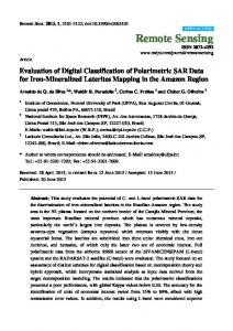
Figure 1. Optical image of Oberpfaffenhofen

The GMM algorithm can be summarized in 4 steps:

1. Initialize K means vectors, K covariance matrix randomly 1 . Then and make the distribution probabilities πk equals to K calculate the initial log likelihood. 2. E step. Evaluate the posterior probabilities γ(znk ) shown in (19) using the current parameters µk , Σk and πk . 3. M step. Calculate the new parameters µnew , Σnew and k k new πk with equations (21), (22) and (23). 4. Repeat steps 2 and 3 until complete one of this two conditions: either the difference between the current and previous log likelihoods values is less than a threshold or the maximum number of iterations is reached.

5. EXPRIMENTAL RESULTS The experimental L-band polarimetric image is acquired by ESAR system. Its size is 1548 x 2816. The test site area is close to Oberpfaffenhofen, Munich, Germany. Fig.1 is optical image from Google Earth of the test site, illustrating an airport, an urban area, farmlands, and forested areas. The standard GMM consists in the use the scattering matrix components Shh , Shv and Svv as feature vector, the image is vectorized into D x N matrix where N is the number of pixels. The mean vectors and covariance matrices are initialized randomly, the number of class K and tolerance are equal to 5 and 0.01 respectively. Fig.2 shows standard GMM classification result. A combination between a decomposition and classification is proposed in this paper. It consists in the use of powers values resulting from improved Freeman decomposition as feature vector in GMM classification with the same number of classes and tolerance. A comparison between these two GMM methods will be performed. Fig.3 shows improved Freeman-GMM classification result.

Figure 2. GMM classification

6. COMPARISON OF THE CLASSIFICATIONS RESULTS Two patches (forest and urban) are taken to compare the two classifications, as shown in Fig.4-c-d. In the case of standard GMM classification, some of building areas are classified correctly with red color, the remaining is labeled as dense forest areas. The urban classification error is about 37 %. The contribution of improved Freeman-GMM algorithm is the fact that it classifies urban, dense forest and less dense forest areas with red, green and Black colors respectively. Hence the result is more smooth and the urban area classification error is reduced to


343


Figure 3. Improved Freeman-GMM classification

(a)

(b)

(c)

(d)

(e)

(f)

about 13 %. Confusion matrices in Table.1 and Table.2 shows that the total contribution of the new combination is over 5 %.

Urban Farm Dense forest Road Less dense forest Kappa

Urban

Farm

Dense forest

Road

0.6043 0

0.0053 0.8142

0.3619 0

0 0.1284

Less dense forest 0.0285 0.0574

0.0066

0.0049

0.8262

0

0.1022

0

0.0054

0

0.9946

0

0

0.1946

0.0953

0.0097

0.7004

0.8304

Figure 4. Comparison between GMM and Improved FreemanGMM: Google Earth, (a) Urban area and (b) Forested area. Standard GMM classification, (c) Urban area with and (d) Forested area. Improved Freeman GMM classification, (e) Urban area and (f) Forested area

Table 1. Standard GMM confusion matrix

Urban Farm Dense forest Road Less dense forest Kappa

7. CONCLUSION

Urban

Farm

Dense forest

0.8340 0

0.0325 0.9841

0.1223 0

0 0.0159

Less dense forest 0.0112 0

0

0

1

0

0

0

0.0232

0

0.9768

0

0.0415

0.2878

0.0643

0

0.6064

Road

In this paper, a new combination between improved Freeman decomposition and the unsupervised Gaussian mixture model (GMM) classification is proposed. Standard GMM classification fails to distinguish between forest and urban areas. Experimental results show that the proposed combination works better than standard GMM classification alone. Using the proposed method, different patterns became more homogeneous and clearly delimitated and the confusion encountered with standard GMM classification has been removed. The kappa coefficient value has been improved as well. REFERENCES

0.8888

Table 2. Improved Freeman-GMM confusion matrix

An, W., Cui, Y. and Yang, J., 2010. Three-component modelbased decomposition for polarimetric sar data. IEEE Transac-


344


tions on Geoscience and Remote Sensing 48(6), pp. 2732–2739. Bishop, C., 2006. Pattern Recognition and Machine Learning. Information Science and Statistics, Springer. Freeman, A. and Durden, S. L., 1998. A three-component scattering model for polarimetric sar data. IEEE Transactions on Geoscience and Remote Sensing 36(3), pp. 963–973. Huynen, J., 1970. Phenomenological theory of radar targets. Drukkerij Bronder-Offset N.V. Lee, J. and Pottier, E., 2009. Polarimetric Radar Imaging: From Basics to Applications. Optical Science and Engineering, CRC Press.


345