features of the sequence for space-time invariant classification [1], however they ... neural network techniques can allow non-stationary series to be modelled ...
Pre-processing inputs for optimally-configured timedelay neural networks T.Taskaya-Temizel, M.C.Casey, and K.Ahmad
A procedure for pre-processing non-stationary time series is proposed for modelling with a time-delay neural network (TDNN).
The procedure
stabilises the mean of the series and uses a Fast Fourier Transform (FFT) to determine the TDNN input size. Results of applying this procedure on five well-known data sets are compared with existing hybrid neural network techniques, demonstrating improved prediction performance. Introduction: The learning of a temporal sequence of events is essential for a number of applications in physics, electronics and neurobiology. Time-delay neural networks (TDNN) can learn to detect (a) position independent features within a sequence, and (b) non-linear features of the sequence for space-time invariant classification [1], however they have difficulty in modelling, and hence predicting from, non-stationary data.
Natural temporal
sequences tend to include trend, seasonality and variance change, and it is important to quantify and, if possible, eliminate these before developing a model. Whilst some hybrid neural network techniques can allow non-stationary series to be modelled directly [2,3,4,5], they add a degree of complexity to the modelling process and are difficult to apply.
In
contrast, pre-processing techniques can be used to stabilise the mean and variance of a series [6], but the choice of technique is controversial [2]. We describe a new procedure for stabilising a time series for which the choice of pre-processing technique is optimised for a TDNN. Furthermore, the configuration of the TDNN is determined directly from the time series. A TDNN is a variant of the multi-layer perceptron in which the inputs to any node i can consist of the outputs of the earlier nodes generated between the current step t and step t-d, where
d ∈ Z + ∀d < t . Here, the activation function for node i at time t is:
1
y i (t ) = f
����
��� M
�
T
j =1 n =1
wij (t − n) y j (t − n)
�
(1)
where yi(t) is the output of node i at time t, wij(t) is the connection weight between node i and j at time t, T is the number of tap delays, M is the number of nodes connected to node i from preceding layer, and f is the activation function, typically the logistic sigmoid. In order to train the TDNN, it is necessary to filter any change in the variance or mean from the sequence. Indeed, the elimination of variance and mean change, if at all possible, is the premise for modelling the behaviour of a temporal sequence. This is particularly important as some time series exhibit long-term cyclical behaviour, which is often ignored. Furthermore, as for other types of neural network, a TDNN cannot predict trend because the output of the network is typically computed using a threshold function, with the output of the function bounded to values, say, between 0 and 1 [7]. Autoregressive models, such as the seasonal autoregressive integrated moving average model (SARIMA), have been used to generate deseasonalised and de-trended time series, with the residuals used to train a TDNN, obtaining good results [2,3,4]. In this letter we present a pre-processing method that can be used to stabilise a time series appropriately for the application of a TDNN. The prediction capability of a TDNN trained with this stabilised data compares well to that of SARIMA and other neural network hybrids. Method: The procedure for stabilising a time series follows: VL Step 1: Given a time series {xi }iK=1 , create training {xi }TR i =1 , validation {xi }i =TR and test data sets
{xi }iK=VL , where i is the time index.
Step 2: Stabilise the variance of {xi }VL i =1 using the Box-Cox power transformation:
�� ( x
x ' = � i
p i
− 1) / p , p ≠ 0
log( x i ), p = 0
(2)
where the parameter p is computed to maximise log-likelihood. Note, if p is in the 95% confidence interval, there is strong evidence that the data should be analysed after first performing a power transformation [8]. Step 3: Adjust the mean of the series by computing first-order difference:
xi''+1 = xi'+1 − xi'
(3)
2
Step 4: Normalise the series by computing z-scores:
xi'' − x ''
zi = where
(4)
σ x"
x '' is the mean, and σ x '' the variance, of {xi''}VL i =1 .
Step 5: Estimate the number of delays (IL) in the input layer by computing the Fast Fourier Transform (FFT) of
{xi }VL i =1 : VL
Xi = where
wVL = e ( −2π
response of
i ) / VL
j =1
th
is a VL
( j −1)(i −1) x j wVL
root of unity. Let
(5)
Ri = X i be the amplitude
X i . Then set IL to be the period of the maximum power of Ri . In order
to ensure that there are sufficient elements to the input, the number IL is limited to be less than VL/4. This restriction is based upon empirical evidence from a variety of seasonal time series and appears not to restrict training. Step 6: Restrict the number of output nodes to unity and set the hidden layer size (HL):
HL ≤
(IL + 1) 2
(6)
Once the time series has been stabilised, then a TDNN with IL input nodes, HL hidden nodes, and 1 output node (IL:HL:1) can be built. Here, the prediction window is ‘one-step’ ahead only, where the last IL values of the time series are used to predict just the next value. Experiments and results: In order to evaluate the pre-processing and TDNN configuration selection method proposed, we performed a number of experiments with TDNN i
j
configurations of 2 : 2 :1, where i and j were varied between 1 and 5, and hence with 256 networks ranging from 2:2:1 to 32:32:1 in configuration. Each configuration was tested with 30 different random initial conditions to provide an average root mean square error (RMSE). A hyperbolic tangent activation function was used for the hidden layers and linear function for the output layer, with the network trained using the gradient descent algorithm for a maximum of 20,000 epochs. The initial learning rate parameter λ= 0.1 was increased by 1.05% if the training error decreased, otherwise was decreased by 0.7%, if the training error increased by over 4%. Training was stopped if the validation error increased 600 consecutive times.
3
We compared our results with that of results obtained from the hybrid ARIMA-NN model of Zhang and Qi [2]. Here, they use a first order polynomial fit to de-trend, and an ARIMA variant to de-seasonalise the data. They evaluated their method on five data sets, each of which are known to have well-behaved trend and seasonality: US Bureau of Census (USBC) retail, hardware, clothing, furniture, and the well-known sunspot data. Following our method, the FFT analysis of these data sets was used to determine the dominant cycles, which for the four USBC data sets were between 11 and 12, matching the intuitive monthly period of the data. For each data set, Table 1 shows the mean RMSE for the TDNN trained on data preprocessed using our technique, compared with the results for the ARIMA-NN technique. For each data set, the TDNN configuration that produced the best mean performance (lowest RMSE) out of the 256 is shown and compared with the corresponding ARIMA-NN model. The TDNN with 14:2:1 and 16:2:1 architectures, trained on the first-order differenced data sets, produce lower RMSE than the hybrid system on the USBC retail (36%) and hardware (27%) data sets. In contrast, the TDNN has higher RMSE for the USBC clothing (-18%) and furniture (-74%) data sets, and for the sunspot data (-8%). Using a first-order polynomial fit to de-trend the data, instead of the first order differencing, produces worse results: retail (-28%), hardware (-5%), furniture (-11%) and sunspot (-3%). For the clothing data set the results were 3% better than with differencing. However, contrary to the hybrid ARIMA-NN technique, the TDNN performs better with first-order differencing, rather than with the polynomial fit. On average, the best-performing configuration for all of the data sets consisted of a 14:2:1 configuration, which is close to the FFT prediction of between 11 and 12, generated using the FFT. Our results show that, on the best-fit results, we obtain a 22% lower RMSE error than the hybrid ARIMA-NN technique, with retail, hardware, clothing, and sunspot giving 47%, 64%, 19.7%, 12% better performance, whilst the furniture results were 28% worse. Our method for the selection of the TDNN configuration also appears to provide near-optimum parameters, as can be seen in Fig. 1, which shows a contour plot of the furniture RMSE for the variation in the input and hidden layer configuration, where darker regions indicate lower final RMSE. Here, the white circle marks the position of the 14:2:1 architecture, as selected by our method, which lies within the optimum region of configuration that gives the lowest RMSE.
4
Conclusion: We have described a procedure for stabilising a time series and designing a corresponding TDNN that can be used to effectively model the series. Our approach is based on a classical first order time-differencing of a time series coupled with a FFT to compute the longest cycle in the series. This approach compares well with reported results that rely more on ad-hoc procedures for pre-processing and configuration, as well as more complex modelling techniques. An extension to this work would be to model local variance changes using other well-established neural architectures, such as the modular mixture-of-experts network.
5
References 1 WAIBEL A., HANAZAWA T., HINTON G., SHIKANO K., LANG K.J.: ‘Phoneme Recognition Using Time-Delay Neural Networks’, IEEE Transactions on Acoustics, Speech and Signal Processing, 1989, 37, 3, pp.328-339. 2 ZHANG G.P., QI M.: ‘Neural network forecasting for seasonal and trend time series’, European Journal of Operational Research, 2005, 160, 2, pp. 501-514. 3 TSENG F-M., YU H-C., TZENG G-H.: ‘Combining neural network model with seasonal time series ARIMA model’, Technological Forecasting and Social Change, 2002, 69, pp.71-87. 4 VIRILI F., FREISLEBEN B.: ‘Nonstationarity and Data Preprocessing for Neural Network Predictions of an Economic Time Series’, Proc. IEEE Conf. On Neural Networks, July 2000, Como, Italy, 5, pp.5129-5136. 5 ZHANG G.P.: ‘Time Series Forecasting using a hybrid ARIMA and neural network model’, Neurocomputing, 2003, 50, pp.159-175. 6 BOX, G. E. P., COX, D. R.: ‘An analysis of transformations’, JRSS B, 1996, 26 pp.211–246. 7 COTTRELL M., GIRARD B., GIRARD Y., MANGEAS M., MULLER C.: ‘Neural Modeling for Time Series: A Statistical Stepwise Method for Weight Elimination’, IEEE Transactions on Neural Networks, 1995, 6, 6, pp. 1355-1364. 8 ATKINSON, A. C.: ‘Plots, Transformations, and Regression’, 1985, Oxford, pp.85-89. Authors’ Affiliations T.Taskaya-Temizel, M.C.Casey and K. Ahmad (Department of Computing, School of Electronics and Physical Sciences, University of Surrey, GU2 7XH, Guildford, United Kingdom) Figure Captions: Fig.1: Contour plot of USBC Furniture testing data performance. Table Captions: Table 1: Comparison of RMSE results for TDNN and hybrid ARIMA-NN architectures.
6
Figure 1:
7
Table 1: Data Set USBC Retail USBC Hardware USBC Clothing USBC Furniture Sunspot
TDNN Configuration 16:2:1 14:4:1 14:2:1 16:2:1 8:2:1
TDNN 628.70 35.70 372.50 173.10 18.09
± ± ± ± ±
28.27 6.90 50.66 31.10 1.86
ARIMANN 975.55 49.17 315.43 99.45 16.73
8