PHYSICS OF FLUIDS
VOLUME 13, NUMBER 3
MARCH 2001
Boundary-layer thickness and instabilities in Be´nard convection of a liquid with a temperature-dependent viscosity Michael Mangaa) and Dayanthie Weeraratne Department of Geological Sciences, University of Oregon, Eugene, Oregon 97403
S. J. S. Morris Department of Mechanical Engineering, University of California, Berkeley, California 94720
共Received 8 February 2000; accepted 4 December 2000兲 New and published experimental measurements of spatial and temporal aspects of variable-viscosity convection are compared with boundary layer models. Viscosity is assumed to decrease with increasing temperature T so that convection occurs beneath a relatively stagnant layer. Of particular interest to applications involving asymptotically large viscosity variations, is the result that both the temperature difference across the hot thermal boundary layer and the frequency of thermal formation scale with the rheological temperature scale ⫺(d log /dT)⫺1. Measurements indicate that for large Rayleigh numbers, viscosity varies by less than a factor of ⬇37 across the actively convecting region. © 2001 American Institute of Physics. 关DOI: 10.1063/1.1345719兴
that inertial effects can be neglected, i.e., Pr is sufficiently large that the Reynolds number Re is less than 1. Morris and Canright4 present a boundary layer analysis of variable viscosity convection for the case in which viscosity depends exponentially on temperature T,
When natural thermal convection occurs in a highly viscous liquid, or in a solid deforming by diffusion creep, the viscosity can increase by many orders of magnitude from the hottest to the coldest parts of the flow. In applications to the interiors of planets such as Venus,1 the geometry can be modeled to a first approximation as Be´nard convection, i.e., a plane layer of thickness D with two horizontal isothermal boundaries at temperatures T H and T C 共see Fig. 1兲. For large Rayleigh numbers, Ra, the convecting fluid can be divided into three regions: a well-mixed interior in which the horizontally averaged temperature T i is approximately constant, and two thermal boundary layers, with thicknesses ␦ C and ␦ H , across which most of the temperature change occurs. In a uniform-viscosity Boussinesq fluid with no-slip upper and lower boundaries, the symmetry of the problem requires that T i ⫽(T C ⫹T H )/2 and ␦ C ⫽ ␦ H . In a fluid with a temperature-dependent viscosity, however, T i is no longer the mean of the T C and T H 共Ref. 2兲. Instead, marginal stability analysis,3 boundary-layer analysis,4 laboratory experiments,5 and numerical simulations6,7 indicate that convection occurs beneath a stagnant lid that forms below the cold upper boundary. In the upper thermal boundary layer, only a fraction of the temperature difference T i ⫺T C is thus able to drive convection, whereas in the bottom thermal boundary layer the entire temperature difference T H ⫺T i is involved. Richter et al. 共Ref. 8, p. 191兲 note that ‘‘the usefulness of representing a variable-viscosity system in terms of a convective layer below a stagnant lid depends on understanding or being able to predict the relative thickness of the layers.’’ Accordingly, in this brief communication, we compare laboratory experiments and theoretical models of temperature-dependent viscosity convection. We focus on the limit of effectively infinite Prandtl number Pr⫽ / so
⫽ C e ⫺ ␥ (T⫺T C ) ,
which is a reasonable approximation for many liquids. It will be convenient for our discussion to define ⫽ C / H to be the ratio of viscosities at the temperatures T C and T H . Applying free-slip boundary conditions along with the assumption that flow is two dimensional and steady, Morris and Canright4 made the generalizable prediction that convection is confined to region across which temperature varies by O( ␥ ⫺1 ). A corollary is then
␥ 共 T H ⫺T i 兲 →constant as →⬁.
共2兲
Part of the upper boundary layer 共region ␦ C⬘ in Fig. 1兲 is thus effectively rigid below a critical temperature that is a property of both the material and the boundary temperature. Figure 2共a兲 shows a compilation of experimentally determined values of ␥ (T H ⫺T i ) as a function of ; only experiments with Nusselt numbers Nu⬎4.5 are shown. Because Eq. 共1兲 only approximates the temperature-dependent viscosity of the fluids used in the laboratory experiments,2,8–12 we evaluate ␥ ⫽⫺d log /dT at T⫽T H 共Ref. 13兲. Figure 2共a兲 provides the first direct experimental confirmation that the asymptotic limit given by Eq. 共2兲 is reached for ⬎O(103 ), and thus complements the results of numerical studies.7,14 For smaller viscosity variations (→1), it is possible to estimate the relative thickness of thermal boundary layers. In
a兲
Author to whom correspondence should be addressed; electronic mail:
[email protected]
1070-6631/2001/13(3)/802/4/$18.00
共1兲
802
© 2001 American Institute of Physics
Downloaded 25 Nov 2001 to 128.32.149.194. Redistribution subject to AIP license or copyright, see http://ojps.aip.org/phf/phfcr.jsp
Phys. Fluids, Vol. 13, No. 3, March 2001
FIG. 1. Vertical temperature distribution; ␦ denotes boundary layer thicknesses, z is the vertical position, T is temperature, and is the dimensionless temperature.
flows with no-slip boundaries, the thermal boundary layer thickness ␦ scales with Pe1/3 共e.g., Ref. 15兲, where Pe is the Peclet number. The scaling derived by Solomatov16 for freeslip surfaces becomes
FIG. 2. 共a兲 ␥ (T H ⫺T i ) 关see Eq. 共2兲兴 as a function of the viscosity ratio ⫽ C / H for published experimental data 共Refs. 9–12兲. 共b兲 Dimensionless interior temperature 共see Fig. 1兲 as a function of for published experimental data 共Refs. 8–12兲. The solid curve is given by Eq. 共3兲. For Ref. 8, data with Ra⬎4⫻104 is shown. Re⬍1 for all experiments except those of Zhang et al. 共Ref. 12兲. (T) for the glycerol used by Zhang et al. 共Ref. 12兲 is from Ref. 19.
Thermal boundary layers in variable-viscosity convection
803
FIG. 3. Period of thermal formation (t * ) from the hot boundary layer as a function of the Rayleigh number based on properties of the lower thermal boundary layer 关see Eq. 共5兲兴. Numbers next to the data points are the viscosity ratios . The solid line is t * ⫽D 2 (Ra␦ /Racr) ⫺2/3/2.77 共from Ref. 22兲, with Racr⫽1700. Inset: t * as a function of Ra␥ .
i⬇
1 1⫹ ⫺1/6
共3兲
for no-slip surfaces.11 Equation 共3兲 is identical to the relationship of Wu and Libchaber,17 which is based on the assumption of equivalent temperature scales and viscous stresses18 in both thermal boundary layers. Figure 2共b兲 shows that Eq. 共3兲 agrees with published experimental data for ⬍O(102 ). Overall, Fig. 2 suggests that straightforward boundary layer arguments, used to derive Eqs. 共2兲 and 共3兲, describe some features of thermal boundary layers in variable-viscosity convection. Two additional features of the results in Fig. 2 are of interest. First, the data in Fig. 2 have no dependence on the Rayleigh number 共Ra varies by about 5 orders of magnitude兲; see also Ref. 14. Second, Re⬍1 for all the data in Fig. 2 except that of Zhang et al.,12 for which Re is between about 1 and 100. Thus fluid inertia does not seem to affect the relationship between i and . At sufficiently high Ra, ⬎O(105 ), Be´nard convection typically becomes unsteady, and the unsteadiness is often accompanied by rising and sinking thermals of relatively hot and cold fluid, respectively. We performed a set of experiments to measure the frequency of thermal formation in fully developed Be´nard convection. Experiments are performed in a tank with D⫽17 cm and a square base 34 ⫻ 34 cm. Sidewalls are insulated. The working fluid is corn syrup with 3% added water. Details of the experimental setup, procedure, and data are published in a thesis.20 The period of hot thermal formation, t * , is determined from spectral analysis of temperature measurements recorded by two thermocouples located 1 cm above the base of the tank that recorded the passage of hot thermals. Measurements are made once ‘‘equilibrium’’ is reached; this is identified by requiring that the time-averaged T i is constant. Thermocouples record temperatures at 1–3 s intervals over at least 10 periods 共4–12 h兲. We confirm visually that thermals did indeed form in all experiments. Figure 3 shows t * as a function of a suitably defined Ra. For the case of variable-viscosity convection, Ra should be
Downloaded 25 Nov 2001 to 128.32.149.194. Redistribution subject to AIP license or copyright, see http://ojps.aip.org/phf/phfcr.jsp
804
Phys. Fluids, Vol. 13, No. 3, March 2001
Manga, Weeraratne, and Morris
based on an appropriate choice of and temperature difference ⌬T driving motion. Here we consider two definitions of Ra. First, in the limit →⬁, ⌬T scales with ␥ ⫺1 , and we can define Ra based on properties of the hot boundary layer as
g ␣␥ ⫺1 D 3 Ra␥ ⫽ , H
共4兲
where , g, , and ␣ are density, gravitational acceleration, thermal diffusivity, and thermal expansivity, respectively, and H ⫽ (T H ). Previous studies2,3,8,9 have suggested that a suitable choice of viscosity is the value based on the mean of the boundary temperatures 共the so-called film temperature兲. With this choice of viscosity,3 the critical Ra for the onset of convection, Racr , varies by less than about 50% for 1⬍ ⬍106 . A second suitable definition of Ra is thus
g ␣ 共 T H ⫺T i 兲 D 3 Ra␦ ⫽ , ␦ H
共5兲
where ␦ H ⫽ (0.5关 T i ⫹T H 兴 ). A best fit to the six measurements in Fig. 3 gives t * ⬀Ra␦⫺0.58 and t * ⬀Ra␥⫺0.61 . Despite the wide range of , t * scales with Ra␦ and Ra␥ indicating that the processes responsible for the formation of thermals are local to the hot boundary layer. Howard21 described a mechanistic process for the formation of thermals in high Pr flows that involves the conductive growth of a thermal boundary layer, followed by the relatively rapid release of fluid from the layer once the local Rayleigh number 共based on the boundary layer thickness兲 exceeds Racr . Thermals formed through this mechanism will have t *⬀
D2 共 Ra/Racr兲 ⫺2/3,
共6兲
where Ra is given by Eq. 共4兲 or 共5兲. Sparrow et al.22 measured the frequency of thermal formation above a heated surface; their best-fit relationship, shown in Fig. 3 for comparison, is compatible with our measurements. Figure 3 thus suggests that thermals in fully developed variable-viscosity convection may form by the processes described by Howard,21 at least in low Re flows. We therefore have a basis for using Eqs. 共4兲–共6兲 for extrapolating to the interior of planets. We can also use the temporal variations of temperature to obtain additional information about the time-averaged thickness of thermal boundary layers. At sufficiently high Rayleigh numbers 关 Ra⬎O(106 ), where Ra is based on the viscosity at the mean of T C and T H ] flow is dominated by rising and falling thermals. In this limit, the mean temperature at a depth D/2 is the same at all horizontal positions,10 and the large-scale flow observed at higher Re 共Ref. 12兲 is not apparent if Re⬍1. The inset of Fig. 4 shows histograms 共analogous to probability distributions functions兲 of temperatures recorded from an array of six thermocouples located at z⫽D/2 共see Fig. 1兲. Here, histograms are normalized to have a maximum value of 1. We choose three experiments for which Ra and Nu are similar but , and thus T i , are different 共experiments 25–27
FIG. 4. Histograms of temperature in the middle of the convecting fluid for temperature normalized as (T⫺T i )/(T H ⫺T i ). Ra is based on the viscosity at the mean of T C and T H 共see Refs. 2 and 3, and 8 and 9兲. Inset: Histograms of temperature in the middle of the convecting fluid with temperature normalized as ⫽(T⫺T C )/(T H ⫺T C ).
of Ref. 11兲. In Fig. 4, T is normalized by the temperature difference across the hot thermal boundary layer and the histograms collapse to a single curve. Figure 4 thus shows that the temperature difference across the active part of the cold boundary layer 共region ␦ C⬙ ) scales with that across the hot boundary layer 共region ␦ H ). In detail, for the three experiments shown in Fig. 4, the mean temperature anomaly of the cold thermals is ⫺1.5 times the temperature anomaly of the hot thermals. Experimental5 and numerical23 studies of transient convection beneath a cooled surface indicate that a stagnant layer develops once the viscosity ratio across the cold thermal boundary layer exceeds about 10 ( ␥ ⌬T⬇2.2). This result, combined with Fig. 2共a兲 ( ␥ 关 T H ⫺T i 兴 ⬇1.4 for large ), implies that the viscosity ratio across the actively convecting fluid is ⬇37 for Ⰷ1. The uppermost part of the fluid 共region ␦ C⬘ in Fig. 1兲 must therefore be stagnant1–9 and flow beneath the stagnant layer more closely resembles isoviscous convection driven by a temperature difference O( ␥ ⫺1 ). 4,7 Although we have only presented results for fully developed Be´nard convection, the scaling relationships illustrated in Figs. 2 and 3 apply to internally heated flows,23 transient convection,24 and other convective phenomena.25 ACKNOWLEDGMENTS
This work was supported by NSF through Grant No. EAR9701768 and REU supplements. The authors thank M. Jellinek for comments. 1
V. S. Solomatov and L. N. Moresi, ‘‘Stagnant lid convection on Venus,’’ J. Geophys. Res. 101, 4737 共1996兲. 2 J. R. Booker, ‘‘Thermal convection with strongly temperature-dependent viscosity,’’ J. Fluid Mech. 76, 741 共1976兲. 3 K. C. Stengel, D. S. Oliver, and J. R. Booker, ‘‘Onset of convection in a variable-viscosity fluid,’’ J. Fluid Mech. 120, 411 共1982兲. 4 S. Morris and D. Canright, ‘‘A boundary layer analysis of Be´nard convection in a fluid of strongly temperature-dependent viscosity,’’ Phys. Earth Planet. Inter. 36, 355 共1984兲.
Downloaded 25 Nov 2001 to 128.32.149.194. Redistribution subject to AIP license or copyright, see http://ojps.aip.org/phf/phfcr.jsp
Phys. Fluids, Vol. 13, No. 3, March 2001 5
A. Davaille and C. Jaupart, ‘‘Transient high-Rayleigh-number thermal convection with large viscosity variations,’’ J. Fluid Mech. 253, 141 共1993兲. 6 M. Ogawa, G. Schubert, and A. Zebib, ‘‘Numerical simulations of threedimensional thermal convection in a fluid with strongly temperaturedependent viscosity,’’ J. Fluid Mech. 233, 299 共1991兲. 7 L.-N. Moresi and V. S. Solomatov, ‘‘Numerical investigation of 2D convection with extremely large viscosity variations,’’ Phys. Fluids 7, 2154 共1995兲. 8 F. M. Richter, H. Nataf, and S. F. Daly, ‘‘Heat transfer and horizontally averaged temperature of convection with large viscosity variations,’’ J. Fluid Mech. 129, 173 共1983兲. 9 E. Giannandrea and U. Christensen, ‘‘Variable viscosity convection experiments with a stress-free upper boundary and implications for the heat transport in the Earth’s mantle,’’ Phys. Earth Planet. Inter. 78, 139 共1993兲. 10 D. Weeraratne and M. Manga, ‘‘Transitions in the style of mantle convection at high Rayleigh numbers,’’ Earth Planet. Sci. Lett. 160, 563 共1998兲. 11 M. Manga and D. Weeraratne, ‘‘Experimental study of non-Boussinesq Rayleigh–Be´nard convection at high Rayleigh and Prandtl numbers,’’ Phys. Fluids 11, 2969 共1999兲. 12 J. Zhang, S. Childress, and A. Libchaber, ‘‘Non-Boussinesq effect: Thermal convection with broken symmetry,’’ Phys. Fluids 9, 1034 共1997兲. 13 A. Ansari and S. Morris, ‘‘The effects of a strongly temperaturedependent viscosity of Stokes drag law: Experiments and theory,’’ J. Fluid Mech. 159, 459 共1985兲. 14 R. A. Trompert and U. Hansen, ‘‘On the Rayleigh number dependence of convection with a strongly temperature-dependent viscosity,’’ Phys. Fluids 10, 351 共1998兲. 15 A. Acrivos and J. D. Goddard, ‘‘Asymptotic expansions for laminar con-
Thermal boundary layers in variable-viscosity convection
805
vection heat and mass transfer,’’ J. Fluid Mech. 23, 273 共1965兲. V. S. Solomatov, ‘‘Scaling of temperature- and stress-dependent viscosity convection,’’ Phys. Fluids 7, 266 共1995兲. 17 X.-Z. Wu and A. Libchaber, ‘‘Non-Boussinesq effects in free thermal convection,’’ Phys. Rev. A 45, 1283 共1991兲. 18 J. Zhang, S. Childress, and A. Libchaber, ‘‘Non-Boussinesq effect: Asymmetric velocity profiles in thermal convection,’’ Phys. Fluids 10, 1534 共1998兲. 19 T. E. Daubert and R. P. Danner, Physical and Thermodynamic Properties of Pure Chemicals. Data Compilation 共Taylor and Francis, Washington, DC, 1996兲. 20 D. Weeraratne, ‘‘Convective heat transport in high Prandtl number fluids and planetary mantles,’’ M.Sc. thesis, University of Oregon, 1999, 179 pp. 21 L. N. Howard, ‘‘Convection at high Rayleigh number,’’ in Proceedings of the 11th International Congress Applied Mechanics, edited by H. Go¨rtler 共Springer, Berlin, 1964兲. 22 E. M. Sparrow, R. B. Husar, and R. J. Goldstein, ‘‘Observations and other characteristics of thermals,’’ J. Fluid Mech. 41, 793 共1970兲. 23 O. Grasset and E. M. Parmentier, ‘‘Thermal convection in a volumetrically heated, infinite Prandtl number fluid with strongly temperaturedependent viscosity: Implications for planetary thermal evolution,’’ J. Geophys. Res. 103, 18171 共1998兲. 24 A. Davaille and C. Jaupart, ‘‘Onset of thermal convection in fluids with a temperature dependent viscosity: Application to the oceanic mantle,’’ J. Geophys. Res. 99, 19853 共1994兲. 25 W. B. Moore, G. Schubert, and P. Tackley, ‘‘Three-dimensional simulations of plume-lithosphere interaction at the Hawaiian swell,’’ Science 279, 1008 共1998兲. 16
Downloaded 25 Nov 2001 to 128.32.149.194. Redistribution subject to AIP license or copyright, see http://ojps.aip.org/phf/phfcr.jsp