PHYSICS OF FLUIDS
VOLUME 13, NUMBER 5
MAY 2001
Application of reduced-order controller to turbulent flows for drag reduction Keun H. Lee, Luca Cortelezzi,a) John Kim,b) and Jason Speyer Department of Mechanical & Aerospace Engineering, University of California, Los Angeles, California 90095
共Received 18 April 2000; accepted 29 January 2001兲 A reduced-order linear feedback controller is designed and applied to turbulent channel flow for drag reduction. From the linearized two-dimensional Navier–Stokes equations a distributed feedback controller, which produces blowing/suction at the wall based on the measured turbulent streamwise wall-shear stress, is derived using model reduction techniques and linearquadratic-Gaussian/loop-transfer-recovery control synthesis. The quadratic cost criterion used for synthesis is composed of the streamwise wall-shear stress, which includes the control effort of blowing/suction. This distributed two-dimensional controller developed from a linear system theory is shown to reduce the skin friction by 10% in direct numerical simulations of a low-Reynolds number turbulent nonlinear channel flow. Spanwise shear-stress variation, not captured by the distributed two-dimensional controller, is suppressed by augmentation of a simple spanwise ad hoc control scheme. This augmented three-dimensional controller, which requires only the turbulent streamwise velocity gradient, results in a further reduction in the skin-friction drag. It is shown that the input power requirement is significantly less than the power saved by reduced drag. Other turbulence characteristics affected by these controllers are also discussed. © 2001 American Institute of Physics. 关DOI: 10.1063/1.1359420兴 I. INTRODUCTION
termines the optimal control input by minimizing the cost functional for a short time interval, was successfully applied to the stochastic Burger’s equation.7 Bewley and Moin8 extended the suboptimal control to a turbulent channel flow. This method, however, requires information about the whole flow field and excessive computation, so that it is impossible or at best extremely difficult to implement. It is necessary to develop a control scheme that utilizes easily measurable quantities. Lee et al.9 developed a neural network control algorithm that approximates the correlation between the wall-shear stresses and the wall actuation and then predicts the optimal wall actuation to produce the minimum value of skin friction. They also produced a simple control scheme from this neural network control, which determines the actuation as the sum of the weighted spanwise wall-shear stress, w/ y 兩 w . Recently, Koumoutsakos10 reported a substantial drag reduction obtained by applying a feedback control scheme based on the measurement and manipulation of the wall vorticity flux. Furthermore, he showed that the strength of unsteady mass transpiration actuators can be derived explicitly by inverting a system of equations. Other systematic controls11–17 have been developed by exploiting the tools recently developed in the control community.18–21 Joshi et al.11–13 and Bewley and Liu14 developed an integral feedback controller, a linear quadratic 共LQ兲 controller, and an H⬁ controller 共worst-case controller兲 to successfully stabilize unstable disturbances in transitional flow. In particular, Cortelezzi and Speyer15 introduced the multi-input–multi-output 共MIMO兲 linear-quadratic-Gaussian 共LQG兲/loop-transfer-recovery 共LTR兲 synthesis,22 combined with model reduction techniques, for designing an optimal linear feedback controller. This controller successfully sup-
Much attention has been paid to the drag reduction in turbulent boundary layers. Skin friction drag constitutes approximately 50%, 90%, and 100% of the total drag on commercial aircraft, underwater vehicles, and pipelines, respectively.1 The decrease of skin friction, therefore, entails a substantial saving of operational cost for commercial aircraft and submarines. Recent reviews1–3 summarize achievements and open questions in boundary layer control. With the notion that near-wall streamwise vortices are responsible for high skin friction in turbulent boundary layers, Choi et al.4 manipulated the near-wall turbulence by applying various wall actuations. They achieved a 20% skinfriction reduction in a turbulent channel flow by applying a wall transpiration equal and opposite to the wall–normal velocity component measured at y ⫹ ⫽10. This control is shown to effectively make the streamwise vortices weaker. However, it is not easily implementable since it is difficult to place sensors inside the flow field. Other attempts at weakening the near-wall streamwise vortices have been made by imposing spanwise oscillation of the wall5 and using external body force.6 These methods, however, require a large amount of input energy. A reduction in skin friction must be accompanied with the required input energy much less than the energy saved by the reduction. A systematic approach, not relying on physical intuition, has been tried in the past. A suboptimal control, which dea兲
Present address: Department of Mechanical Engineering, McGill University, Montreal, Quebec, Canada; electronic mail:
[email protected] b兲 Author to whom correspondence should be addressed. Telephone: 共310兲 825-4393; fax: 共310兲 206-4830; electronic mail:
[email protected]
1070-6631/2001/13(5)/1321/10/$18.00
1321
© 2001 American Institute of Physics
Downloaded 05 Jul 2001 to 128.97.2.217. Redistribution subject to AIP license or copyright, see http://ojps.aip.org/phf/phfcr.jsp
1322
Lee et al.
Phys. Fluids, Vol. 13, No. 5, May 2001
pressed near-wall disturbances, thus preventing a transition in two-dimensional laminar channel flows. This reducedorder controller16 was applied to two-dimensional nonlinear transitional flows, illustrating that the controller designed from the linear model works remarkably well in nonlinear flows. Our purpose in the present study is to develop a realistic robust optimal controller that systematically determines the wall actuation, in the form of blowing and suction at the wall, relying only on a measured streamwise velocity gradient to reduce skin friction in a fully developed turbulent channel flow. A dynamic representation of the flow field is required for controller design. Due to the complexity and nonlinearity of the Navier–Stokes equations, it is difficult to derive model-based controllers. Therefore, the linearized Navier–Stokes equations for Poiseuille flow are used as an approximation of the flow field and form the basis of system modeling. Several investigators 共e.g., Farrel and Ioannou,23 Kim and Lim,24 to name a few兲 have shown that linearized models have a direct relevance to turbulent flows. A reducedorder controller has been designed based on this model and applied to linear and nonlinear transitional flows.15–17 Encouraged by these results, in this paper we apply this distributed two-dimensional controller to a direct numerical simulation of turbulent channel flow at a low Reynolds number. We then augment our two-dimensional distributed controller by including an ad hoc control scheme to attenuate the residual disturbances in the spanwise direction. In Sec. II, we derive the state-space equations from the linearized two-dimensional Navier–Stokes equations. In Sec. III, we reduce the order of the state-space equations and derive a reduced-order two-dimensional controller by using LQG/LTR synthesis. In Sec. IV, we construct and apply the distributed two-dimensional controller based on the linearized Navier–Stokes equations to a fully developed turbulent channel flow at Re ⫽100, where Re is the Reynolds number based on the wall-shear velocity, u , and the halfchannel height, h. In Sec. V, this distributed two-dimensional controller augmented with a simple ad hoc control scheme is applied to the same flow. In Sec. VI, we present turbulence statistics associated with the controlled flows followed by conclusions in Sec. VII. In this paper, we use (u, v ,w) to represent the velocity components in the streamwise (x), wall–normal (y), and spanwise (z) directions, respectively. II. THE STATE-SPACE EQUATIONS
One of the goals in the present study is to reduce the size of the controller. A controller with a large number of states is of no practical interest in engineering applications because of the amount of hardware and computer power necessary to compute a real-time control law. Consequently, it is crucial to reduce the order of the controller. Figure 1 shows the configuration of the turbulent channel flow equipped with the controller tested for our study. Low-order controllers are usually preferred to high-order one because of the lower cost of hardware construction as well as the less computation time necessary to provide the control
FIG. 1. Schematic representation of turbulent channel flow equipped with sensors and actuators distributed in the streamwise direction in each z plane.
input. Hence, we slice the channel with xy planes equally spaced in the z direction in order to reduce the order of the controller. We then construct the distributed twodimensional controller by applying the two-dimensional controller developed from the linearized two-dimensional Navier–Stokes equations15 to each plane. It is shown16 that the two-dimensional controller is effectively able to reduce the skin-friction drag of the finite-amplitude disturbances in a two-dimensional channel flow. We follow the same derivation of the state-space equation as given in Cortelezzi et al.16 We give a brief outline here for completeness; the interested reader is referred to Cortelezzi et al.16 for details. The wall transpiration is applied to both top and bottom walls in a fully developed turbulent channel flow. For simplicity, though, we derive the state-space equations assuming that blowing and suction is applied only at the bottom wall. The application of blowing and suction to both walls is a trivial extension. We consider two-dimensional incompressible Poiseuille flow in a periodic channel of streamwise length, L x , and channel height, 2h. The undisturbed velocity field has a parabolic profile with centerline velocity U c . The linearized two-dimensional Navier–Stokes equations can be written in terms of the perturbation streamfunction, , 共 t ⫹U x 兲 ⌬ ⫺U ⬙ x ⫽Re⫺1 ⌬⌬ ,
共1兲
where all variables are normalized with U c and h and Re ⫽U c h/ is the Reynolds number. To suppress perturbations evolving within the bottom boundary layer, we apply blowing and suction at the bottom wall 共see Fig. 1兲. For simplicity, we assume that the actuators are continuously distributed. The corresponding boundary conditions are
Downloaded 05 Jul 2001 to 128.97.2.217. Redistribution subject to AIP license or copyright, see http://ojps.aip.org/phf/phfcr.jsp
Phys. Fluids, Vol. 13, No. 5, May 2001
x 兩 y⫽⫺1 ⫽⫺ v w 共 x,t 兲 ,
y 兩 y⫽⫾1 ⫽ 兩 y⫽1 ⫽0,
Application of reduced-order controller to turbulent flows
共2兲
where the control function v w indicates blowing and suction at the bottom wall. We impose the wall transpiration of zero net mass flux. To detect the near-wall disturbances, we measure the gradient of the streamwise disturbance velocity at given point x⫽x i along the bottom wall 共see Fig. 1兲, z 共 x i ,t 兲 ⫽ y y 兩 y⫽⫺1 .
共3兲
In other words, we measure the first term of the disturbance wall-shear stress, yx ⫽Re⫺1 ( y y ⫺ xx ) 兩 y⫽⫺1 . The second term of the wall-shear stress is zero in the uncontrolled case and is known in the controlled case. ˜ , or cost criterion, to We define a performance index J design a controller for the LQG (H2 ) problem. Since we are interested in suppressing the disturbance wall-shear stress, yx , we define ˜ ⫽ lim J
t f →⬁
冕冕 tf
t
L
0
2 兲 兩 y⫽⫺1 dxdt. 共 2y y ⫹ xx
共4兲
The integrand represents the cost of the disturbance wallshear stress, yx , being different from zero. Moreover, the integrand implicitly accounts for the cost of implementing the control itself. There are two reasons to minimize the cost of the control. In any engineering application the energy available to drive the controller is limited, and a large control action may drive the system away from the region where the linear model is valid. By using the same procedure described in Cortelezzi et al.,16 Eqs. 共1兲–共3兲 are converted into the state-space equations: dx ⫽Ax⫹Bu, dt
z⫽Cx⫹Du,
共5兲
with the initial condition x„0…⫽x0, where x is the internal state vector, u is the control vector, z is the measurement vector. Matrices A,B,C contain the dynamics of the twodimensional plane Poiseuille flow, actuators, and sensors, respectively. Matrix D contains the coupling between sensors and actuators. The cost criterion, Eq. 共4兲, becomes ˜ ⫽ lim J
t f →⬁
冕
t
tf
关 z z⫹u F Fu兴 dt, T
T T
共6兲
where the superscript T denotes a transposed quantity. The matrix F is obtained by spectrally decomposing the last term in the cost criterion, Eq. 共4兲. The advantage of the present formulation is that the whole problem decouples with respect to the wave number when Eqs. 共5兲 and 共6兲 are transformed into Fourier space in the streamwise direction. All matrices in Eqs. 共5兲 and 共6兲 are block diagonal, which allows the above state-space system into equivalent N state-space subsystems.25 For a given wave number, ␣ , the state-space subsystem equations are dx␣ dt
⫽A␣ x␣ ⫹B␣ u␣ ,
z␣ ⫽C␣ x␣ ⫹D␣ u␣ ,
共7兲
1323
with the initial condition x␣ (0)⫽x␣ 0 . It can be shown that the cost criterion, Eq. 共6兲, also decouples with respect to the wave number 共otherwise the wave number decoupling is not possible while the system itself is decoupled兲, and we obtain N performance indexes. For a given wave number, ␣ , the cost criterion is defined as ˜ ␣ ⫽ lim J␣ ⫽ lim J t f →⬁
t f →⬁
冕
t
tf
关 z␣T z␣ ⫹u␣T F␣T F␣ u␣ 兴 dt.
共8兲
Consequently, the design of a two-dimensional controller for the system, Eq. 共5兲, with a specified cost criterion, Eq. 共6兲, has been reduced to the independent design of N single-wave number controllers for the subsystems, Eq. 共7兲, along with Eq. 共8兲.
III. MODEL REDUCTION AND CONTROLLER DESIGN
In this section we derive a lower-order two-dimensional controller in two steps.15 First, we construct a lower-order model of Eq. 共7兲, and subsequently, design a single-wave number controller for the reduced-order model. To obtain a lower-order model, we transform Eq. 共7兲 into a Jordan caˆ ␣ ,D␣ that describe the ˆ ␣ ,Bˆ␣ ,C nonical form. The matrices A dynamics of the reduced-order model are obtained from the matrices, A␣ ,B␣ ,C␣ ,D␣ in the Jordan canonical form by retaining rows and columns corresponding to equally well controllable and observable states. The overcaret denotes the quantities associated with the reduced-order model. Although a rigorous mathematical framework for the design of disturbance attenuation (H⬁ ) linear controllers is provided by the control synthesis theory,18,19 for this study LQG(H2 ) synthesis is preferred. A brief review will be given in a self-contained manner to provide the necessary governing equations for closed-loop stability analysis.20 The LQG problem for each wave number ␣ is formulated as a stochastic optimal control problem described by equations ˆ ␣ xˆ␣ ⫹Bˆ␣ u␣ ⫹⌫␣ w␣ , x˙ˆ ␣ ⫽A ˆ ␣ xˆ␣ ⫹D␣ u␣ ⫹v␣ , zˆ␣ ⫽C
共9兲 共10兲
where ⌫␣ is an input matrix, w␣ and v␣ are both white noise processes with zero means and autocorrelation functions, E 关 w␣ 共 t 兲 w␣T 共 兲兴 ⫽W␣ ␦ 共 t⫺ 兲 , E 关 v␣ 共 t 兲 v␣T 共 兲兴 ⫽V␣ ␦ 共 t⫺ 兲 ,
共11兲
where E 关 • 兴 is the expectation operator averaging over all underlying random variables and ␦ (t⫺ ) is the delta function. Note that W␣ and V␣ , the power spectral densities, will be chosen here as design parameters to enhance system performance. An additional comment on the controller design process will be given at the end of this section. The LQG controller is determined by finding the control action u␣ (Z t ), where Z t ⫽ 兵 z( );0⭐ ⭐t 其 is the measurement history, which minimizes the cost criterion,
Downloaded 05 Jul 2001 to 128.97.2.217. Redistribution subject to AIP license or copyright, see http://ojps.aip.org/phf/phfcr.jsp
1324
Lee et al.
Phys. Fluids, Vol. 13, No. 5, May 2001
t f →⬁
⫻E
The Kalman gain matrix L␣ , constructed to trade the accuracy of the new measurements against the accuracy of the state propagated from the system dynamics, is given by
1
J ␣ ⫽ lim
t f ⫺t
冉冕
tf
t
冊
共 xˆ␣T Q␣ xˆ␣ ⫹2xˆ␣T N␣ u␣ ⫹u␣T R␣ u␣ 兲 d , 共12兲
subject to the stochastic dynamics system model equations ˆ ␣T C ˆ␣, Eqs. 共10兲–共11兲. Note that, from Eqs. 共7兲–共8兲, Q␣ ⫽C T T T ˆ N␣ ⫽C␣ D␣ , and R␣ ⫽D␣ D␣ ⫹F␣ F␣ . The division by (t f ⫺t) ensures that the cost criterion remains finite in the presence of uncertainties in the infinite-time problem (t f →⬁). Note that Eq. 共12兲 can include Eq. 共8兲, where J ␣ ⫽ lim
t f →⬁
1 t f ⫺t
E 关 J␣ 兴 ,
共13兲
and the limit in Eq. 共8兲 is explicitly denoted in Eq. 共13兲. Note that even though the time interval is infinite, the time response is still measured by the eigenvalues of the closedloop system. We consider the infinite-time problem with time-invariant dynamics because the controller gains become constants. By nesting the conditional expectation with respect to Z t within the unconditional expectation of Eq. 共13兲, i.e., E 关 J␣ 兴 ⫽E 关 E 关 J␣ /Z t 兴兴 , where E 关 •/Z t 兴 denotes the expectation (•) conditioned on Z t , the cost criterion can be written as J ␣ ⫽ lim ⫻E
冉冕
t
where P␣ is the error variance in the statistical problem. In the infinite-time stationary formulation, the error P␣ is the solution to the algebraic Riccati equation 共ARE兲, ˆ ␣T V␣⫺1 C ˆ ␣ P␣ ⫽0. ˆ ␣ P␣ ⫹P␣ A ˆ ␣T ⫹⌫␣ W␣ ⌫␣T ⫺P␣ C A
˜ ␣T N␣ u␣ ⫹u␣T R␣ u␣ ⫹tr共 P␣ 兲兴 d 关 ˜x␣T Q␣˜x␣ ⫹2x
ˆ ␣ ,C ˆ ␣ ) observable and (A ˆ ␣ ,Bˆ␣ ) controlIf the system is (A lable, then P␣ is positive definite. Under these assumptions, it can be shown that the difference between the internal state xˆ␣ and the estimate state ˜x␣ , i.e., the error, ˜␣ , e␣ ⫽xˆ␣ ⫺x
共19兲
goes to zero as time goes to infinity. In other words, the evolution equation, e˙␣ ⫽A f e⫹Lˆ␣ ⫹⌫␣ w,
共20兲
is stable, i.e., all the eigenvalues of the matrix, ˆ ␣ ⫺Lˆ␣ C ˆ␣, A f ⫽A
共21兲
have a negative real part. Minimizing the infinite-time cost function J, Eq. 共14兲 subject to Eq. 共15兲 yields the following control law:
冊
,
where ˜x␣ ⫽E 关 xˆ␣ /Z t 兴 is the conditional mean estimate of the state xˆ and P␣ is the conditional error variance. This cost criterion is now minimized subject to the estimation equations discussed below. Note that P␣ does not depend on the control 关see Eq. 共18兲 below兴 and, therefore, does not enter into the optimization process. The solution to the regulator problem20 is a compensator composed of a state reconstruction process, known here as a filter 共in the no-noise case it is known as an observer兲 in cascade with a controller 共see Fig. 1, where E i is the estimator and C i is the controller兲. The state estimate 共conditional mean兲 ˜x␣ is governed by the so-called Kalman filter as
ˆ ␣ 共 xˆ␣ ⫺x ˜␣ ⫽C ˜ ␣ 兲 ⫹v␣ . ␣ ⫽zˆ␣ ⫺z
共15兲
If the reduced-order system were the actual system, then ␣ in Eq. 共15兲 is correct. When the actual system is considered and the filter is implemented based on the reduced-state space, z rather than zˆ is the measurement and the filter residual becomes ˆ ␣˜x␣ ⫺D␣ u␣ . ␣ ⫽z␣ ⫺C
共22兲
ˆ ␣ ⫽R␣⫺1 共 Bˆ␣T S␣ ⫹N␣ 兲 , K
共14兲
ˆ ␣˜x␣ ⫹B ˆ ␣ u␣ ⫹L ˆ ␣ ␣ , ˜x˙ ␣ ⫽A
共18兲
where
t f ⫺t tf
共17兲
ˆ ␣˜x␣ , u␣ ⫽⫺K
1
t f →⬁
ˆ ␣T V␣⫺1 , ˆ ␣ ⫽P␣ C L
共16兲
共23兲
and S␣ is the solution of the algebraic Riccati equation 共ARE兲, ˆ ␣T ⫹Q␣ ⫺ 共 S␣ B␣ ⫹N␣ 兲 R␣⫺1 共 B␣T S␣ ⫹N␣T 兲 ⫽0. 共24兲 ˆ ␣ S␣ ⫹S␣ A A ˆ ␣ is It should be remarked that the control gain matrix K determined from functions only of the known dynamics coˆ ␣ ,Bˆ␣ ) and the weighting in the cost criterion efficients (A (Q␣ ,R␣ ), and not the statistic of the input (V␣ , W␣ 兲. Conˆ ␣ is determined from a performance index as sequently, K ˆ ␣ ,Bˆ␣ ) is Eq. 共12兲, independent of the stochastic inputs. If (A 1/2 ˆ controllable and (A␣ ,Q␣ ) observable, then the loop coefficient matrix, ˆ ␣ ⫺K ˆ ␣ Bˆ␣ , Ac ⫽A
共25兲
is stable and S␣ is positive definite. The controllable and observable conditions can be weakened to stabilizable and detectable.21 When we combine the estimator and the regulator together, the dynamic system composed of the controlled process and filter becomes
冉冊冋 e˙␣
˜x˙ ␣
⫽
Af
0
ˆ ␣C ˆ␣ L
Ac
册冉 冊 冉
冊
e␣ Lˆ␣ v␣ ⫹⌫␣ w␣ ⫹ . ˜x␣ Lˆ␣ v␣
共26兲
Note that any choice of two between e, xˆ␣ , and ˜x␣ produce the same dynamics because they are algebraically related by
Downloaded 05 Jul 2001 to 128.97.2.217. Redistribution subject to AIP license or copyright, see http://ojps.aip.org/phf/phfcr.jsp
Phys. Fluids, Vol. 13, No. 5, May 2001
Eq. 共19兲. Under the above controllability and observability assumptions, A f and Ac have only stable eigenvalues if opˆ ␣ and K ˆ ␣ of Eqs. 共17兲 and 共23兲 are used. If the timal gains L actual linear system is used, then x␣ and the reduced-order state estimate ˜x␣ are used to form the closed-loop dynamic system rather than that given in Eq. 共26兲. The eigenvalues of the dynamical matrix now dictate the system stability and will differ from the ideal case of Eq. 共26兲. The parameters used in our LQG design are now addressed. Since the power spectral density is not known, for simplicity of the design we consider V␣ and W␣ to be of the form V␣ ⫽  I and W␣ ⫽ I, where  and are scalar and I is an identity matrix. Only the ratio of  and is important. ˆ ␣ , loop-transfer recovery Furthermore, by choosing ⌫␣ ⫽B 共LTR兲 of the LQG controller to full-state feedback18 guarantees that robust performance occurs when the process noise power spectral density goes to infinity, i.e., →⬁, provided there exists no nonminimal-phase zero in the plant. In our case, there are no nonminimal-phase zeros and robust performance means approximately obtaining 60° of phase margin and 6 db of the gain margin. Note that the choice of ⌫␣ ˆ ␣ implies that the noise is generated along the wall as is ⫽B the control and could be interpreted as due to wall roughness. Furthermore, the values of and  were determined by tuning the controller in the presence of turbulent flow. The degree of loop transfer recovery varied from controller to controller. As described above using LQG/LTR assumes that the uncertainty is at the wall and effects the dynamics in the same way as the control. Since the system has the same controllability with respect to both the control and disturbances, state-space reduction for controller design was straightforward. This is in contrast to H⬁ control used by Bewley and Liu,14 where uncertainty is assumed uniformly throughout the channel. Since controllability of the disturbances is different from that of the control, model reduction may not be straightforward. Furthermore, robustness in terms of traditional measures of the gain and phase margin in control engineering are also obtained by using LQG/LTR. For these reasons LQG/LTR is used for the present study instead of the unstructured uncertainty H⬁ controllers. Figure 1 links the mathematical formulation to its computational implementation by summarizing in a block diagram the control strategy described above. The twodimensional distributed controller can be programmed in a computer routine whose input is a matrix containing the gradients of the streamwise velocity component and whose output is a matrix containing the blowing and suction at the wall. Each column of the measurement matrices contains the gradients of the streamwise velocity component along the wall at a given spanwise location. Each column is processed in parallel by a fast Fourier transform 共FFT兲 and converted into z␣ ’s. Each single-wave number controller, Eqs. 共9兲– 共10兲, is integrated in time by, for example, a third-order lowstorage Runge–Kutta scheme. The u␣ ’s are computed in parallel. An inverse FFT converts u␣ ’s into the columns of the matrix containing the blowing and suction at the wall along the streamwise direction. This routine can be embedded in
Application of reduced-order controller to turbulent flows
1325
any Navier–Stokes solver able to handle time-dependent boundary conditions for the control of three-dimensional channel flows. Figure 1 also provides the basic architecture for the potential implementation of the present distributed twodimensional controller in practical engineering applications. For instance, the gradients of the streamwise velocity component can be measured by microelectromechanical-systems 共MEMS兲 hot-film sensors.26 For each xy plane, analog-todigital converters 共A/D兲 and digital signal processors 共DSP兲 convert the measured gradients into z␣ ’s. Each single-wave number controller, Eqs. 共9兲–共10兲, is replaced by a microprocessor, and parallel computation produces u␣ ’s. A DSP and a digital-to-analog converter 共D/A兲 produce the actuating signal in each xy plane. A variety of actuators, such as synthetic jets, microbubble actuators, and thermal actuators, can mimic small-amplitude blowing and suction at the wall.26 Although the structure of this compensator is simplified by the parallel computation 共for all spanwise directions兲, it does require processing of all the sensor measurements 共for all streamwise directions兲. The controller is essentially centralized because all information is used and the actuators are activated spatially over the assumed channel. Controllers based explicitly on the spatial distribution of the control, suggested by Bamieh et al.,27 show that there is a spatial decay rate. Our controller can be constructed to represent a discrete form of their controller and given the spatial decay rate for our configuration, i.e., the size of the channel could be chosen consistent with that decay rate. Nevertheless, our representation allows a significant decrease in on-line computation by identifying the Fourier modes and the number of states associated with those modes that best reduce turbulence as discussed in the next section. IV. PERFORMANCE OF A TWO-DIMENSIONAL CONTROLLER
For the purpose of testing the performance of a controller, we performed direct numerical simulations of a turbulent channel flow at Re ⫽100. A spectral code was used with a computational domain of (4 ,2,4 /3) and a grid resolution of 共32,65,32兲 in the (x,y,z) directions. The numerical technique used in this study is essentially the same as that of Kim et al.28 except that the time advancement for the nonlinear terms is a third-order Runge–Kutta 共RK3兲 method. The second-order accurate Crank–Nicolson 共CN兲 method is used for the linear terms. We designed a distributed two-dimensional controller in two steps. First, we designed reduced-order controllers for two-dimensional Poiseuille flow in a periodic channel of streamwise length L x ⫽4 at Re⫽5000, which has the same mean wall-shear stress as turbulent channel flow at Re ⫽100. Subsequently, we fine-tuned the single-wave number reduced-order controllers in order to minimize the magnitude of the Fourier coefficients of the wall-shear stresses in turbulent channel flow at Re ⫽100. We used N⫽32 and M ⫽60 in this linear model flow. Controllers operate at both top and bottom walls in parallel. If the two-dimensional controllers without model reduction were applied at each z
Downloaded 05 Jul 2001 to 128.97.2.217. Redistribution subject to AIP license or copyright, see http://ojps.aip.org/phf/phfcr.jsp
1326
Phys. Fluids, Vol. 13, No. 5, May 2001
Lee et al.
FIG. 2. Time history of the drag for the controlled and uncontrolled flows: – – –, controlled flow; ———, uncontrolled flow.
plane, then the order of the ensemble of controllers would be 64⫻3904⫽249 856. Using the model reduction technique previously described, we designed eight single-wave number controllers of order 12, corresponding to the eight lowest wave numbers. Since we use the eight lowest single-wave number controllers in our simulation, the combined order of the controllers is 64⫻96⫽6144. It represents a state-space reduction of about 97.5%, with respect to the full-order system. Figure 2 shows the time history of the drag in the uncontrolled and controlled flows. Drag is measured by the mean value of the wall-shear stresses averaged over each top and bottom wall. This two-dimensional control yields about a 10% drag reduction. Choi et al.4 reported that the in-phase u control measured at y ⫹ ⫽10 also gives a 10% drag reduction. This in-phase streamwise velocity at the wall causes a similar effect, du ⬘ /dy 兩 w ⯝0, which is the to-be-minimized target of our cost criterion in our two-dimensional controller. Note that this observed drag reduction is a byproduct since our controller is designed to suppress the fluctuations of the streamwise wall-shear stress, not the mean wall-shear stress. Note also the sudden drop in the drag as soon as the controller is switched on at t⫽25. This transient phenomena is also observed in other studies.8,9 Figure 3 compares the magnitude of Fourier coefficients of the wall-shear stresses in the controlled and uncontrolled flows. The wall-shear stresses are measured at the bottom wall at a given spanwise location. Figures 3共a兲 and 3共b兲 show the comparisons corresponding to wave numbers k x ⫽0.5 and k x ⫽1.0, respectively. Both figures show an order-ofmagnitude reduction between the controlled and uncontrolled cases. The magnitude of the Fourier coefficients of wall-shear stress decreases very quickly as soon as the controller is activated at t⫽25. These results indicate that our distributed two-dimensional linear reduced-order controller suppresses disturbance wall-shear stress remarkably well, even in a fully developed turbulent flow. The high wave number components of the wall-shear stress in Fig. 3共c兲 do not show any reduction since only the lowest eight singlewave number controllers 共up to k x ⫽4.0) are used in the control of flow. Examinations of other spanwise locations show similar results. Contours of the disturbance wall-shear stresses at the
FIG. 3. Time history of the magnitude of the Fourier coefficients of the wall-shear stresses measured at the bottom wall at a given spanwise location for the controlled and uncontrolled flows: ———, uncontrolled flow; – – –, controlled flow. 共a兲 k x ⫽0.5, 共b兲 k x ⫽1.0, and 共c兲 k x ⫽6.0.
bottom wall in the controlled and uncontrolled flows at t ⫽30 are shown in Fig. 4. Contours for the uncontrolled flow show the usual elongated regions of low- and high-shear stress. Note that contours for the controlled flow show the dramatic effect of the distributed two-dimensional controller. The long streaky wall-shear stress region spans almost the entire streamwise direction, indicating that the low wave number components 共except the zero wave number that we do not control兲 are completely suppressed, which is consistent with Fig. 3. The remaining spanwise variations, i.e., the alternating regions of high- and low-shear stress, are due to
FIG. 4. Contours of disturbance wall-shear stresses at the bottom wall at t ⫽30: 共a兲 uncontrolled flow; 共b兲 2-D-controlled flow. Negative contours are dashed.
Downloaded 05 Jul 2001 to 128.97.2.217. Redistribution subject to AIP license or copyright, see http://ojps.aip.org/phf/phfcr.jsp
Phys. Fluids, Vol. 13, No. 5, May 2001
Application of reduced-order controller to turbulent flows
the fact that the two-dimensional controllers distributed along the streamwise direction are operated independently from one z plane to another. The above results demonstrate that our distributed twodimensional controller designed from the linear model works remarkably well in suppressing near-wall disturbances in the fully developed turbulent flow. The reduction of fluctuating wall-shear stress led to drag reduction. However, this distributed two-dimensional controller has a limited impact on the total drag since it cannot control the spanwise variation of the wall-shear stress. In the next section an augmentation to the distributed two-dimensional controller is presented and implemented. V. AUGMENTED THREE-DIMENSIONAL CONTROLLER
In the previous section, successful control of fully developed turbulent channel flow has been obtained by applying a distributed two-dimensional controller. However, it has been observed that this controller does not account for the spanwise variations of fluid motion. An augmentation to the distributed two-dimensional controller that accommodates the three-dimensional characteristics of a fully developed turbulent flow is developed in this section. A simple ad hoc control augmentation scheme is introduced in an attempt to capture the remaining spanwise variations of the controlled flow. This additional control, which generates blowing/suction to attenuate the spanwise variation of the wall-shear stress, is given as follows: v ad共 z 兲 ⫽C
冉 冏 u y
共 x,z 兲
⫺ w
u y
冏冊
FIG. 5. Time history of the drag for the controlled and uncontrolled flows: ———, uncontrolled flow; – – –, 2-D-controlled flow; ¯, ad hoc-controlled flow.
Figure 6 presents the comparison of contours of the disturbance wall-shear stresses at the bottom wall between the ad hoc controlled flow and the uncontrolled flow at t⫽30. Compared to Fig. 4, additional effort in the spanwise direction, v ad , removes the pronounced peak–valley variation of the wall-shear stress that is observed in the controlled flow with the distributed two-dimensional controllers 关see Fig. 4共b兲兴. Note that the high wave number components of the wall-shear stress are persistently sustained because of the lowest eight single-wave number controllers adopted in the control of flow.
x
,
共27兲
VI. TURBULENCE STATISTICS
w
where u/ y 兩 w(x,z) and u/ y 兩 wx are the streamwise velocity gradients averaged over the xz plane and the x direction, respectively, and C is a constant to be adjusted for the best performance. The subscript ad indicates the ad hoc control, and v ad is a function of only z. Therefore, the new control input is defined by v w 共 x,z 兲 ⫽ v ad⫹ v 2-D ,
1327
共28兲
where v 2-D is the actuation velocity generated by the distributed two-dimensional controller used in the previous section. Using the distributed two-dimensional controller augmented with this ad hoc control scheme, the control of the fully developed turbulent flow with Re ⫽100 increased drag reduction to about 17%, as shown in Fig. 5. As before, the turbulent flow is left free to evolve without any wall actuation until t⫽25. As soon as the controller is activated at t ⫽25, the drag drops sharply within a very small time period. The constant, C, in Eq. 共27兲 is adjusted such that the rootmean-square 共rms兲 value of the actuation is maintained at 0.1u , where u is the wall-shear velocity for the uncontrolled flow. We have found empirically that C between 0.05u and 0.2u gives a similar performance. An introduction of this simple control augmentation enhances the drag reduction, indicating that more sophisticated controllers that best take into account the three-dimensionality of turbulent flow may produce even more efficient suppression of skinfriction drag.
Some turbulence statistics of the flow field associated with the two controllers applied in this paper were examined to investigate the effect of the controllers on turbulence. All statistical quantities were averaged over a sufficiently long interval of time as well as over the planes parallel to the wall. For simplicity, the flows controlled by the distributed twodimensional controller only and the distributed two-
FIG. 6. Contours of disturbance wall-shear stresses at the bottom wall at t ⫽30: 共a兲 uncontrolled flow; 共b兲 ad hoc-controlled flow. Negative contours are dashed.
Downloaded 05 Jul 2001 to 128.97.2.217. Redistribution subject to AIP license or copyright, see http://ojps.aip.org/phf/phfcr.jsp
1328
Phys. Fluids, Vol. 13, No. 5, May 2001
Lee et al.
FIG. 7. Mean-velocity profiles: ¯, ad hoc-controlled flow; – – –, 2-Dcontrolled flow; ———, uncontrolled flow.
dimensional controller augmented with the ad hoc control scheme are called ‘‘2-D-controlled’’ and ‘‘ad hoccontrolled’’ flows, respectively. The mean velocity profiles normalized by the actual wall-shear velocities are shown in Fig. 7 for three different channel flows. These profiles show the same trend shown in the Choi et al.4 drag-reduced flow: the slope of the log law for controlled flows remains the same while the mean velocity itself is shifted upward in the log-law region. The root-mean-square 共rms兲 values of turbulent velocity fluctuations are shown in Fig. 8 and compared to those of the FIG. 9. Root-mean-square values of vorticity fluctuations normalized by the wall-shear velocity in wall coordinates: ———, uncontrolled flow; – – –, 2-D-controlled flow; ¯, ad hoc-controlled flow.
FIG. 8. Root-mean-square values of turbulent velocity fluctuations normalized by the wall-shear velocity, u for the uncontrolled flow: ———, uncontrolled flow; – – –, 2-D-controlled flow; ¯, ad hoc-controlled flow.
uncontrolled flow. Note that all quantities in this figure are normalized by the wall-shear velocity of the uncontrolled flow. The controllers reduce the value of turbulent intensity significantly throughout the channel, especially for the wall– normal and spanwise components. The reduction of these quantities in the ad hoc-controlled flow is greater than that in the 2-D-controlled flow. The increase in v rms very near the wall is due to the control input. A similar feature is also observed by Choi et al.4 and Lee et al.9 Both controllers mitigate the rms of spanwise velocity fluctuation throughout the channel compared to that in uncontrolled flow. However, the introduction of v ad in Eq. 共27兲 causes this value to increase very close to the wall, which also leads to an increase in the streamwise vorticity at the wall. Root-mean-square values of vorticity fluctuations for the controlled flows are compared with those for the uncontrolled flow in Fig. 9. All components of vorticity fluctuations are significantly reduced throughout the channel. Very close to the wall, however, the increase of streamwise vorticity in the ad hoc-controlled flow is due to the streamwise vorticity built at the wall by the ad hoc controller. The high streamwise vorticity at the wall slows the sweeping motion of high-momentum fluid induced by the streamwise vorticity away from the wall, thus resulting in a significant reduction in skin friction. A similar feature is also observed in Lee et al.9 Note that the streamwise vorticity at the wall for the 2-D-controlled flow, however, is less than that for the uncon-
Downloaded 05 Jul 2001 to 128.97.2.217. Redistribution subject to AIP license or copyright, see http://ojps.aip.org/phf/phfcr.jsp
Phys. Fluids, Vol. 13, No. 5, May 2001
FIG. 10. A comparison of streamwise vorticity contours in a yz plane between controlled and uncontrolled flows: 共a兲 uncontrolled flow; 共b兲 2-Dcontrolled flow; 共c兲 ad hoc-controlled flow. Negative contours are dashed.
trolled flow. The reduction of z is a direct consequence of the controller, which was designed to reduce u ⬘ / y 兩 w . The reduction of y also indicates that our controllers weaken the strength of near-wall streaks. This also decreases the streak instability, which is shown to be responsible for regenerating the near-wall streamwise vortices.29,30 Figure 10 compares the streamwise vorticity fields in the uncontrolled and controlled flows. The strength of the nearwall streamwise vorticity for the controlled flows are greatly attenuated due to the wall transpiration produced by the controllers. It is discernible that the ad hoc controller diminishes the streamwise vorticity substantially more. The reduction of the strength of the streamwise vorticity has also been observed by Lee et al.9 While Lee et al.9 suppressed the streamwise vorticity field with the physical understanding that the control based on the weighted sum of w/ y 兩 w can prevent the physical eruption at the wall, the present controllers attenuate the streamwise vorticity strength by minimizing the streamwise disturbance wall-shear stress systematically. The present results further support the notion that a successful attenuation of the near-wall streamwise vortices results in a significant reduction in skin-friction drag.4 VII. CONCLUSIONS
A reduced-order linear feedback control based on a distributed two-dimensional controller design is applied to a
Application of reduced-order controller to turbulent flows
1329
turbulent channel flow. A controller based on a reduced model of the linearized Navier–Stokes equations for a laminar Poiseuille flow was designed by using LQG (H2 )/LTR synthesis. This controller was implemented using input measurements that are the gradients of the streamwise disturbance velocity and output controls that are the blowing and suction at the wall. First, we applied the distributed two-dimensional controller to both walls of a turbulent channel flow at Re ⫽100. Eight single-wave number controllers corresponding to eight lowest wave numbers, reducing the order of the controller about 2.5% of the order of the full size system, are applied to attain a skin-friction reduction of 10% with respect to the uncontrolled turbulent flow. Next, a simple ad hoc augmented control scheme of the distributed twodimensional controller is introduced to capture the threedimensionality of turbulent flow. The control of fully developed turbulent flow by the distributed two-dimensional controller augmented by the ad hoc control scheme produces a 17% reduction in skin-friction drag. Motivated by this result, we are currently developing controllers to more efficiently account for the three-dimensionality of turbulent flow. It should be noted that the present controller, which is based on a reduced-order linear system, has achieved its design objective, i.e., minimization of the wall-shear stress disturbances, quite remarkably when applied to the nonlinear flow. It was anticipated that the reduction of disturbances would also lead to a substantial reduction of the mean wallshear stress. Unfortunately, this turned out not to be the case, suggesting that some other cost functions should be explored. By comparing with our previous results,9,31 it was found that the present controller is not as effective in diminishing the strength of the streamwise vortices in the buffer layer, which was the primary target for other controllers, but achieved its design goal by mainly affecting the region very close to the wall. In this regard, minimization of the total disturbance energy in the flow field32 or minimization of the linear coupling term24 appears to be a good candidate to be explored. Whether either of these cost criterion is indeed controllable in nonlinear flows, however, remains to be investigated. This study is carried out at low Reynolds number. Whether our controller, based on the reduced-order linear model, would work in other turbulent flows, should be drawn from real experiments or simulations at high Reynolds number. However, we expect that it should work equally well for high Reynolds number flow since our controller, derived from LQG/LTR synthesis, recovers the robustness of LQR, whose characteristics have been partially tested over the different Reynolds number flows.33 The statistics of controlled and uncontrolled flows are compared. The mean velocity profile is shifted upward in the log region, a typical characteristic of drag-reduced flow. Velocity and vorticity fluctuations as well as Reynolds shear stress 共not shown兲 are significantly reduced due to the blowing/suction generated by the controller. However, a major change is confined to the wall region. Instantaneous flow fields show that the distributed two-dimensional controller
Downloaded 05 Jul 2001 to 128.97.2.217. Redistribution subject to AIP license or copyright, see http://ojps.aip.org/phf/phfcr.jsp
1330
attenuates and modifies the streaky structure of the boundary layer. Streaks are observed to span the entire streamwise direction with velocity variations in the spanwise direction. These variations are substantially reduced by the augmented controller. The three-dimensional aspect of the distributed twodimensional controller by the augmentation of the ad hoc control further reduced the skin-friction drag. This threedimensional controller produces secondary streamwise vorticity at the wall, which slows the sweeping motions of highmomentum fluid induced by the streamwise vorticity away from the wall. This induced retarding of the primary streamwise vorticity leads to additional drag reduction, which was also observed in Choi et al.4 Regarding the scaling factor C in Eq. 共27兲, we found an optimal value of C that yields the blowing/suction of 0.1u . With this optimal C, the augmented controller generates wall transpiration with a rms value of about 0.12u . The required power input per unit area to the system, p w v w ⫹0.5 v w3 ⬇0.1 u 3 , is significantly less than the power saved from the drag reduction, ⌬C f /C f ˙ w U c ⬇3.2 u 3 , where p w , , C f , w , and U c are the wall pressure, density, skin-friction coefficient, averaged wall-shear stress, and the centerline velocity, respectively. Although the present two-dimensional controller augmented by an ad hoc three-dimensional controller has shown a promising result, it is apparent that we need to develop a three-dimensional controller using the same formulation presented in this paper. Extensions of LQG(H2 )/LTR design by using three-dimensional channel flow models are in progress.34,35 ACKNOWLEDGMENTS
We thank Dr. S. Joshi and Professor R. T. McCloskey for the enlightening discussions during the course of this work. We also thank V. Ryder and Sungmoon Kang for their proofreading. This work is supported by AFOSR Grant No. F4962097-1-0276 and by NASA Grant No. NCC 2-374 Pr 41. 1
Lee et al.
Phys. Fluids, Vol. 13, No. 5, May 2001
M. Gad-el-Hak, ‘‘Interactive control of turbulent boundary layers—A futuristic overview,’’ AIAA J. 32, 1753 共1994兲. 2 V. J. Modi, ‘‘Moving surface boundary-layer control: A review,’’ J. Fluids Struct. 11, 627 共1997兲. 3 H. L. Reed, W. S. Saric, and D. Arnal, ‘‘Linear stability theory applied to boundary layers,’’ Annu. Rev. Fluid Mech. 28, 389 共1996兲. 4 H. Choi, P. Moin, and J. Kim, ‘‘Active turbulence control for drag reduction in wall-bounded flows,’’ J. Fluid Mech. 262, 75 共1994兲. 5 R. Akhavan, W. J. Jung, and N. Mangiavacchi, ‘‘Turbulence control in wall-bounded flows by spanwise oscillations,’’ Appl. Sci. Res. 51, 299 共1993兲. 6 T. Berger, C. Lee, J. Kim, and J. Lim, ‘‘Turbulent boundary layer control utilizing the Lorentz force,’’ Phys. Fluids 12, 631 共2000兲. 7 H. Choi, R. Temam, P. Moin, and J. Kim, ‘‘Feedback control for unsteady flow and its application to the stochastic Burgers equation,’’ J. Fluid Mech. 253, 509 共1993兲. 8 T. Bewley and P. Moin, ‘‘Optimal control of turbulent channel flow,’’ ASME Conference, ASME DE-Vol. 75, 1994.
9
C. Lee, J. Kim, D. Babcock, and R. Goodman, ‘‘Application of neural networks to turbulence control for drag reduction,’’ Phys. Fluids 9, 1740 共1997兲. 10 P. Koumoutsakos, ‘‘Vorticity flux control for a turbulent channel flow,’’ Phys. Fluids 11, 248 共1999兲. 11 S. Joshi, J. L. Speyer, and J. Kim, Proceedings of the 34th Conference on Decision and Control, New Orleans, Louisiana, December 1995. 12 S. Joshi, J. L. Speyer, and J. Kim, ‘‘A systems theory approach to the feedback stabilization of infinitesimal and finite-amplitude disturbances in plane Poiseuille flow,’’ J. Fluid Mech. 332, 157 共1997兲. 13 S. Joshi, J. L. Speyer, and J. Kim, ‘‘Finite dimensional optimal control of Poiseuille flow,’’ J. Guid. Control Dyn. 22, 340 共1999兲. 14 T. Bewley and S. Liu, ‘‘Optimal and robust control and estimation of linear paths to transition,’’ J. Fluid Mech. 365, 305 共1998兲. 15 L. Cortelezzi and J. L. Speyer, ‘‘Robust reduced-order controller of laminar boundary layer transitions,’’ Phys. Rev. E 58, 1906 共1998兲. 16 L. Cortelezzi, K. H. Lee, J. Kim, and J. L. Speyer, ‘‘Skin-friction drag reduction via robust reduced-order linear feedback control,’’ Int. J. Comput. Fluid Dyn. 11, 79 共1998兲. 17 L. Cortelezzi, K. H. Lee, J. L. Speyer, and J. Kim, ‘‘Robust reduced-order control of turbulent channel flows via distributed sensors and actuators,’’ in Proceedings of the 37th Conference on Decision and Control, Tampa, Florida, December 1998. 18 K. Zhou, J. C. Doyle, and K. Glover, Robust and Optimal Control 共Prentice–Hall, Englewood Cliffs, NJ, 1996兲. 19 I. Rhee and J. L. Speyer, ‘‘A game theoretic approach to a finite time disturbance attenuation problem,’’ IEEE Trans. Autom. Control 36, 1021 共1991兲. 20 A. E. Bryson and Y. C. Ho, Applied Optimal Control 共Wiley, New York, 1969兲. 21 H. Kwakernaak and R. Sivan, Linear Optimal Control Systems 共Wiley Interscience, New York, 1972兲. 22 J. C. Doyle and G. Stein, ‘‘Multivariable feedback design: Concepts for a classical/modern synthesis,’’ IEEE Trans. Autom. Control AC-26, 4 共1981兲. 23 B. F. Farrel and P. J. Ioannou, ‘‘Stochastic forcing of the linearized Navier–Stokes equations,’’ Phys. Fluids A 4, 1637 共1992兲. 24 J. Kim and J. Lim, ‘‘A linear process in wall-bounded turbulent shear flows,’’ Phys. Fluids 12, 1740 共2000兲. 25 A referee pointed out that the wave number decoupling of this control problem was also recognized by others. See, for example, Bewley and Liu 共Ref. 14兲 and Bewley and Agarwal in CTR Proceedings of the 1996 Summer Program, Stanford University, December 1996. 26 C. M. Ho and Y. C. Tai, ‘‘Microelectro-mechanical-systems 共MEMS兲 and fluid flows,’’ J. Fluids Eng. 118, 437 共1996兲. 27 B. Bamieh, F. Paganini, and M. A. Dahleh, ‘‘Distributed control of spatially invariant systems,’’ to appear in IEEE Trans. Automatic Control. 28 J. Kim, P. Moin, and R. Moser, ‘‘Turbulence statistics in fully-developed channel flow at low Reynolds number,’’ J. Fluid Mech. 177, 133 共1987兲. 29 J. M. Hamilton, J. Kim, and F. Waleffe, ‘‘Regeneration mechanisms of near-wall turbulence structures,’’ J. Fluid Mech. 287, 317 共1995兲. 30 W. Schoppa and F. Hussain, ‘‘A large-scale control strategy for drag reduction in turbulent boundary layers,’’ Phys. Fluids 10, 1049 共1998兲. 31 C. Lee, J. Kim, and H. Choi, ‘‘Suboptimal control of turbulent channel flow for drag reduction,’’ J. Fluid Mech. 401, 245 共1998兲. 32 P. Moin and T. Bewley, ‘‘Application of control theory to turbulence,’’ 12th Australian Fluid Mechanics Conference, Sydney, Australia, 10–15 December 1995. 33 K. H. Lee, ‘‘A system theory approach to control of transitional and turbulent flows,’’ Ph.D. dissertation, Department of Mechanical Engineering, University of California, Los Angeles, CA, September 1999. 34 S. M. Kang, V. Ryder, L. Cortelezzi, and J. L. Speyer, ‘‘State-space formulation and control design for three-dimensional channel flows,’’ 1999 American Control Conference, San Diego, California, 2–4 June 1999. 35 S. M. Kang, L. Cortelezzi, and J. L. Speyer, ‘‘Performance of a linear controller for laminar boundary layer transition in three dimensional channel flow,’’ in Proceedings of the 38th Conference on Decision and Control, Phoenix, Arizona, 7–10 Dec. 1999.
Downloaded 05 Jul 2001 to 128.97.2.217. Redistribution subject to AIP license or copyright, see http://ojps.aip.org/phf/phfcr.jsp