PHYSICS OF FLUIDS
VOLUME 11, NUMBER 10
OCTOBER 1999
Experimental study of non-Boussinesq Rayleigh–Be´nard convection at high Rayleigh and Prandtl numbers Michael Mangaa) and Dayanthie Weeraratne Department of Geological Sciences, University of Oregon, Eugene, Oregon 97403
共Received 31 December 1998; accepted 7 June 1999兲 A set of experiments is performed, in which a layer of fluid is heated from below and cooled from above, in order to study convection at high Rayleigh numbers 共Ra兲 and Prandtl numbers 共Pr兲. The working fluid, corn syrup, has a viscosity that depends strongly on temperature. Viscosity within the fluid layer varies by a factor of 6 to 1.8⫻103 in the various experiments. A total of 28 experiments are performed for 104 ⬍Ra⬍108 and Pr sufficiently large, 103 ⬍Pr⬍106 , that the Reynolds number 共Re兲 is less than 1; here, values of Ra and Pr are based on material properties at the average of the temperatures at the top and bottom of the fluid layer. As Ra increases above O共105兲, flow changes from steady to time-dependent. As Ra increases further, large scale flow is gradually replaced by isolated rising and sinking plumes. At Ra⬎O共107兲, there is no evidence for any large scale circulation, and flow consists only of plumes. Plumes have mushroom-shaped ‘‘heads’’ and continuous ‘‘tails’’ attached to their respective thermal boundary layers. The characteristic frequency for the formation of these plumes is consistent with a Ra2/3 scaling. In the experiments at the largest Ra, the Nusselt number 共Nu兲 is lower than expected, based on an extrapolation of the Nu–Ra relationship determined at lower Ra; at the highest Ra, Re˜1, and the lower-than-expected Nu is attributed to inertial effects that reduce plume head speeds. © 1999 American Institute of Physics. 关S1070-6631共99兲00710-2兴
I. INTRODUCTION
Our goal here is to determine the nature of convective structures and time-dependent motions at high Ra, and at Pr sufficiently large that the Reynolds number 共Re兲 is small (Re⬍1). In practice we are able to achieve Ra up to 108 and Pr⬎103.
In a plane layer of fluid heated from below and cooled from above, natural convection, called Rayleigh–Be´nard convection, can arise from thermally induced density variations. If the Prandtl number 共Pr兲 is sufficiently large, viscous forces will balance thermal buoyancy forces, and the influence of inertia can be neglected. This particular limit, very large Pr 共effectively infinite兲, is appropriate for convection within the mantles of terrestrial planets.1 Convective motions in the Earth are manifested in plate tectonics, hotspot volcanism, and large scale continental deformation. Previous experimental data for high Pr Rayleigh–Be´nard convection is limited to Rayleigh numbers 共Ra兲 less than 106 共e.g., Refs. 2–9兲. By contrast, in the Earth, Ra⬃108 and Pr ⬃1024; within the terrestrial planets,1 Ra is large as a result of the large depth of the mantle (⬃103 km兲, and Pr is large as a result of the large viscosities (⬃1021 Pa s兲. At Ra⬎106 and high Pr, two experimental studies have considered various aspects of transient convection during secular cooling10 and secular heating.11 Citing ‘‘the need for reliable data at high Ra to determine the asymptotic Nusselt number variation with Ra,’’ Goldstein et al.12 performed an analog experimental study using electrochemical mass transfer for 3 ⫻109 ⬍Ra⬍5⫻1012 and Schmidt numbers 共analogous to Pr兲 of ⬇2750. It is beyond the scope of this paper to provide a summary of related work at low Pr, and the reader is referred to the list of review papers provided by Goldstein et al.12 and a recent review paper by Siggia.13
II. EXPERIMENTAL APPARATUS AND PROCEDURES
In our experiments we heat a layer of corn syrup from below and cool it from above, in both cases using water baths to control temperatures. The layer, or tank, of corn syrup has a square base and a depth d. Water from the baths circulates through hollow aluminum plates bounding the top and bottom of the tank. Water flows in opposite directions in the two plates in order to diminish spatial variations in the temperature difference across the fluid layer.14 The corn syrup is contained in the horizontal dimension by glass sidewalls. Temperatures within the fluid are measured with 27–30 J-type thermocouples and are recorded by a datalogger every 1–15 s, with the sampling period decreasing as Ra increases. The entire apparatus is insulated with 5 cm thick polystyrene foam. Removable windows in the foam on the sides of the tank allow us to observe flow structures visually. While we aim to maintain isothermal upper and lower boundaries, the finite conductivity of the thin aluminum plates between the circulating water and convecting fluid layer may produce horizontal temperature variations. We do not, however, see any large scale circulation15 or convective patterns that might be attributed to such an ‘‘imperfect’’ boundary condition 共see Fig. 1兲.
a兲
Corresponding author; electronic mail:
[email protected]; phone: 541-346-5574; fax: 541-346-4692.
1070-6631/99/11(10)/2969/8/$15.00
2969
© 1999 American Institute of Physics
Downloaded 25 Nov 2001 to 128.32.149.194. Redistribution subject to AIP license or copyright, see http://ojps.aip.org/phf/phfcr.jsp
2970
Phys. Fluids, Vol. 11, No. 10, October 1999
M. Manga and D. Weeraratne
Ra⫽
g ␣ 共 T 1 ⫺T 0 兲 d 3 , ⫽0.5
共2兲
the Prandtl number, Pr⫽ ⫽0.5 / ,
共3兲
and the viscosity contrast between fluid at the top and bottom of the tank, ⫽ ⫽0 / ⫽1 ; FIG. 1. Experimental apparatus.
The viscosity of corn syrup is approximately an Arrhenian function of temperature, and it is necessary to use fairly large temperature differences, T 1 ⫺T 0 , to obtain large Ra. In Fig. 2 we show viscosity as a function of temperature for the four corn syrup solutions used here. Viscosities were measured using a rotational viscometer. In the experiments reported here, the viscosity at the top of the tank is between about 6.4 and 1.8⫻103 times greater than the viscosity at the bottom of the tank, and thus the flows are non-Boussinesq. Hereafter, we will refer to dimensionless temperatures , normalized with respect to the temperature at the top (T 0 ) and bottom (T 1 ) of the fluid layer, so that the dimensionless temperature has values between 0 and 1, i.e.,
⫽
T⫺T 0 . T 1 ⫺T 0
共1兲
Our problem is characterized by three dimensionless parameters, the Rayleigh number,
FIG. 2. Viscosity of the four solutions used in the experiments. T 0 and T 1 are the temperatures at the top and bottom of the fluid layer, respectively.
共4兲
here , ␣, , and are the fluid density, coefficient of thermal expansion, thermal diffusivity, and viscosity, respectively. In the definition of Ra and Pr, the viscosity used is the value at ⫽0.5, i.e., its value at the temperature halfway between the top and bottom temperatures. Previous experimental results5,7 have shown that with this definition of Ra, measured values of the Nusselt number 共Nu兲 collapse to a single Nu–Ra curve for 1⬍⬍105 . Hereafter, we will assume that this empirical definition of Ra is appropriate for interpreting the experimental results. Values for ␣ and for corn syrup are taken from Giannandrea and Christensen9 and are 4.0⫻10⫺4 °C⫺1 and 1.1 ⫻10⫺7 m2/s, respectively, and are assumed to be constant within the fluid layer. The ranges of T 1 ⫺T 0 , , and ⫽0.5 in our experiments are 9.2– 68.5 °C, 1.390– 1.431 g/cm3, and 0.76– 181 Pa s, respectively. We use tank depths of 10, 17, and 33 cm, and the corresponding aspect ratios 共width to depth兲 of the fluid layers are 3, 2 and 1, respectively. We performed 28 experiments, using the largest aspect ratio of 3 for our smallest Ra, and the aspect ratio 1 for the largest Ra. In general, it is desirable to use the largest aspect ratio possible so that the effects of the horizontal boundaries are small; here, our aspect ratio is limited by both the weight of corn syrup we could manage, as well as the heating and cooling power of our water baths. We do not, however, expect our flows to be significantly affected by the limited aspect ratios, especially at the highest Ra, because the horizontal dimensions of the convective features are small relative the the tank depth.16 Finally, in the first set of experiments we performed 共aspect ratio 3; lowest Ra兲, the corn syrup was held in a container that had a glass bottom, so that the fluid layer was separated from the aluminum plate 共see Fig. 1兲 by a sheet of glass. In our experiments with aspect ratio 2 and 1 共at higher Ra兲 the fluid layer was in direct contact with the aluminum plates in order to reduce the magnitude of horizontal temperature variations. These never exceeded 1.5 °C. All the results presented here are based on measurements at equilibrium conditions. We identify equilibrium by requiring that both the Nusselt number 共Nu兲 and the temperature in the middle of the fluid layer ( m ) are constant when averaged over sufficiently long periods of time.17 Each experiment runs between 1 and 12 days, with longer times being required for low Ra experiments. A summary of results is presented in Table I. Heat transport is characterized in the standard way by determining Nu. In our experiments we chose to fix boundary temperatures rather than to specify the heat input to the system. Our estimate of Nu is thus based on the measured
Downloaded 25 Nov 2001 to 128.32.149.194. Redistribution subject to AIP license or copyright, see http://ojps.aip.org/phf/phfcr.jsp
Experimental study of non-Bossinesq Rayleigh–Be´nard convection . . .
Phys. Fluids, Vol. 11, No. 10, October 1999
2971
TABLE I. Summary of experiments.
Experiment 1 2 3 4 5 6 7 8 9 10 11 12 13 14 15 16 17 18 19 20 21 22 23 24 25 26 27 28
Raa
Pra 3
9.1⫻10 1.1⫻104 2.5⫻104 5.9⫻104 7.8⫻104 1.1⫻105 1.2⫻105 1.9⫻105 2.1⫻105 2.9⫻105 3.4⫻105 7.2⫻105 1.0⫻106 1.8⫻106 1.8⫻106 3.3⫻106 4.7⫻106 5.1⫻106 9.8⫻106 1.2⫻107 1.9⫻107 2.4⫻107 3.4⫻107 4.3⫻107 5.5⫻107 7.0⫻107 9.8⫻107 1.2⫻108
5
8.9⫻10 1.1⫻106 6.1⫻105 1.5⫻105 9.1⫻105 2.2⫻105 9.8⫻104 7.1⫻104 2.2⫻105 3.3⫻104 1.3⫻105 8.1⫻104 8.4⫻104 3.2⫻104 5.4⫻104 2.1⫻104 7.3⫻104 4.4⫻104 4.6⫻104 2.9⫻104 2.9⫻104 1.8⫻104 1.9⫻104 1.3⫻104 7.8⫻103 1.1⫻104 6.7⫻103 4.9⫻103
Aspect ratio
m
26 57 21 21 70 15 46 68 1.7⫻102 20 36 85 8.8⫻102 44 1.8⫻103 89 25 6.4 40 15 95 30 1.7⫻102 66 24 4.0⫻102 99 44
3 3 2 3 2 2 3 3 2 3 2 2 2 2 2 2 1 1 1 1 1 1 1 1 1 1 1 1
N.A. 0.695 0.615 0.694 0.689 0.587 0.760 0.741 0.684 0.682 0.655 0.670 0.721 0.644 0.740 0.679 0.643 0.559 0.686 0.636 0.704 0.656 0.713 0.678 0.643 0.716 0.677 0.682
Period t* N.A.b N.A.b N.A.b N.A.b N.A.b 1.44⫻10⫺2 7.15⫻10⫺3 8.35⫻10⫺3 5.08⫻10⫺3 N.A.b 3.93⫻10⫺3 N.A.b 2.03⫻10⫺3 1.98⫻10⫺3 1.83⫻10⫺3 N.A.b 5.96⫻10⫺4 7.53⫻10⫺4 5.96⫻10⫺4 7.32⫻10⫺4 4.29⫻10⫺4 5.20⫻10⫺4 4.66⫻10⫺4
Nu
Regime
2.4 2.5 3.3 4.3 4.1 4.5 5.1 5.7 5.3 6.3 5.7 7.0 7.4 8.5 8.8 9.7 11.9 12.1 14.4 15.1 16.9 17.0 17.8 18.3 19.1 20.0 21.2 21.5
steady steady steady steady unsteady unsteady steady unsteady unsteady unsteady unsteady transitional transitional transitional transitional transitional transitional transitional transitional transitional plume-dominated plume-dominated plume-dominated plume-dominated plume-dominated plume-dominated plume-dominated plume-dominated
Ra and Pr are based on the viscosity at the average temperature of the top and bottom of the tank ( ⫽0.5). N.A. indicates that the measurement or result could not be determined.
a
b
near-surface temperature gradient obtained from a set of 10–12 thermocouples located at a depth of 3 mm or 5 mm below the upper surface. Although Giannandrea and Christensen9 observed that ‘‘wires could trigger downstreams in their surrounding共s兲,’’ in our case, the probes are located in the quiescent and most viscous region of the tank and are isolated from the actively convecting region. To test our procedures and the reliability of Nu obtained this way, in Fig. 3 we compare our measured Nu with previous experimental measurements of Giannandrea and Christensen9 at low Ra. We find excellent agreement, though we note that the literature contains variations of about 5%–10% for Nu which are usually attributed to uncertainties in the thermal conductivity and other properties.5,7,9 We estimate that the uncertainty in our values of Ra is about 15%, reflecting the ⬇5% variation of thermal diffusivity and thermal expansivity reported for corn syrup solutions7,9,10 and the uncertainty in our measured viscosity of 5%. Also, the data shown in Fig. 3 involve viscosity ratios covering more than four orders of magnitude and demonstrate that the single curve relating Nu and Ra based on the viscosity at ⫽0.5 works very well. Uncertainties in our reported Nu are based on the standard deviations of the temperature measurements used to obtain Nu and are thus not ‘‘real’’ errors. For example, in steady flows, the local heat flux varies over the surface of the tank, and in unsteady flows, the Nusselt number changes in time as well. Here, Nu is averaged over space and time.
III. RESULTS AND DISCUSSION
Here we summarize our experimental measurements and attempt to provide an interpretation of the relationship between parameters and measurements. Specifically, we consider the distribution of temperature variations in space 共Sec.
FIG. 3. Comparison of our measured Nu 共at low Ra兲 with previous experimental data of Giannandrea and Christensen 共Ref. 9兲. See text for a discussion of our error bars.
Downloaded 25 Nov 2001 to 128.32.149.194. Redistribution subject to AIP license or copyright, see http://ojps.aip.org/phf/phfcr.jsp
2972
Phys. Fluids, Vol. 11, No. 10, October 1999
M. Manga and D. Weeraratne
studies,7,9 the temperature in the middle of the tank is not 1/2 as symmetry would require it to be for Boussinesq convection. The middle temperature ( m ) is related to the relative thicknesses of the top and bottom thermal boundary layers because the heat conducted into the tank through the lower thermal boundary layer must equal the heat conducted through the top thermal boundary layer, i.e.,
m 1⫺ m ⬇ , ␦0 ␦1
共5兲
or FIG. 4. Shadowgraph of rising and sinking plumes at Ra⫽5.5⫻107 (Pr ⫽7.8⫻103 , ⫽24, aspect ratio 1兲. Tank depth is 33 cm.
III 共A兲兲 and time 共Secs. III B and C兲, and the relationship between Nu and Ra 共Sec. III D兲. Results and parameters for the 28 experiments are listed in Table I. First, however, we describe qualitative observations. Figure 4, is a shadowgraph showing mushroom-shaped plumes, with ‘‘tails’’ that are connected to thermal boundary layers at the top or bottom of the tank. Following previous terminology,18 we refer to the mushroom-shaped regions as plume heads. The plumes rise and fall nearly vertically, suggesting that any large scale flow is weak or nonexistent. We never observe plume heads forming discrete, detached thermals as suggested by Hansen et al.19 More recently, Trompert and Hansen20 found that the formation of detached thermals is a consequence of the two-dimensional geometry used in the earlier calculations,19 and that detached thermals did not form at similar Ra in three-dimensional calculations. A. Vertical temperature distribution
In Fig. 5 we show one example of a vertical temperature profile obtained from a thermocouple that could be moved in the vertical direction. The filled symbols show the long term mean temperatures at their respective depths based on the array of stationary thermocouples. As noted in previous
m⬇
␦ 0⫹ ␦ 1
共6兲
.
We expect that the relative thickness of the boundary layers ( ␦ 0 at the top, and ␦ 1 at the bottom兲 to be given by
冉 冊 冉 冊
u ␦0 ␦0 ⬇ ␦1 u ␦1
⫺1/3
⬇
␦0
␦1
1/3
,
共7兲
where u ␦ i and ␦ i are representative velocities and viscosities in boundary layer i. In order to simplify the scaling, we will approximate the Arrhenian temperature-dependence of viscosity with a negative exponential function,
⫽ 0 e ⫺p ,
共8兲
a form that is in reasonable agreement with the viscosity data in Fig. 2. Assuming that the temperature difference across the active convecting region
␦ 1 ⫺ ␦ 0 ⬇1/2,
共9兲
we obtain a relationship between the middle temperature m and the viscosity ratio ,
m⬇
1 . 1⫹ ⫺1/6
共10兲
Solomatov21 derived scaling relationships for the boundary layer thicknesses ␦ 0 and ␦ 1 in temperature-dependent viscosity convection with free-slip boundaries. In the limit of very large viscosity contrasts, ⬎O(104 ) 共Refs. 21, 22兲, an effectively stagnant lid develops even for the case of a freeslip upper surface. In this so-called ‘‘stagnant lid’’ regime, advective heat transport by the cold boundary layer is negligible compared to the transport by the more vigorous convection beneath the boundary layer. Solomatov21 finds that for a temperature-dependence of viscosity described by Eq. 共8兲
m⫽
FIG. 5. Vertical temperature profile at Ra⫽2.1⫻105 (Pr⫽2.2⫻105 , ⫽1.7⫻102 , aspect ratio 2兲. The open circles show one vertical temperature profile; the filled disks show the mean temperature at their respective depths.
␦0
ln . 1⫹ln
共11兲
Two-dimensional20,22 and three-dimensional20 numerical calculations for convection with a free-slip surface and sufficiently large agree with Eq. 共11兲. Solomatov21 also proposed a transitional regime for smaller in which dissipation in the cold boundary layer becomes comparable to dissipation in the actively convecting region. In this so-called ‘‘transitional’’ regime
Downloaded 25 Nov 2001 to 128.32.149.194. Redistribution subject to AIP license or copyright, see http://ojps.aip.org/phf/phfcr.jsp
Phys. Fluids, Vol. 11, No. 10, October 1999
Experimental study of non-Bossinesq Rayleigh–Be´nard convection . . .
2973
FIG. 6. Mean middle temperature m as a function of the viscosity ratio . Curve are predictions of Eqs. 共10兲–共12兲.
m⫽
1 . 1⫹ ⫺ m /4
共12兲
In Fig. 6 we show the relationship between m and . m is based on the average temperature recorded by six thermocouples in the middle of the tank. The approximate scalings given by Eqs. 共10兲–共12兲 are also shown. The values of in the lab experiments fall in the ‘‘transitional’’ regime, and in general, the experimental data follow Eq. 共12兲, though the scatter in the experimental data is large. Equation 共10兲, despite the simple approximations it involves, also captures the general trend in the data, and suggests that Eq. 共9兲 might be a reasonable approximation for the temperature difference across the actively convecting region. B. Characteristic period
We now examine the temporal variability of temperature for characteristic periods and frequencies. In Fig. 7共a兲 we show two examples of temperature records in the middle of the tank for experiments with low and high Ra. We will identify the characteristic period by computing the autocorrelation function of temperatures recorded in the middle of the tank 关e.g., Eq. 共1.2.5兲 in Ref. 23兴. The autocorrelation, as a function of the dimensionless time lag is shown in Fig. 7共b兲. Time is normalized by the thermal diffusion time scale d 2 / . The first peak in the autocorrelation corresponds to the characteristic period, and, of course, peaks are repeated at time lags that are integer multiples of the characteristic period. The bars in Fig. 7共b兲 show the 95% confidence limits. Howard24 suggested that the plumes or thermals we observe 共Fig. 4兲 form through the breakup of thermal boundary layers. The boundary layer thickness ( ␦ * ⫽ ␦ /d) increases because of thermal diffusion and thus grows as t 1/2. The thermal boundary layer becomes unstable when the local Rayleigh number (Ral ) exceeds the critical value (Rac ), i.e., Ral ⫽Ra␦ * 3 ⬎Rac ⬇103 .
共13兲
We thus obtain a relationship between the period (t * ) and Ra,
FIG. 7. 共a兲 Time series of temperature measurements for experiments at Ra⫽3.4⫻105 (Pr⫽1.3⫻105 , ⫽36, aspect ratio 2兲 and 9.8⫻106 (Pr ⫽4.6⫻104 , ⫽40, aspect ratio 1兲. Time 0 is arbitrary. 共b兲 Autocorrelation as a function of time lag; characteristic periods are the first peaks.
t * ⬀Ra⫺2/3,
共14兲
and t * should be independent of Pr 共e.g., Ref. 25兲. In Fig. 8 we plot our measured t * against Ra, along with a slope of ⫺2/3 for 3.4⫻105 ⬍Ra⬍1.2⫻108 . A least squares fit to all the data gives a slope of ⫺0.61. Previous high Pr studies found slopes similar to ⫺2/3 for Ra⬍O共106) 共e.g., Refs. 2, 4, 25兲. We are able to identify characteristic periods from only some of the thermocouples in the tank;
FIG. 8. Characteristic period (t * ) as a function of Ra. The slope of ⫺2/3 is the prediction of Howard 共Ref. 24兲, Eq. 共14兲. The least-squares best fit slope is ⫺0.61.
Downloaded 25 Nov 2001 to 128.32.149.194. Redistribution subject to AIP license or copyright, see http://ojps.aip.org/phf/phfcr.jsp
2974
Phys. Fluids, Vol. 11, No. 10, October 1999
M. Manga and D. Weeraratne
FIG. 11. Probability distribution function 共PDF兲 for temperature in the middle of the tank ( m ) for the three experiments shown in Fig. 9.
FIG. 9. Time series of temperature measurements at thermocouples in the middle of the fluid layer for 共a兲 Ra⫽2.9⫻105 (Pr⫽3.3⫻104 , ⫽20, aspect ratio 3兲, 共b兲 Ra⫽4.7⫻106 (Pr⫽7.3⫻104 , ⫽25, aspect ratio 1兲, and 共c兲 Ra⫽5.5⫻107 (Pr⫽7.8⫻103 , ⫽24, aspect ratio 1兲. Time 0 is arbitrary.
this suggests that there are preferred 共i.e., not random兲 spatial locations for the formation of plumes. The preferred locations in each experiment are not the same.
shows the parameter space covered by previous studies and characteristic of commonly studied fluids 共we ignore in Fig. 10兲. Another way of characterizing the data shown in Fig. 9 is to determine the probability distribution function 共PDF兲 for temperature 共see Fig. 11兲. PDFs have been used, for example, to identify the transition to hard turbulence in Helium experiments.26,27 The transition corresponds to a change from a Gaussian to exponential distribution. At the highest Ra shown in Fig. 11, the PDF only appears triangular due to scale compression. The PDF for plume-dominated flows consists of a peak 共at m ) with a superimposed curve 共see inset of Fig. 11兲. The suggestion by Hansen et al.19 that at Ra⬎O共107) the mode of heat transfer in infinite Pr fluids is
C. Distribution of temperature variations
In Fig. 9 we show time series of temperature measurements of three or four thermocouples located in the middle of the tank for three experiments. Time is again normalized by the diffusive time scale d 2 / . At the lowest Ra 关Fig. 9共a兲兴, temperature varies ‘‘slowly’’ in time, the amplitude of temperature variations is large, and flow is obviously unsteady. By contrast, at the highest Ra 关Fig. 9共c兲兴, the temperatures at all four thermocouples fluctuate about a constant mean temperature. In the low Ra experiment we attribute the observed temperature variations to the unsteady nature of large scale convective patterns; in the high Ra experiment we attribute the short period fluctuations to rising and falling plumes, and the absence of long period temperature variations indicates the absence of a large scale flow. At intermediate Ra 关Fig. 9共b兲兴, we observe both long and short period temperature variations. For the purposes of classifying the observed convective behavior, we will refer to flows such as that in Fig. 9共c兲 as ‘‘plume-dominated.’’ Flows that have only long period temperature variations will be called simply ‘‘unsteady,’’ and flows that appear to have both long period and short period variations will be called ‘‘transitional’’ 共referring to transitional between unsteady and the plumedominated兲. The style of convection we observe is summarized in the regime diagram shown in Fig. 10, which also
FIG. 10. Regime diagram showing our experiments 共symbols兲, and the ranges of parameter space covered by other studies and fluids. Ra and Pr for our experimental results are based on ( ⫽0.5). The styles of convection 共steady, unsteady, transitional, and plume-dominated兲 are described in the text and are based on time series of temperature measurements such as those shown in Fig. 9.
Downloaded 25 Nov 2001 to 128.32.149.194. Redistribution subject to AIP license or copyright, see http://ojps.aip.org/phf/phfcr.jsp
Phys. Fluids, Vol. 11, No. 10, October 1999
Experimental study of non-Bossinesq Rayleigh–Be´nard convection . . .
2975
FIG. 12. Nusselt number 共Nu兲 as a function of the Rayleigh number 共Ra兲 divided by the critical value for the onset of convection (Rac ). The open squares are calculated Nu for four of our experiments assuming Pr is infinite 共Ref. 30兲. The solid line is described by Eq. 共16兲, and is a best fit to previous experimental data 共Refs. 7, 28兲 at low Ra.
FIG. 13. The ratio of measured to expected Nu against an estimate of the Reynolds number Re⫽Ua/ based on measured plume head sizes a and velocities U. The dashed curve shows the decrease in Nu that would occur if all heat is carried by rising spheres and that the velocity of these spheres is reduced due to inertial corrections to their rise speed 关Eq. 共17兲兴.
similar to that in the hard turbulence regime, is not supported by the PDFs in Fig. 11 共and is not surprising because Re ⬍1).
at high Ra, provided Pr is sufficiently large. In addition, our definition of Ra in Eq. 共2兲 appears to continue to be appropriate for temperature-dependent convection at high Ra. Before attempting to provide an explanation for the lower-than-expected Nusselt numbers, we note that existing boundary layer theories 共e.g., Refs. 32–34兲 suggest powers of 1/5 for convection between rigid boundaries, and 1/3 for stress-free boundaries.21 By contrast, the power found in experiments7,9,28 is close to 0.28, and is thus significantly different. Two different scaling analyses obtain  ⫽2/7 for turbulent convection,26,35 however, the mechanisms through which heat and momentum are transported in our low Re experiments are probably very different. Given that boundary layer analyses are nontrivial and do not explain the experimental data, we will therefore focus on trying to account for the general form of the discrepancies between measured and expected Nu. At high Ra, our shadowgraphs 共e.g., Fig. 4兲 and temperature measurements 关e.g., Fig. 9共c兲兴 indicate that flow consists of rising and sinking plumes, and these presumably carry most of the heat. Consider an analog system that consists of rising and sinking spheres. The first order correction to the speed U of these spheres, the Oseen correction, reflects the increased drag due to inertia 共e.g., Ref. 36兲. We thus expect Nu to be reduced by an amount proportional to the reduction in plume head speed, i.e.,
D. Nu–Ra relationship
Finally, we consider the relationship between the Nusselt and Rayleigh numbers, assumed to be of the form Nu⬀Ra .
共15兲
The scaling law relating these two quantities has been the focus of many theoretical, experimental, and numerical studies, because it relates heat transport to physical properties of the convecting system. In high Pr convection 共low Re兲,  ⬇0.28 共e.g., Refs. 5, 7, 9兲. Previous studies7,28 have found that Nu is more closely related to Ra/Rac where Rac is the critical value for the onset of convection.29 In Fig. 12 we plot Nu against Ra/Rac along with the best-fit relationship of Richter et al.:7 Nuexp⫽1.46共 Ra/Rac 兲 0.281,
共16兲
where the subscript exp indicates that Nuexp is the ‘‘expected value’’ of Nu. We find systematic deviations of our measured Nu from Nuexp at high Ra. For comparison, in Fig. 12 we also show calculated Nu by Tackley in which he simulated our experimental geometry and viscosities for four specific experiments 共experiments 19, 23, 25 and 27 listed in Table I兲. The numerical calculations of Tackley30 assume an infinite Pr, suggesting that the discrepancies between our measurements and the calculations reflect our finite Pr. Weeraratne and Manga31 previously attributed the change in slope of the Nu–Ra relationship shown in Fig. 12 to the change in convective style associated with the transition to plume-dominated flows. However, the numerical calculations of Tackley indicate that our measured Nu is indeed lower than the expected value if Pr˜⬁. Moreover, the numerical calculations suggest that despite changes in convective style from steady to unsteady to plume-dominated 共as illustrated in Fig. 10兲,  ⬇0.28 continues to relate Nu and Ra
冉
U 3 Nu ⬇ ⬇ 1⫹ Re Nuexp U Stokes 8
冊
⫺1
.
共17兲
In Fig. 13 we show the ratio of measured and expected Nu, as a function of an estimated Reynolds number 共Re兲 based on measured velocities (U) and plume head radii (a). U and a are measured from shadowgraphs and could only be obtained for a subset of our experiments, those at the highest Ra and lowest Pr. The experiments for which we could not measure U and a have Nu/Nuexp⬇1 and Re⬍10⫺2 . Error bars for Re, when shown, reflect the variability of measured U and a; the absence of error bars on Re indicates that only single measurements of U and a are available. We see a
Downloaded 25 Nov 2001 to 128.32.149.194. Redistribution subject to AIP license or copyright, see http://ojps.aip.org/phf/phfcr.jsp
2976
Phys. Fluids, Vol. 11, No. 10, October 1999
decreasing trend of Nu with increasing Re, qualitatively similar in form to that expected from the increased drag due to finite Re numbers. The greater magnitude of the reduction of Nu might be due to inertia also reducing the size of plume heads 共advective heat transport by a plume head scales with a 5 ). The frequency-scaling of plume formation 共Fig. 8兲, however, does not appear to be affected as Re˜1. IV. SUMMARY AND CONCLUDING REMARKS
In the present experimental study, we have extended the range of Ra studied at high Pr by two orders of magnitude. The corresponding Re ranges from Ⰶ1 to O共1兲. At Ra⬎O共107) we find that flow is dominated by isolated rising and falling plumes with plume head radii much smaller than the tank depth; these appear to move vertically and there is no evidence for the existence of a large scale flow. The characteristic frequency for the formation of plumes appears to scale with Ra2/3, as suggested by Howard.24 We also find that Nu at high Ra is lower than expected based on an extrapolation of low Ra experimental data; at the highest Ra, Re approaches 1 and we suggest that the reduced Nu is the result of inertia reducing the speed of ascending and descending thermals, and thus the rate of advective heat transport. In applying results from studies such as the one presented here to the Earth and other planets, we recognize that many important features of the Earth are not simulated in our experiments. In particular, the presence of mobile surface plates, internal heating, and depth-dependent viscosity variations associated with pressure rather than temperature, are thought to play a key role in governing the pattern and character of convection in the Earth.37 Nevertheless, our experiments illustrate some of the physical processes that occur in high Ra and high Pr convection. These experiments also address the limit of finite Pr in which inertia begins to play a role, a limit that will apply to other geological systems such as magma chambers. ACKNOWLEDGMENTS
This work was supported by NSF through Grant No. EAR9701768 and REU supplements. D. Sankovitch and K. Johnson provided technical assistance. We thank P. Tackley for performing the numerical simulations reported in Fig. 12. J. Niemela and two reviewers are thanked for suggestions. 1
G. Schubert, ‘‘Numerical models of mantle convection,’’ Annu. Rev. Fluid Mech. 24, 359 共1992兲. 2 H. T. Rossby, ‘‘A study of Be´nard convection with and without rotation,’’ J. Fluid Mech. 36, 309 共1969兲. 3 R. Krishnamurti, ‘‘Some further studies on the transition to turbulent convection,’’ J. Fluid Mech. 60, 285 共1973兲. 4 F. H. Busse and J. A. Whitehead, ‘‘Oscillatory and collective instabilities in large Prandtl number convection,’’ J. Fluid Mech. 66, 67 共1974兲. 5 J. R. Booker, ‘‘Thermal convection with strongly temperature-dependent viscosity,’’ J. Fluid Mech. 76, 741 共1976兲. 6 J. A. Whitehead, and B. Parsons, ‘‘Observations of convection at Rayleigh numbers up to 760,000 in a fluid with a large Prandtl number,’’ Geophys. Astrophys. Fluid Dyn. 9, 201 共1978兲. 7 F. M. Richter, H. Nataf, and S. F. Daly, ‘‘Heat transfer and horizontally averaged temperature of convection with large viscosity variations,’’ J. Fluid Mech. 129, 173 共1983兲.
M. Manga and D. Weeraratne 8
D. B. White, ‘‘The planforms and onset of convection with a temperaturedependent viscosity,’’ J. Fluid Mech. 191, 247 共1988兲. 9 E. Giannandrea and U. Christensen, ‘‘Variable viscosity convection experiments with a stress-free upper boundary and implications for the heat transport in the Earth’s mantle,’’ Phys. Earth Planet Inter. 78, 139 共1993兲. 10 A. Davaille and C. Jaupart, ‘‘Transient high-Rayleigh-number thermal convection with large viscosity variations,’’ J. Fluid Mech. 253, 141 共1993兲. 11 C. Lithgow-Bertelloni, M. A. Richards, R. W. Griffiths, and C. Conrad, ‘‘Plume generation in natural convection at high Rayleigh and Prandtl numbers,’’ J. Fluid Mech. 共submitted兲. 12 R. J. Goldstein, H. D. Chiang, and D. L. See, ‘‘High-Rayleigh-number convection in a horizontal enclosure,’’ J. Fluid Mech. 213, 111 共1990兲. 13 E. D. Siggia, ‘‘High Rayleigh number convection,’’ Annu. Rev. Fluid Mech. 26, 137 共1994兲. 14 S. A. Weinstein and P. Olson, ‘‘Planforms in thermal convection with internal heat sources at large Rayleigh and Prandtl numbers,’’ Geophys. Res. Lett. 17, 239 共1990兲. 15 C. R. Carrigan, ‘‘Convection in an internally heated, high Prandtl number fluid: A laboratory study,’’ Geophys. Astrophys. Fluid Dyn. 32, 1 共1985兲. 16 P. J. Tackley, ‘‘Effects of strongly temperature-dependent viscosity on time-dependent 3-dimensional models of mantle convection,’’ Geophys. Res. Lett. 22, 2187 共1993兲. 17 B. Travis and P. Olson, ‘‘Convection with internal heat sources and thermal turbulence in the Earth’s mantle,’’ Geophys. J. Int. 118, 1 共1994兲. 18 M. A. Richards, R. A. Duncan, and V. E. Courtillot, ‘‘Flood basalts and hotspot tracks: Plume heads and tails,’’ Science 246, 103 共1989兲. 19 U. Hansen, D. A. Yuen, and S. E. Kroening, ‘‘Transition to hard turbulence in thermal convection at infinite Prandtl number,’’ Phys. Fluids A 2, 2157 共1990兲. 20 R. A. Trompert and U. Hansen, ‘‘On the Rayleigh number dependence of convection with a strongly temperature-dependent viscosity,’’ Phys. Fluids 10, 351 共1998兲. 21 V. S. Solomatov, ‘‘Scaling of temperature- and stress-dependent viscosity convection,’’ Phys. Fluids 7, 266 共1995兲. 22 L.-N. Moresi and V. S. Solomatov, ‘‘Numerical investigation of 2D convection with extremely large viscosity variations,’’ Phys. Fluids 7, 2154 共1995兲. 23 G. M. Jenkins and D. G. Watts, Spectral Analysis and its Applications 共Holden-Day, San Francisco, 1968兲. 24 L. N. Howard, ‘‘Convection at high Rayleigh number,’’ in Proc. 11th Intl. Congr. Applied Mech., edited by H. Go¨rtler 共Springer, Berlin, 1964兲. 25 R. M. Clever and F. H. Busse, ‘‘Steady and oscillatory bimodal convection,’’ J. Fluid Mech. 271, 103 共1994兲. 26 B. Castaing, G. Gunaratne, F. Heslot, L. Kadanoff, A. Libchaber, S. Thomae, X. Z. Wu, S. Zaleski, and G. Zanetti, ‘‘Scaling of hard thermal turbulence in Rayleigh-Be´nard convection,’’ J. Fluid Mech. 204, 1 共1989兲. 27 X. Z. Wu, L. Kadanoff, A. Libchaber, and M. Sano, ‘‘Frequency power spectrum of temperature fluctuations in free convection,’’ Phys. Rev. Lett. 64, 2140 共1990兲. 28 J. R. Booker and K. L. Stengel, ‘‘Further thoughts on convective heat transport in a variable-viscosity fluid,’’ J. Fluid Mech. 86, 289 共1978兲. 29 K. C. Stengel, D. S. Oliver, and J. R. Booker, ‘‘Onset of convection in a variable-viscosity fluid,’’ J. Fluid Mech. 120, 411 共1982兲. 30 P. J. Tackley, ‘‘Effects of strongly variable viscosity on three-dimensional compressible convection in planetary mantles,’’ J. Geophys. Res. 101, 3311 共1996兲. 31 D. Weeraratne and M. Manga, ‘‘Transitions in the style of mantle convection at high Rayleigh numbers,’’ Earth Planet. Sci. Lett. 160, 563 共1998兲. 32 S. Morris and D. Canright, ‘‘A boundary layer analysis of Be´nard convection in a fluid of strongly temperature-dependent viscosity,’’ Phys. Earth Planet. Inter. 36, 355 共1984兲. 33 G. O. Roberts, ‘‘Fast viscous Be´nard convection,’’ Geophys. Astrophys. Fluid Dyn. 30, 235 共1979兲. 34 A. C. Fowler, ‘‘Fast thermoviscous convection,’’ Stud. Appl. Math. 72, 189 共1985兲. 35 B. I. Shraiman and E. D. Siggia, ‘‘Heat transport in high-Rayleigh number convection,’’ Phys. Rev. A 42, 3650 共1990兲. 36 R. Clift, J. R. Grace, and M. W. Weber, Bubbles, Drops and Particles 共Academic, New York, 1978兲. 37 H. P. Bunge and M. A. Richards, ‘‘The origin of large scale structure in mantle convection: Effect of plate motions and viscosity stratification,’’ Geophys. Res. Lett. 23, 2987 共1996兲.
Downloaded 25 Nov 2001 to 128.32.149.194. Redistribution subject to AIP license or copyright, see http://ojps.aip.org/phf/phfcr.jsp