normal fluid component and find the neutral stability curves for the normal fluid. We identify a ... fluid vortex filaments so that the mutual friction force on the normal fluid is .... For high forcing magnitudes, the forced velocity profiles differ visibly ...
PHYSICS OF FLUIDS
VOLUME 13, NUMBER 4
APRIL 2001
Linear stability of laminar plane Poiseuille flow of helium II under a nonuniform mutual friction forcing Simon P. Godfrey, David C. Samuels, and Carlo F. Barenghi Department of Mathematics, University of Newcastle, Newcastle upon Tyne, NE1 7RU, United Kingdom
共Received 11 April 2000; accepted 11 January 2001兲 The calculation of the stability characteristics of superfluid helium II is complicated by the fact that we have to consider the interaction of two velocity fields: the normal fluid and the superfluid. We consider 2D channel flow and concentrate on the linear stability of the normal fluid under a mutual friction forcing from the superfluid. The linear stability of the superfluid component is also briefly discussed. We consider nonuniform distributions of superfluid vorticity, leading to a nonuniform mutual friction forcing. We derive a modified Orr–Sommerfeld equation for the stability of the normal fluid component and find the neutral stability curves for the normal fluid. We identify a new branch to the neutral stability curve, which can significantly lower the critical Reynolds number of the normal fluid flow. © 2001 American Institute of Physics. 关DOI: 10.1063/1.1352628兴
1 Vn ⫹ 共 Vn •ⵜ 兲 Vn ⫽⫺ⵜ P⫹ ⵜ 2 Vn ⫹Fm f , t Re
I. INTRODUCTION
Superfluid helium II is best modeled as a superposition of two fluids: the normal fluid and the superfluid. These two fluids have separate velocity fields and densities ( n for the normal fluid and s for the superfluid兲. The normal fluid has a low, but nonzero, viscosity. The superfluid component has zero viscosity and the superfluid vorticity is confined to quantized vortex lines with a circulation of ⫽9.97 ⫻10⫺4 cm2 /s. The lack of viscosity in the superfluid means that the two fluid components obey very different boundary conditions, with the normal fluid following the familiar noslip boundary conditions while the superfluid follows the less restrictive no-penetration boundary conditions. The differing boundary conditions, together with the interaction between the two fluids, can lead to interesting and unexpected hydrodynamics even in simple and familiar geometries, such as the 2D channel flow which we discuss in this article. The two fluids interact via mutual friction, the scattering of rotons and phonons 共the constituents of the normal fluid兲 by the quantized superfluid vortex lines.1 The mutual friction force is concentrated at the positions of the 1D superfluid vortex lines, but we can average over a distribution of superfluid vortex filaments so that the mutual friction force on the normal fluid is represented by a smoothly varying field.
where Re⫽
LV 0 n
共2兲
is the Reynolds number, L and V 0 are the length and velocity scales, respectively, used in the nondimensionalization, and n is the kinematic viscosity of the normal fluid component 共defined using the normal fluid density n ). We are assuming in Eq. 共1兲 that the flow is isothermal, so that the densities n and s are uniform and constant in time. Note that Fm f as used in Eq. 共1兲 is a force density per unit mass of the normal fluid. The nondimensionalized mutual friction force 共neglecting the transverse term兲 on the normal fluid due to a superfluid vortex line can be written in the form2,3 Fm f ⫽
冉 冊
B sL ˆ s ⫻ 关 s ⫻ 共 Vn ⫺Vs 兲兴 , V0
共3兲
where s is the local vorticity vector of the superfluid 共averaged over many quantized vortex lines兲, B is the coefficient of mutual friction and ⫽ s ⫹ n is the total density. We consider the case of 2D plane Poiseuille flow for the normal fluid. For the superfluid we assume a uniform velocity profile with a value chosen so that the superfluid and normal fluid have the same mean velocity. We define our coordinate system with x as the downstream direction, y as the cross-stream direction, and z as the direction between the two boundaries. We assume laminar flow so that all quantities are independent of the y coordinate. We define the length scale L to be the distance between the boundaries and the channel centerline and the velocity scale V 0 to be the peak normal fluid velocity, which is on the centerline between the two boundaries. The problem of helium II hydrodynamics is complicated by the need to consider two velocity fields, Vn and Vs , with a nontrivial coupling between these velocity fields due to
II. THE FORCED NORMAL FLUID VELOCITY PROFILE
In the absence of a mutual friction coupling between the two fluids, the normal fluid will have a plane Poiseuille profile in the 2D flow between parallel boundaries. The mutual friction with the superfluid vortices will alter the normal fluid velocity profile. In this section we calculate this forced normal fluid velocity profile. In the next section we perturb the forced profile and determine its stability. In nondimensional form, the equation for the normal fluid velocity Vn is the Navier–Stokes equation with a mutual friction forcing Fm f , 1070-6631/2001/13(4)/983/8/$18.00
共1兲
983
© 2001 American Institute of Physics
Downloaded 29 Jun 2007 to 128.240.229.66. Redistribution subject to AIP license or copyright, see http://pof.aip.org/pof/copyright.jsp
984
Phys. Fluids, Vol. 13, No. 4, April 2001
Godfrey, Samuels, and Barenghi
mutual friction. Solving for the motion of both fluids simultaneously is a difficult problem which has, so far, been done only for very simple flows.4 Instead of solving the fully coupled velocity field equations, work on helium II hydrodynamics has typically taken a kinematic approach,5 only solving for the evolution of one of the two fluid components, while the other is held fixed and only acts as a forcing term. Many papers have concentrated on the reaction of the superfluid flow to a forcing term representing the normal fluid component. At least one paper6 has treated the reverse problem of the reaction of the normal fluid velocity to a forcing term representing the superfluid component. That paper successfully described the critical velocities for certain flow transitions in counterflow 共where the mean normal fluid and superfluid flows are in opposite directions兲 as an instability of the normal fluid flow but caused by the mutual friction from the superfluid. We will follow the spirit of Melotte and Barenghi’s work to investigate the stability of the normal fluid component in a co-flow 共where the mean normal fluid and superfluid flows are in the same direction兲. The mutual friction on the normal fluid arises from the presence of superfluid vortex filaments. We model the mutual friction force due to a spatial distribution of superfluid vortex filaments as a continuous function of position. The double cross product in Eq. 共3兲 and the temperature dependent coefficients can be replaced by a single function F(z) where we are allowing this coefficient F to be a function of the position z between the flow boundaries. Since the parameters B, s and n are not functions of position, the z dependence of the coefficient F represents the spatial dependence of the superfluid vortex line distribution. Thus we approximate the mutual friction forcing, Eq. 共3兲, by Fm f ⫽F共 z 兲关 Vn ⫺Vs 兴 .
共4兲
Since we have removed the double cross product of Eq. 共3兲 the coefficient F is proportional to only a fraction of the density of the superfluid vortex lines, representing the proportion of the vortex line length lying perpendicular to the direction of Vn ⫺Vs , which we have taken to be the xˆ direction. Naturally, mutual friction must also act on the superfluid vortex filaments. The mutual friction force on a single superfluid vortex filament is2,3 fm f ⫽ ␥ 0 关 Vn ⫺Vs 兴 ,
共5兲
where ␥ 0 is a temperature dependent parameter 关related to B in Eq. 共3兲兴, and we have again neglected the small, perpendicular component of the force. It is easy to show that this mutual friction force attracts superfluid vortex filaments to regions of the flow where Vn ⫽Vs , and acts as a restoring force to keep the superfluid vortices within this region. The mutual friction force also acts to orient the superfluid vortex lines so that they are parallel to the local normal fluid vorticity, but that effect is of little concern to us in this article. Simulations of superfluid vortex motion7–9 have shown that superfluid vortex filaments congregate in the areas where the normal fluid and superfluid velocity fields are equal. As a simple model of the superfluid vorticity distribution which takes this effect into account, we assume that the superfluid
FIG. 1. 共a兲 Gaussian vortex density distribution, with standard deviation ⫽0.15 共b兲. The normal fluid has a Poiseuille profile, and the superfluid has a uniform profile, chosen so that both fluids have the same mean flow rate.
vorticity has a Gaussian distribution centered around the z positions where the superfluid and normal fluid velocity profiles are equal (z ⫾ ⫽⫾1/冑3), so that the coefficient F(z) in Eq. 共4兲 is modeled by F共 z 兲 ⫽ f max兵 exp关 ⫺ 共 z⫺z ⫺ 兲 2 /2 2 兴 ⫹exp关 ⫺ 共 z⫺z ⫹ 兲 2 /2 2 兴 其 ,
共6兲
where f max is a temperature dependent parameter setting the peak value of F, and is the standard deviation 共the width兲 of the vorticity distribution. The reader should remember that F is a continuous model of the coefficient of the mutual friction force, Eq. 共4兲, in the normal fluid caused by a spatial distribution of superfluid vortex filaments. A Gaussian form for F would thus correspond to a distribution of superfluid vortex filaments which has a peak density at the positions z ⫺ and z ⫹ and lower densities away from these two positions. It is reasonable to expect that superfluid vortex filaments are created near the boundary and then due to the mutual friction force the filaments would move towards the positions z ⫺ and z ⫹ , where Vn ⫽Vs . These vortex filaments would then form part of the tails of the Gaussian distribution of vorticity in this model. An example of the typical form of F taken in our calculations is shown in Fig. 1. Notice that while F has maxima at z ⫹ and z ⫺ , the mutual friction force is actually zero at these points 共Fig. 2兲, since the approximate equation for mutual friction 关Eq. 共4兲兴 is proportional to Vn ⫺Vs , which is zero at z ⫹ and z ⫺ . Our Gaussian model in Eq. 共6兲 is based on the observation in simulations7–9 that superfluid vortices are moved by mutual friction to positions where the two velocity fields are equal. By varying the width of this distribution we can explore a range of vortex distributions, from very localized distributions with small values of , to uniform distributions in the limit →⬁. While many other vortex line distributions could be considered, this range of spatial distributions covers the most physically relevant possibilities, in our opinion. The mutual friction forcing on the normal fluid will distort the Poiseuille velocity profile. We can calculate the new
Downloaded 29 Jun 2007 to 128.240.229.66. Redistribution subject to AIP license or copyright, see http://pof.aip.org/pof/copyright.jsp
Phys. Fluids, Vol. 13, No. 4, April 2001
Helium II Poiseuille flow stability
FIG. 2. Total mutual friction forcing F关 Vn ⫺Vs 兴 with parameters f max ⫽0.005 and ⫽0.15. The velocity profiles are as in Fig. 1.
normal fluid velocity profile from the mutual friction forced Navier–Stokes equation for the normal fluid:
1 V ⫹ 共 Vn •ⵜ 兲 Vn ⫽⫺ⵜ P⫹ ⵜ 2 Vn ⫹F关 Vn ⫺Vs 兴 . 共7兲 t n Re In the case of zero mutual friction, the normal fluid velocity profile is of course just the Poiseuille profile. We assume steady flow, and that Vn has no down or cross-stream dependence, so that Vn (x,t)⫽U(z)xˆ. Under these assumptions, Eq. 共7兲 reduces to 0⫽⫺
1 d2 dP ⫹ U 共 z 兲 ⫹F共 z 兲关 U 共 z 兲 ⫺V s 兴 , dx Re dz 2
共8兲
with no-slip boundary conditions, U(⫺1)⫽U(1)⫽0. Under the assumption of a uniform pressure gradient, Eq. 共8兲 was solved numerically with an expansion similar to that in Sec. VI. For high forcing magnitudes, the forced velocity profiles differ visibly from the unforced Poiseuille profile in that the normal fluid velocity has increased near the boundaries, and slowed down in the center. For small forcing magnitudes the velocity profile is only slightly changed. However, even for small forcing magnitudes the second derivative of the velocity profile differs significantly from the second derivative of the plane Poiseuille flow. The second derivative is an important term in the flow stability calculation 共the modified Orr– Sommerfeld equation兲. A plot of these profiles, for a ‘‘small’’ and ‘‘large’’ forcing, is shown in Fig. 3. The reader should note the effect on the magnitude of the second derivative of the forced velocity profile caused by the size of the forcing. The shape of the second derivative plots are similar for both forcing magnitudes, and this can be understood from Eq. 共8兲. Since the forced normal fluid profile U(z) differs only slightly for the two forcing magnitudes, then from Eq. 共8兲 one can see that U ⬙ (z) is approximately proportional to F(z). The profile shown in Fig. 3共b兲 has been affected so strongly by the mutual friction forcing that it almost has points of inflection 共where the second derivative is zero兲, as shown by Fig. 3共d兲.
985
FIG. 3. The velocity profiles and second derivatives of the velocity profiles for 共a兲,共c兲 f max⫽0.0015, and 共b兲, 共d兲 f max⫽0.03. Notice the large difference in x-scales between 共c兲 and 共d兲.
Now that we have a numerical solution for the forced normal fluid velocity profile, the next step is to test the stability of this normal fluid flow. III. STABILITY ANALYSIS
We follow the method of linear stability analysis,10 leading to a modified Orr–Sommerfeld equation. Starting with the mutual friction forced Navier–Stokes 关Eq. 共7兲兴, we assume that the normal fluid velocity field Vn is made up of a steady mean flow U(z)xˆ 共calculated in the previous section兲, and a perturbation velocity u⬘ ⫽(u ⬘ , v ⬘ ,w ⬘ ), Vn 共 x,t 兲 ⫽U 共 z 兲 xˆ⫹u⬘ 共 x,t 兲 ,
共9兲
with the same assumption for the pressure P 共 x,t 兲 ⫽ P 共 z 兲 ⫹ p ⬘ 共 x,t 兲 .
共10兲
We then substitute this form of the velocity and pressure fields into the forced Navier–Stokes equation 关Eq. 共1兲兴. Keeping only linear terms in the perturbations, we find the equation for the perturbation velocity u⬘ :
冉
冊
dU 1 ⫹U xˆ⫽⫺ⵜ p ⬘ ⫹ ⵜ 2 u⬘ ⫹Fu⬘ , u⬘ ⫹w ⬘ t x dz Re
共11兲
with ⵜ•u⬘ ⫽0.
共12兲
Re is the Reynolds number associated with the normal fluid mean flow 关Eq. 共2兲兴. We then consider solutions of the form u⬘ 共 xˆ,t 兲 ⫽uˆ共 z 兲 e i( ␣ x⫹  y⫺ ␣ ct)
共13兲
p ⬘ 共 xˆ,t 兲 ⫽ pˆ 共 z 兲 e i( ␣ x⫹  y⫺ ␣ ct) .
共14兲
and
Squire’s theorem10 states that every 3D disturbance has a corresponding 2D disturbance which is more unstable, and thus when we are calculating critical Reynolds numbers, we
Downloaded 29 Jun 2007 to 128.240.229.66. Redistribution subject to AIP license or copyright, see http://pof.aip.org/pof/copyright.jsp
986
Phys. Fluids, Vol. 13, No. 4, April 2001
Godfrey, Samuels, and Barenghi
need only to consider 2D disturbances uˆ⫽(uˆ ,0,wˆ ) 共i.e., with the cross-stream wavenumber  ⫽0). The transformation of Squire’s theorem does apply to our forced Navier–Stokes equation 共1兲. Details of this calculation are given in the Appendix. We define a streamfunction ⌿ for the perturbation veˆ ⫽⫺ ⌿/ x. We use sepalocity such that uˆ ⫽ ⌿/ z and w ration of the variables x and z, so that the streamfunction ⌿ has the form ⌿ 共 x,z,t 兲 ⫽⌽ 共 z 兲 e i ␣ (x⫺ct) ,
共15兲
where c is the complex wavespeed 共the eigenvalue of the modified Orr–Sommerfeld equation兲, and ␣ is the wavenumber of the disturbance. The real part, c r , of the complex wavespeed c is the phase speed of the perturbation and the imaginary part, c i , determines the time dependence exp(␣cit) of the perturbation. Notice that the growth rate of the perturbation is given by the product ␣ c i . Substituting the streamfunction 关Eq. 共15兲兴 into Eq. 共11兲, we derive 共after some algebra兲 a modified Orr–Sommerfeld equation for the amplitude ⌽(z) of the streamfunction ⌿(x,z,t), 共 U⫺c 兲共 D 2 ⫺ ␣ 2 兲 ⌽⫺U ⬙ ⌽
⫽ 共 i ␣ Re兲 ⫺1 共 D 2 ⫺ ␣ 2 兲 2 ⌽ ⫹ 共 i ␣ 兲 ⫺1 共 F⬘ D⫹FD 2 ⫺ ␣ 2 F兲 ⌽,
共16兲
with boundary conditions ⌽ 共 ⫺1 兲 ⫽⌽ 共 1 兲 ⫽0,
and
⌽ ⬘ 共 ⫺1 兲 ⫽⌽ ⬘ 共 1 兲 ⫽0, 共17兲
where D and prime both denote the derivative with respect to z. The boundary conditions on ⌽ enforce the no-slip boundary conditions on Vn at the boundaries. Equation 共16兲 is an eigenvalue problem with complex eigenvalues c⫽c r ⫹ic i . The neutral stability curves are defined by c i ⫽0, though one should keep in mind that the growth rate is the product ␣ c i , not just c i alone. Since ␣ is always positive, then if c i is less than zero, the perturbation shrinks exponentially, and if c i is greater than zero, the perturbation grows exponentially, IV. SOLVING THE FORCED ORR–SOMMERFELD EQUATION
We expand the streamfunction amplitude ⌽(z) as a sum of spectral functions n (z), N
⌽共 z 兲⫽
兺
n⫽1
A n n共 z 兲 ,
共18兲
where A n are coefficients and the functions are defined as
n 共 z 兲 ⫽T n⫺1 共 z 兲 ⫺
2 共 n⫹1 兲 n T n⫹1 共 z 兲 ⫹ T 共 z 兲. n⫹2 n⫹2 n⫹3
共19兲
T n is the nth Chebyshev polynomial11 defined in the interval ⫺1⭐z⭐1. This particular sum of Chebyshev polynomials 关Eq. 共19兲兴 共as seen in Ref. 12兲 was chosen to satisfy the boundary conditions 关Eq. 共17兲兴. We typically set the number of functions N to be 50, as any higher value does not increase the calculation accuracy
FIG. 4. Growth rates for 共a兲 Re⫽5000, 共b兲 Re⫽20 000. Forcing parameters as in Fig. 2.
significantly, and does substantially increase the computation time. This expansion of ⌽ was substituted into Eq. 共16兲, and the resulting equation was then solved numerically using a NAG routine complex eigenvalue solver. The resulting eigenvalues and eigenfunctions were then substituted back into Eq. 共16兲 to test for accuracy. V. STABILITY RESULTS
Typical plots of the calculated growth rate ␣ c i are shown in Fig. 4 for different Reynolds numbers. The points of neutral stability are where this curve passes through zero. This figure shows what we have found to be a typical progression of the unstable perturbations 共ranges of ␣ with positive growth rates兲 as the Reynolds number of the flow increases. At Re⫽5 000, the flow is stable except for a small region near ␣ ⫽0. Let us call this region the lower unstable branch. At a higher Reynolds number of Re⫽20 000 the lower unstable branch still exists, and there is also a region of instability over a range of higher values of ␣ . Let us call this region the upper unstable branch. Following this procedure for a range of Reynolds numbers we map out the neutral stability curves in the ␣ –Re parameter plane 共Fig. 5兲. The classical Orr–Sommerfeld problem for plane Poiseuille flow yields a critical Reynolds number of Re⯝5800 which occurs at a wavenumber of ␣ ⫽1.02. This result was reproduced using our code, and provides an invaluable test of the numerical code. In this article we are mainly concerned with the affect of the mutual friction forcing on the imaginary part of the eigenvalue, c i , since that is the parameter that determines the stability of the flow. But we have also made a few checks of how the real part of the eigenvalue is changed by the forcing. The real part, c r , determines the oscillations of the velocity perturbations, and thus is a quantity that potentially could be measured in experiments. Any large change in the oscillation frequency could then serve as an experimental test of our results. But in all our checks we found that c r was only slightly affected by the forcing, with the mutual friction force lowering c r , but only by a few percent from the unforced values.
Downloaded 29 Jun 2007 to 128.240.229.66. Redistribution subject to AIP license or copyright, see http://pof.aip.org/pof/copyright.jsp
Phys. Fluids, Vol. 13, No. 4, April 2001
FIG. 5. Neutral stability curve for the forced normal fluid profile. The stability curve for the plane Poiseuille flow is included for comparison. Forcing parameters as in previous figures. Note the different scales on the y axis.
Our upper unstable branch corresponds to the instability of the unforced Orr–Sommerfeld problem,10 shifted slightly by the mutual friction forcing. Our lower unstable branch is a new instability caused by the mutual friction force. This new instability has a critical Reynolds number which can be lower than that of the upper unstable branch. This stability analysis predicts that the channel flow of helium II goes unstable in a fundamentally different manner than the instability of a classical Navier–Stokes flow, since the helium II flow goes unstable first for perturbations with very low values of the wavenumber ␣ . We discuss this point further in Sec. VIII. We have calculated the minimum stable Re for both branches of instability, using various forcing parameters 共peak forcing f max and standard deviation ). From these values 共Fig. 6兲, it can be seen that there is very little dependence of the critical Reynolds number on the parameter . As an extreme case, we considered a uniform force 共identical to the limit →⬁). The data for the uniform force was fit using a least squares method, leading to the empirical relationship
FIG. 6. Critical Re plotted against peak forcing f max . 䉱 ⫽0.10, 䊉 ⫽0.15, ⫻ ⫽0.20, and 䊏 ⫽⬁. The dashed line is for the uniform vortex distribution, equivalent to ⫽⬁, and gives outer bounds for the range of critical Re. The dotted line represents the theoretical result, Eq. 共27兲.
Helium II Poiseuille flow stability
987
FIG. 7. Growth rate plotted as a function of peak forcing f max , for fixed Re⫽20 000, ⫽0.15.
Recrit⯝
C 共 f max兲 D
,
共20兲
where C is a parameter 共with a slight dependence on the width of the forcing兲 of order 9.0⫾0.3, and D⫽1.02 ⫾0.01. This empirical relation is valid for all but the smallest peak forcing values. For any given value of the Reynolds number, a finite value of f max is needed to cause the instability of the lower branch. From Eq. 共20兲, taking the exponent D to be one, the critical value of the forcing parameter is f max,crit⯝
C . Re
共21兲
The normal fluid flow at any Reynolds number can be driven unstable by a sufficiently large mutual friction force. The empirical relationships for Recrit and f max,crit given previously are for the uniform forcing case. As can be seen in Fig. 6, as the mutual friction forcing is more localized 共decreasing ), the critical Reynolds numbers and critical forcing parameter must increase, but only over a small range. The critical Reynolds number values for the very localized forcing ( ⫽0.10) are only a factor of 2 larger than the critical values for the uniform forcing. Thus the particular distribution of superfluid vorticity that we have used in these calculations is not very significant. A large range of different vorticity distributions should have qualitatively the same affect on the stability of the normal fluid. Even though the perturbation growth rate in Eq. 共15兲 is ␣ c i , the calculated growth does not go to zero as ␣ goes to zero 共see Fig. 4 in the low ␣ range兲. The solution for the eigenvalue c i goes to positive infinity in this limit, and the product ␣ c i 共the perturbation growth rate兲 goes to a finite, nonzero value as ␣ goes to zero. We always find that the maximum value of the growth rate in the lower unstable branch occurs at the limit ␣ →0. We have plotted the maximum growth rate of both the lower and upper unstable branches, as a function of the peak forcing f max for a given Re 共Fig. 7兲. As the peak forcing increases the upper branch stabilizes. This is consistent with the shift of the classical
Downloaded 29 Jun 2007 to 128.240.229.66. Redistribution subject to AIP license or copyright, see http://pof.aip.org/pof/copyright.jsp
988
Phys. Fluids, Vol. 13, No. 4, April 2001
Godfrey, Samuels, and Barenghi
stability curve to higher Reynolds numbers with the addition of the mutual friction forcing 共Fig. 5兲. The growth rate of the lower unstable branch is negative 共indicating stability兲 for the smallest level of forcing, but this growth rate rapidly rises as the forcing magnitude f max is raised. Above a critical level of the forcing the growth rate becomes positive. This relationship between the growth rate and the forcing magnitude is not actually linear, but has a slightly increasing gradient. The critical Re for zero ␣ with a uniform vorticity distribution can quite easily be calculated analytically. In Eq. 共16兲, we take the case of ␣ →0, with the assumption that the growth rate ␣ c i goes to a positive definite limit ␣ c i →g. We assume that ␣ c r →0 in this limit, as we have observed in our numerical calculations. This leads to the equation gReD 2 ⌽⫽D 4 ⌽⫹Re共 F⬘ D⫹FD 2 兲 ⌽.
共22兲
Now we solve this equation for neutral stability by setting the growth rate g to be zero. This leaves D ⌽⫽⫺Recrit共 F⬘ D⫹FD 兲 ⌽. 4
2
共23兲
Under the assumption that F⫽ f max is uniform, we set F⬘ ⫽0. The solution of this equation should then correspond to our numerical solutions for ⫽⬁ in Fig. 6. Note that a uniform vorticity distribution does not lead to a uniform mutual friction force Fm f 关Eq. 共4兲兴. Setting F⬘ ⫽0 we have D 4 ⌽⫽⫺Recrit f maxD 2 ⌽⫽⫺k 2 D 2 ⌽,
共24兲
where k ⫽Recrit f max . This equation has the general solution 2
⌽ 共 z 兲 ⫽⫺
a k2
sin共 kz 兲 ⫺
b k2
cos共 kz 兲 ⫹cz⫹d,
共25兲
where a, b, c, and d are arbitrary constants of integration. The boundary conditions are the same as previously 关Eq. 共17兲兴. We apply these boundary conditions, and for a nontrivial solution of ⌽ we require sin共 k 兲关 kcos共 k 兲 ⫺sin共 k 兲兴 ⫽0.
共26兲
The lowest three solutions to this equation are k⫽0, k⫽ , and k⫽4.493 共calculated numerically兲. We ignore the trivial case of k⫽0 and concentrate on the k⫽ case, as this will give the lowest critical Reynolds number. From the definition of k we can write the critical Reynolds number for ␣ ⫽0 as Recrit⫽
2 . f max
共27兲
This is in very good agreement with our empirical equation 共21兲. The corresponding analytic form of the amplitude ⌽(z) is ⌽ 共 z 兲 ⫽E 关 cos共 z 兲 ⫹1 兴 ,
共28兲
where E is an arbitrary amplitude. This equation for the amplitude ⌽ also agrees very well with the most unstable ⌽ that was calculated numerically for very small ␣ . We have also found that the amplitude ⌽ of the second most unstable mode in our numerical calculation agrees with the solution for k⫽4.493 and the third unstable mode agrees with the
solution for k⫽2 . These higher unstable modes all appear at the correct critical Reynolds numbers of Recrit⫽k 2 / f max . VI. STABILITY OF THE SUPERFLUID COMPONENT
As a comparison to the normal fluid instability, we briefly consider the corresponding calculation for the stability of the superfluid flow under a mutual friction forcing from the normal fluid. We assume that the basic superfluid flow has a uniform profile across the channel, and that the mutual friction coefficient F has the same spatial dependence as in Eq. 共6兲. This procedure leads to a modified inviscid Orr–Sommerfeld equation 共or a modified version of Rayleigh’s stability equation兲 for the amplitude (z) of the streamfunction (x,z,t) of the superfluid component, in the same form as Eq. 共15兲, 共 V⫺c 兲共 D 2 ⫺ ␣ 2 兲 ⫺V ⬙
⫽⫺ 共 i ␣ 兲 ⫺1 共 F⬘ D⫹FD 2 ⫺ ␣ 2 F兲 ,
共29兲
with boundary conditions
共 ⫺1 兲 ⫽ 共 1 兲 ⫽0.
共30兲
These boundary conditions give the no-penetration boundary condition on the superfluid. We expand in the same form as Eq. 共18兲, but with different periodic polynomials chosen to satisfy the new boundary conditions
n 共 z 兲 ⫽T n⫺1 共 z 兲 ⫺T n⫹1 共 z 兲 .
共31兲
The unforced case is always neutrally stable, with c i ⫽0. We find that for all wavenumbers ␣ any forcing stabilizes the superfluid by giving negative values for c i . The usefulness of this particular calculation is, of course, limited by our assumption that the superfluid velocity profile is uniform. Even a change of a few percent in a velocity profile may change the stability of that flow. We make an approximate calculation of the magnitude of this change in the superfluid velocity in Sec. VII, Eq. 共35兲. The calculations reported in this article consider the stability of the two fluid components independently. The more physical problem would be to consider the stability of both fluid components simultaneously. This would lead to a pair of coupled equations of the form of Eq. 共11兲 but with slightly different mutual friction terms, due to the different coefficients of the forcing
冉
冊
dU ⫹U xˆ⫽⫺ⵜ p ⬘ ⫹Reⵜ 2 u⬘n ⫹F共 un⬘ ⫺vs⬘ 兲 u⬘n ⫹w n⬘ t x dz 共32兲
and
冉
冊
dV n ⫹V xˆ⫽⫺ⵜp ⬘ ⫺ F共 un⬘ ⫺vs⬘ 兲 , 共33兲 vs⬘ ⫹w s⬘ t x dz s
where the two fluid velocities are given by Vn (x,t)⫽U(z)xˆ ⫹un⬘ (x,t) with un⬘ ⫽(u n⬘ , v n⬘ ,w n⬘ ) and Vs (x,t)⫽V(z)xˆ ⫹vs⬘ (x,t) with us⬘ ⫽(u s⬘ , v s⬘ ,w s⬘ ). The introduction of Squire’s theorem would work in this coupled pair of equations, but the following introduction of the streamfunction and the particular form of the separation of variables would
Downloaded 29 Jun 2007 to 128.240.229.66. Redistribution subject to AIP license or copyright, see http://pof.aip.org/pof/copyright.jsp
Phys. Fluids, Vol. 13, No. 4, April 2001
Helium II Poiseuille flow stability
989
This stability calculation has been done with nondimensional parameters. So that we can understand how these nondimensional parameters compare to parameters that can be measured in the laboratory, such as the superfluid vortex line density l , let us define the amplitude of the forcing, f max , in terms of the line density. From Eqs. 共3兲, 共4兲, and 共6兲 we can write f max⫽
FIG. 8. Contour plots of the streamfunction ⌽ of the growing modes in the two unstable regions. 共a兲 The upper mode at ␣ ⫽2.00. 共b兲 The lower mode at ␣ ⫽0. The Reynolds number is 20 000 with the forcing parameters as in Fig. 2.
not lead to the simple form of an Orr–Sommerfeld equation. Thus the methods employed in this article would be insufficient for the stability analysis of the fully coupled problem. VII. DISCUSSION
Under mutual friction forcing, we find that the normal fluid flow has two separate unstable ranges for the wavenumber ␣ . The higher range of unstable wavenumbers corresponds to the classical instability of viscous channel flow, only slightly modified by the forcing. The lower range of unstable wavenumbers has a maximum growth rate in the limit ␣ →0. This disturbance at zero wavenumber has a simpler spatial structure than the classical instability at higher ␣ does, since the dependence of the perturbation velocity on the downstream position x is removed as ␣ goes to zero. The spatial structure 关the real part of ⌽(z)exp(i␣x)兴 of the most rapidly growing perturbation streamfunction is plotted in Fig. 8. We find that the peak downstream velocity of the perturbation in the lower unstable branch is always aligned with the peak of the superfluid vorticity distribution. This has been tested by moving the superfluid vorticity distribution and checking that the position of the perturbation peak velocity followed this change. This new instability is caused by the mutual friction force on the normal fluid due to the presence of superfluid vorticity. While we have assumed a particular form for the distribution of superfluid vorticity 共a Gaussian distribution of vorticity centered on positions where the two velocity fields are equal兲 we have also shown that this new instability is not very sensitive to this assumption, since the values of critical parameters change very little as we vary the width of the vorticity distribution. Most importantly, we were able to analytically derive this instability exactly, Eqs. 共22兲–共28兲, under the assumption of a uniform distribution of vorticity. So the new instability that we describe in this article shows very little dependence on the particular spatial distribution of the superfluid vorticity.
B sL l . V0
共34兲
One can see that the relationship between the nondimensional f max and the line density is strongly affected by the velocity scale, V 0 . As an example of the line density needed to provide a forcing of a typical magnitude used in our calculation, we calculate the line density l necessary to produce a force magnitude of f max⫽0.005 共a typical value from our calculations兲 at a temperature of 1.9 K in a channel with a length scale of 1 cm. At a peak flow velocity of V 0 ⫽1 cm/s the required line density is l ⫽8.8 cm⫺2 . This is a fairly modest line density. It should be remembered that we observe that the instability of the normal fluid is only slightly dependent on the width of the distribution of superfluid vorticity around the Vn ⫽Vs position. So this vortex line density would only be needed around this position, and the line density averaged over the entire channel may be much lower if the vortices are concentrated at this position. But we must caution that to the best of our knowledge this gathering of the superfluid vortices at these positions has to date only been observed in simulations and has not yet been verified by experiment. In our stability calculations we have assumed that the superfluid velocity profile is uniform across the channel. Of course, the presence of the superfluid vortex lines will modify the superfluid velocity profile. The exact form of this modified profile cannot be calculated without some additional assumptions about the orientation of the superfluid vortices, assumptions that were not needed in the calculation of the stability of the normal-fluid flow since Eq. 共3兲 is quadratic in the direction of s , the averaged superfluid vorticity. But we can make an approximation of the magnitude of the change in the superfluid velocity field due to the presence of the vortex lines. Taking the superfluid velocity due to the vortices to have the scale V s ⬇ 冑l and using Eq. 共34兲 we can write Vs ⬇ V0
冑
f . s n BRe
共35兲
For the typical value f ⫽0.005 and using Eq. 共27兲, the magnitude of the change of the superfluid velocity is on the order of 0.1%, except near the lambda phase transition, where the ratio / s becomes large. For the same parameter values we calculate numerically from Eq. 共8兲 that the change of the magnitude of the normal fluid velocity due to the mutual friction force is approximately 2.5% 共compared to the Poiseuille flow兲, an order of magnitude larger than the change in the superfluid velocity magnitude. There have been previous works that calculated modified Orr–Sommerfeld equations.13–17 These do not, however, re-
Downloaded 29 Jun 2007 to 128.240.229.66. Redistribution subject to AIP license or copyright, see http://pof.aip.org/pof/copyright.jsp
990
Phys. Fluids, Vol. 13, No. 4, April 2001
Godfrey, Samuels, and Barenghi
fer to superfluids and they modify the Orr–Sommerfeld equation in different ways depending on the physics of the particular problem. None of these papers reported a lower instability branch of the neutral stability curve. The papers by Klein17 and Grosch18 do report a minor stabilizing effect 共to what would be referred to in our context as the upper branch兲, but this was not as pronounced as the effect found here. We have found in this calculation that including the effects of mutual friction on the normal fluid flow changes the stability of this flow in fundamental ways. Above a critical forcing magnitude a new unstable solution appears. This new instability can dominate the classical instability at sufficiently high forcing, and it has a very different, and simpler, geometry. Once the new instability was identified numerically, we were able to confirm this instability with an analytic calculation. It is significant that the stability curves of this new unstable branch are not very sensitive to variations in the width of the superfluid vorticity distribution, even to the extreme case of replacing the localized Gaussian vorticity distributions with a uniform vorticity distribution. It is particularly intriguing that the minimum Reynolds number of the new instability curve can be brought down to arbitrarily small values by a sufficiently strong forcing. This opens the way for investigation of this instability by direct numerical simulation. ACKNOWLEDGMENT
S.P.G. was supported by an EPSRC grant. APPENDIX: SQUIRE’S THEOREM
Squire’s theorem allows us to only consider 2D disturbances of a mean flow if we are only concerned with the critical Reynolds number. We start with the linearized equation for the perturbation velocity u⬘ (x,t),
冉
冊
dU 1 ⫹U xˆ⫽⫺ⵜ p ⬘ ⫹ ⵜ 2 u⬘ ⫹Fu⬘ , u⬘ ⫹w ⬘ t x dz Re
共A1兲
together with the incompressibility equation ⵜ•u⬘ ⫽0. We then consider solutions of the form u⬘ 共 x,t 兲 ⫽uˆ共 z 兲 e i( ␣ x⫹  y⫺ ␣ ct) ,
共A2兲
p ⬘ 共 x,t 兲 ⫽pˆ 共 z 兲 e i( ␣ x⫹  y⫺ ␣ ct) .
共A3兲
Using the transformations first introduced by Squire, this 3D problem may be reduced to an equivalent 2D problem. These transformations are ˜␣ ⫽( ␣ 2 ⫹  2 ) 1/2, ˜␣˜u ⫽ ␣ uˆ ⫹  vˆ , ˜p / ˜␣ ˜ ⫽wˆ and ˜c ⫽c. For our additional term in the lin⫽ pˆ / ␣ , w earized equation, Eq. 共A1兲, we also require the additional ˜ ⫽ReF. For simplicity of notation, the transformation ˜ ReF tilde is usually ignored, and we just consider 2D perturbations with the cross-stream wavenumber  ⫽0.
1
D. C. Samuels and R. J. Donnelly, ‘‘Dynamics of the interactions of rotons with quantized vortices in helium-II,’’ Phys. Rev. Lett. 65, 187 共1990兲. 2 R. J. Donnelly, Quantized Vortices in Helium II 共Cambridge University Press, Cambridge, 1991兲. 3 C. F. Barenghi, R. J. Donnelly, and W. F. Vinen, ‘‘Friction on quantized vortices in helium II. A review,’’ J. Low Temp. Phys. 52, 189 共1983兲. 4 D. Kivotides, C. F. Barenghi, and D. C. Samuels, ‘‘Triple vortex ring structure in supefluid helium II,’’ Science 290, 777 共2000兲. 5 C. F. Barenghi, D. C. Samuels, G. H. Bauer, and R. J. Donnelly, ‘‘Superfluid vortex lines in a model of turbulent flow,’’ Phys. Fluids 9, 2631 共1997兲. 6 D. J. Melotte and C. F. Barenghi, ‘‘Transition to normal fluid turbulence in helium II,’’ Phys. Rev. Lett. 80, 4181 共1998兲. 7 S. P. Godfrey and D. C. Samuels, ‘‘Stable superfluid vortex filaments in a laminar boundary layer flow,’’ Phys. Rev. B 61, 4190 共2000兲. 8 D. C. Samuels, ‘‘Velocity matching and Poiseuille pipe flow of superfluid helium,’’ Phys. Rev. B 46, 11714 共1992兲. 9 R. G. K. M. Aarts and A. T. A. M. de Waele, ‘‘Numerical investigation of the flow properties of He II,’’ Phys. Rev. B 50, 10069 共1994兲. 10 P. G. Drazin and W. H. Reid, Hydrodynamic Stability 共Cambridge University Press, Cambridge, 1981兲. 11 L. Fox and I. B. Parker, Chebyshev Polynomials in Numerical Analysis, Oxford Mathematical Handbooks 共Oxford University Press, London, 1968兲. 12 C. F. Barenghi, ‘‘Computations of transitions and Taylor vortices in temporally modulated Taylor–Couette flow,’’ J. Comput. Phys. 95, 175 共1991兲. 13 E. S. Asmolov and S. V. Manuilovich, ‘‘Stability of a dusty-gas laminar boundary layer on a flat plate,’’ J. Fluid Mech. 365, 137 共1998兲. 14 D. Y. Chen and G. H. Jirka, ‘‘Absolute and convective instabilities of plane turbulent wakes in a shallow water layer,’’ J. Fluid Mech. 338, 157 共1997兲. 15 P. R. Dwarka and I. H. Herron, ‘‘The modulation equations for the asymptotic suction velocity profile and the Ekman boundary layer,’’ Stud. Appl. Math. 96, 163 共1996兲. 16 M. Takashima, ‘‘The stability of natural-convection in a vertical layer of viscoelastic liquid,’’ Fluid Dyn. Res. 11, 139 共1993兲. 17 P. P. Klein, ‘‘The Orr–Sommerfeld problem for plane parallel flows having different velocity profiles,’’ Z. Angew. Math. Mech. 75共S II兲, 577 共1995兲. 18 C. E. Grosch, ‘‘The stability of steady and time dependent plane Poiseuille flow,’’ J. Fluid Mech. 34, 177 共1971兲.
Downloaded 29 Jun 2007 to 128.240.229.66. Redistribution subject to AIP license or copyright, see http://pof.aip.org/pof/copyright.jsp