PHYSICS OF FLUIDS
VOLUME 11, NUMBER 12
DECEMBER 1999
Wake measurements for flow around a sphere in a viscoelastic fluid Drazen Fabrisa) Department of Mechanical, Materials, and Aerospace Engineering, Illinois Institute of Technology, Chicago, Illinois 60616
Susan J. Muller Department of Chemical Engineering, University of California, Berkeley, California 94720-1740
Dorian Liepmann Department of Mechanical Engineering, University of California, Berkeley, California 94720-1740
共Received 6 April 1999; accepted 16 August 1999兲 The flow field around a sphere falling at its terminal velocity in a column of viscoelastic non-shear-thinning fluid is experimentally measured with digital particle image velocimetry. The working fluid is an extensively characterized, monodisperse, polystyrene based Boger fluid. The sphere radius relative to the radius of the column of fluid is small (a/r c ⫽0.083). The Weissenberg number (U t /a) ranges from 0.5 to 14 over which the sphere experiences a drag increase up to 8 times that of the Newtonian flow. The flow field is investigated in detail for We 0.5 to 2.5. A length and width scale is defined for the wake. Over this range of We the wake is found to grow linearly with We and become self-similar in a transverse cross-section of the axial component of the velocity. Streamlines along with extension and rotation rates along those streamlines are also determined. © 1999 American Institute of Physics. 关S1070-6631共99兲01212-X兴
I. INTRODUCTION
shear thinning, solvent quality, and extensional stiffening; large, unexplained discrepancies remain between the numerical results and the experiments and between experiments for different fluids.
There is a basic interest in understanding the behavior of viscoelastic fluids in complex flows. A problem of fundamental relevance is the motion of a sphere settling in a viscoelastic medium. It is based on a classic Newtonian fluid dynamic problem1 and has been studied in the viscoelastic context for many years.2–4 The terminal velocity of a falling sphere is easily accessible experimentally and thus is a possible diagnostic and rheometric technique. In addition, studying this flow is an important first step in understanding settling in non-Newtonian suspensions and other complex flows of relevance to the polymer processing industry.
B. Background
For a sphere falling along the axis of a cylindrical fluid domain, the Reynolds and Weissenberg numbers are defined as Re⫽
A. Motivation
We⫽
Recently, this flow and the related problem of a sphere moving in a bounded cylinder of fluid have been chosen as benchmark problems for simulations.5 The numerical simulations have lead to the development of improved computational methods and a better understanding of the constitutive relations.6 Unfortunately, experimental measurements of terminal velocities or drag coefficients for viscoelastic liquids display large qualitative differences between fluids, even when those fluids behave similarly in steady shear flow. At vanishing Reynolds number, both drag reduction and dramatic drag enhancement relative to a Newtonian flow have been reported for highly elastic fluids. While progress has been made in relating these differences to polymer dynamics,
0
,
U t a
共1兲 共2兲
where U t is the sphere terminal velocity, the density of the fluid, a the sphere radius, 0 the fluid viscosity, and the elastic relaxation time. The Weissenberg number characterizes the importance of elasticity in the flow. The fluid viscosity is determined by steady shear rheometry and extrapolated to the limit of vanishingly small strain rate. Similarly, the elastic relaxation time is determined from the first normal stress coefficient (⌿ 1 ) under the same procedure. At steady state, a comparison of this flow to its Newtonian counterpart is made by a drag correction factor, K⫽
FD , 6 0 aU t
共3兲
where F D is the drag force on the sphere which balances the force due to gravity, ( s ⫺ f ) * ( 43 ga 3 ). The drag correction factor is, in general, a function of viscoelasticity (We), the Reynolds number, and the radius of the fluid cylinder.
a兲
Corresponding author: IIT, 10 W. 32nd St., Eng 1 Bldg., Chicago, Ill. 60616. Electronic mail:
[email protected]; tel: 共312兲 567-3877; fax: 共312兲 567-7230.
1070-6631/99/11(12)/3599/14/$15.00
aU t
3599
© 1999 American Institute of Physics
Downloaded 05 Mar 2003 to 128.32.213.113. Redistribution subject to AIP license or copyright, see http://ojps.aip.org/phf/phfcr.jsp
3600
Phys. Fluids, Vol. 11, No. 12, December 1999
The importance of the finite cylinder radius, r c , is characterized by a geometric parameter, a/r c . For a Newtonian creeping flow with only a variation in a/r c , K is the Faxen wall correction factor. In the case of both a vanishingly small Reynolds number and Weissenberg number, and for a/r c →0 the Stokes solution is recovered and K has a value of unity. Despite the simplicity of this experiment, a host of phenomena are observable, including the transient approach to the terminal velocity, the attraction or repulsion of the sphere to the wall, and a dependence of the terminal velocity on the time the fluid is allowed to relax between drops 共possibly due to a region of depleted polymer concentration兲. In this study, the experimental cases are restricted to spheres moving at a steady terminal velocity, a large fluid domain (a/r c ⫽0.083), minimal inertial effects (Re⬍0.01), and to a nonshear-thinning, ‘‘Boger’’ fluid. Theoretical calculations of the drag on a sphere moving at terminal velocity based on perturbation expansions show a small reduction in K but are valid only for We⬍1.2–4 Numerical simulations using constitutive equations of the Maxwell or Oldroyd-B type 共which are based on modeling the polymers as Brownian beads connected by Hookean springs兲 have shown that, in the limits of vanishing Re and for a/r c ⬍0.15, the drag coefflcient initially decreases by a few percent with increasing Weissenberg number and then increases.7–11 This is in agreement with an early qualitative hypothesis by Walters and Barnes.12 Using a constitutive equation based on finitely extensible nonlinear elastic 共FENE兲 dumbbells, Chilcott and Rallison6 demonstrated that both drag enhancement and drag reduction could be predicted by varying the polymer extensibility. At high We, as the polymer extensibility, L, the ratio of fully extended length to the equilibrium length of the dumbbell, is varied from 2.5 to 10, the drag correction factor varies from 0.86 to 1.16. More recently, the role of fluid rheology, and specifically the extensional viscosity, in modifying the drag has been investigated for a range of constitutive equations.10,11,13,14 Experimental data on constant-viscosity fluids show both significant drag reduction and enhancement, depending on the fluid. Chhabra et al.15 and Chmielewski et al.16 observed drag reduction down to K⫽0.74 for a polyacrylamide/corn syrup solution while the latter authors and Tirtaatmadja et al.17 observe drag enhancement of approximately K⫽1.3 for a polyisobutylene/polybutene solution at the same Weissenberg numbers. More recent experimental drag data, with a range of viscoelastic fluids, show drag enhancements of several hundred percent (K⫽2 – 6) at high Weissenberg numbers.18–20 The experiments of Solomon and Muller20 used a series of solutions based on monodisperse, high molecular weight polystyrene dissolved in viscous Newtonian solvents of varying solvent quality. The shear material functions were measured to determine the solvent and polymer contributions to the viscosity and the fluid relaxation time. In addition, since the polymer was monodisperse, the molecular weight was well-defined and a spectrum of relaxation times could be calculated, for example, from the Rouse or Zimm model.
Fabris, Muller, and Liepmann
The extensibility L of each of the fluids was also estimated through: L⫽
Re M ⬃ ⫽M 1⫺ , R0 M
共4兲
where R e is the fully extended chain length, R 0 is the equilibrium root mean square end to end distance for the polymer in solution, M is the polymer molecular weight, and is the excluded volume exponent. For the lowest extensibility fluid, no significant drag enhancement or drag reduction was observed over the range of accessible We. For the intermediate extensibility fluid, K approached 5.5 at We⫽6, while for the highest extensibility fluid, K reached 3 at a similar We. Neither the huge magnitude of these drag enhancements, nor the nonmonotonic variation in K with the extensibility L of these fluids has been reproduced by numerical simulations to date. Beyond the drag behavior, only very limited experimental data are available and few direct comparisons between numerical and experimental results have been possible. Simulations for Maxwell, Oldroyd-B, and Chilcott–Rallison type fluids all predict a small downstream shift of the velocity field relative to Newtonian flow, sharp stress boundary layers adjacent to the sphere, and a long, thin wake that extends many sphere radii downstream.6,7,11 The most complete and quantitative experiments on the steady motion of spheres through a non-shear-thinning viscoelastic fluid to date are those of Arigo et al.11,21 on a polyisobutylene-based Boger fluid. In addition to drag measurements, Arigo et al. made laser Doppler velocimetry 共LDV兲 measurements of the axial velocity for a series of We and a/r c along the axial centerline and at three radial locations off center for a single case of We and a/r c . This data is directly compared to finite element calculations for the Maxwell model, the Chilcott– Rallison model, and a multimode, nonlinear Phan–Thien– Tanner model. The last model allows a quantitative fit of the fluid properties in both steady shear and transient uniaxial extensional flow. Arigo et al. found that the centerline axial velocity profiles remain foreaft symmetric at low We. As the Weissenberg number is increased, the upstream velocity profiles remain independent of We, but the downstream velocity profiles display a wake that increases in spatial extent with We. At a/r c ⫽0.121 and We⫽7.557, the wake extends nearly 30 sphere radii behind the sphere, measured to the point that the velocity reaches zero. From the off-axis data, it is clear that the radial extent of the viscoelastic wake is quite modest: at a position 1.1 sphere radii off the centerline, the axial velocity is fore–aft symmetric at We⫽4.973 for a a/r c ⫽0.243. Finally, Arigo et al. see no evidence of velocity fluctuations or an oscillatory flow instability. More recently, these authors have used DPIV to examine the motion of spheres in shear-thinning viscoelastic fluids.22,23 The goal of this work is to investigate comprehensively the wake and flow field around a sphere falling at terminal velocity under creeping flow conditions using the highly characterized fluids of Solomon and Muller.20 Knowing the velocity field, and specifically the wake structure, is important in determining the cause of the high drag enhancement and may explain the different drag behaviors among those
Downloaded 05 Mar 2003 to 128.32.213.113. Redistribution subject to AIP license or copyright, see http://ojps.aip.org/phf/phfcr.jsp
Phys. Fluids, Vol. 11, No. 12, December 1999
Wake measurements for flow around a sphere in a viscoelastic fluid
fluids. Digital particle image velocimetry 共DPIV兲 is used to provide complete, quantitative, full field measurements. In addition, these measurements can be used for a direct comparison to modeling efforts. This paper discusses the experimental technique and presents drag and wake measurements for one of the Boger fluids. The structure of the wake field is analyzed, in detail, for low to moderate We. II. EXPERIMENT
The experiment consists of dropping spheres of various densities in a tube containing the Boger fluid. For a preliminary calibration, a set of spheres is also dropped in a Newtonian fluid 共glycerin兲. The velocity field around a sphere is measured with DPIV. This technique measures two components of the velocity field. In this case, the axial component in the direction of the sphere motion and a component orthogonal to that are measured. The flow field is assumed to be steady and symmetric about the centerline and, therefore, this measurement should provide a complete characterization of the flow field. The Weissenberg number is varied by using spheres of different densities. The Weissenberg numbers are chosen to span the range where the elastic effects significantly increase the drag on the sphere. In all cases, the Reynolds number is kept below 0.01 satisfying the creeping flow condition. DPIV is used to capture the entire two-dimensional velocity field in a single experiment. This capability facilitates the collection of large volumes of data quickly. It also removes uncertainties associated with repeating experiments. For example, the sphere position relative to the velocity measurement domain can be directly identified. A. Fluid characterization
A non-shear-thinning, highly elastic Boger fluid was prepared by dissolving a trace amount of a high molecular weight polymer in a viscous, nonvolatile, Newtonian solvent. A nearly monodisperse polystyrene with a molecular weight of 2.0⫻107 g/mole 共Mw/Mn⬍1.2兲 was used. The solvent was a mixture of 30 wt % tricresyl phosphate 共TCP兲 and 70 wt % oligomeric polystyrene 共with a molecular weight of 500 g/mole; added to increase the total viscosity兲. The solvent is expected to be a good solvent for the high molecular weight polystyrene. The concentration of high molecular weight polystyrene in the final solution was 0.16 wt %; this is below the overlap concentration c * for the polymer coils. This is the same solution denoted by ‘‘20M good’’ in a series of earlier studies.20,24,25 This fluid belongs to a family of similar solutions in which the thermodynamic quality of the solvent and the molecular weight of the polymer had been systematically varied. In those studies, the preparation, shear rheology, and transient uniaxial extensional behavior of this fluid were reported. The sphere drag coefficient measurements and a characterization of wall effects (K ⫽K(a/r c );a/r c ⬍0.1) for one member of this family of fluids was also reported.20 The rheological characterization of this fluid in steady, dynamic, and 共transient兲 cessation of steady shear flow experiments yields the solution viscosity 0 and the solvent
3601
TABLE I. Fluid properties.
共g/ml兲
共Pa•s兲
s
Fluid
0
共Pa•s兲
s 共s兲
20M good
1.08
5.0
2.3
6
contribution to the viscosity s . These previously reported measurements are summarized in Table I. The polymer contribution to the solution viscosity can be obtained through the relationship 0 ⫽ s ⫹ p . In this paper the Weissenberg number is based of the steady shear relaxation time s which is consistent with previous work.20 The extensibility, L, of this fluid has been estimated to be approximately 97 based on a molecular calculation.25 Finally, a concentrated, aqueous solution of glycerin was used to provide a Newtonian calibration case. B. Experimental setup
A schematic of the apparatus is shown in Fig. 1. The Boger fluid is contained in a glass cylinder 70 cm in length and with an inner diameter of 7.6 cm. The spheres are held below the fluid surface and released by a three pronged drill chuck. This grasping assembly is centered within the cylinder by a micrometer driven two-axis translation stage. After a sphere passes through the cylinder it is recovered by allowing it to pass through two exit valves. The temperature of the whole apparatus is held fixed with a re-circulating thermal bath and is matched to the temperature under which the fluid was characterized. The sphere materials used are PMMA, Delrin, Teflon, Aluminum, Aluminum–Oxide, Stainless Steel, and Tungsten Carbide 共Small Parts Inc.兲. The sphere diameters are a quarter inch 共6.325 mm兲. This yields a value of sphere to cylinder radius ratio a/r c ⫽0.083. The density is determined by weighing the spheres. The single, large, sphere diameter is chosen to provide a flow field with similar spatial extent to simplify measurements and their comparison.
FIG. 1. Experimental setup.
Downloaded 05 Mar 2003 to 128.32.213.113. Redistribution subject to AIP license or copyright, see http://ojps.aip.org/phf/phfcr.jsp
3602
Phys. Fluids, Vol. 11, No. 12, December 1999
Fabris, Muller, and Liepmann
The essence of the experimental technique is the recording of tracer particle images as they are displaced by the flow field. Prior to the experiments the fluid is laced with 11–12 micron, silver coated, glass spheres 共Conduct-o-fil, from Potters Industries兲. The tracer particle specific gravity is 1.4 and the settling time in this fluid is on the order of months. The tracers comprise 0.016% of the fluid by weight, and have a number density of approximately two particles per cubic millimeter. There is no measurable difference in the rheological properties of the fluid after the seed is introduced. The measurement plane is illuminated with a laser light sheet formed by passing a 3 watt Ar–ion laser 共Coherent Corp.兲 through a pair of focusing lenses and a fanning Powell lens. The sheet thickness is estimated to be 3 mm. Fluid heating was minimized by using low laser power and shuttering the laser when the sphere was not in the field of view. The scattering from the tracer particles was imaged on a Sony XC-75 CCD camera with 768⫻494 resolution. The measurement region was located 25 cm from the bottom of the cylinder. The images from the CCD camera were captured on a Macintosh Quadra AV computer with a Scion LG-3 frame grabber board. For most runs the computer captured 75 frames at a rate which depended on the sphere translation speed, from 1/6 to 5 hertz. In the case of the fastest translating spheres, the data acquisition was limited to 32 frames at 30 hertz due to hardware limitations. NIH Image software was used for the acquisition. Once the data was captured, it was transfered to a pair of DEC ALPHA workstations for the DPIV processing with locally developed software.26 A set of preliminary sphere drops were undertaken prior to the DPIV measurements to determine the appropriate time to wait in between runs and to verify the trajectory of the spheres. The terminal velocity was measured with a stopwatch as the sphere translated 25.4 cm starting 35 cm from the top of the apparatus. This measurement was also made when possible during the DPIV experiments and is used to determine the drag correction factor, K. The time interval between sphere drops was tested and beyond 20 minutes there was no significant effect on the sphere terminal velocity. This same conclusion was previously reached by Solomon and Muller.20 The spheres were observed to travel in a straight line from drop to drop with good repeatability. There was no repeatable wall attraction observed. Variations due to fluid temperature were minimized by cycling the water bath 3 to 4 hours, and a reasonable wait time in between drops was chosen to be 30 minutes. C. DPIV
The basis of DPIV is quite simple. From the position of the image of a particle at two times 共separated by ␦ t兲 the displacement can be measured: dជ . The velocity is then calculated: vជ ⫽
dជ . ␦t
共5兲
The measurement of the displacement is mathematically calculated by locating the peak of the cross-correlation of the
FIG. 2. DPIV configuration, a sample measurement grid, and the relative size of an interrogation zone are shown.
two image intensity fields. This procedure also robustly recovers the mean displacement of a group of particles provided the variation in displacement from particle to particle is small.27–29 In a practical sense, this measurement is made repeatedly in subsections of a pair of image fields and a velocity field is recovered.27,30–32 The DPIV processing used for this study was developed by Fabris.26 It is based on the method of Willert and Gharib.33 A number of extensions are employed to improve the spatial resolution, to add the capability of following larger particle displacements, and to reduce discretization and aliasing errors. The outlier rejection method is adapted from Westerweel.29 In these experiments, a single velocity measurement field contains 14 274 vectors of which only 5% are outliers and re-interpolated. The regions correlated overlap spatially by 50% from measurement point to point. The accuracy of the technique has been shown to be 1% in velocity and 4% in its derivatives, strain, vorticity, etc., for very smooth, planar flows.33 For this work the capability of the technique will be assessed directly by a calibration of the technique on a Newtonian flow. In the present experiments the camera is held fixed and the sphere translates past the field of view, shown in Fig. 2. The figure illustrates the translation of the sphere and the region that the camera views, approximately 3.6 by 3.6 sphere diameters. The time separation is chosen such that the sphere translates 40% of its radius between two image acquisitions. The large time delay and displacement help to improve the signal to noise ratio in regions where the flow field is relatively weak 共far behind the sphere兲 and to extend the distance into the wake that measurements can be made with the experimental configuration. For each sphere drop, 74 velocity fields are measured and used to reconstruct the velocity field relative to the sphere. This procedure employs Taylor’s hypothesis and assumes a steady or slowly varying flow. In the reconstruction, up to fourteen measurements are averaged per point in the body of the field. The final physical
Downloaded 05 Mar 2003 to 128.32.213.113. Redistribution subject to AIP license or copyright, see http://ojps.aip.org/phf/phfcr.jsp
Phys. Fluids, Vol. 11, No. 12, December 1999
Wake measurements for flow around a sphere in a viscoelastic fluid
3603
FIG. 3. Single raw image. The laser sheet passes from left to right.
grid spacing is the same as in each acquisition. Length scale and velocity conversions from the pixel images to nondimensional values are made by manually measuring the sphere size and its translation speed when it is in the field of view. Since the measurement technique is tuned to the motion of small particles by the choice of the interrogation zone size, it is not capable of measuring the translation of the sphere directly. When the sphere is in the field of view a mask is created under which the velocity field is not calculated. This mask covers both the sphere and its shadow in the laser sheet. For the purposes of DPIV processing and outlier removal, the velocity in regions under the mask is set to the average of measurements in the immediate neighborhood. This masking process was decided to be more objective than prescribing the sphere velocity which would, in effect, smooth the measurement up to the sphere surface. By comparing the measurement to the analytical solution the proximity to the sphere at which a good measurement can be made is determined. This current study focused on accuracy in the far field wake over measurements near the sphere. Direct measurements of either the sphere velocity or of details of the near sphere flow can be made using a different set of operating parameters. A similar optical technique was employed to measure the transient motion of a sphere as it accelerates from rest.21,34 An example of a single acquired image is given in Fig. 3. The sphere and its shadow are evident in the images. From this image and the subsequent recorded image the vector field is calculated, shown in Fig. 4. In this vector field the experimental outliers are removed, discretization errors are corrected, and the entire field is filtered to remove high frequency modes that are introduced through experimental noise. The outlier rejection process typically removes 5% of the measurement points excluding the region of the sphere and shadow. This is not significant to the overall measurement. The series of vector fields are then combined to produce the global velocity field around the sphere and in the wake.
FIG. 4. The vector field corresponding to the previous raw image. For clarity, the figure plots only 1/16th of the measured vectors. The sphere position is marked by the circle. The vectors inside and to the right of the sphere are interpolated and not measured.
D. Calibration case
For a direct calibration of the measurements, a Newtonian flow experiment is performed using glycerin as the working fluid. This is intended to test the capability of the measurement in its entirety including the choice of seeding density, the quality of the laser sheet and the acquisition optics, and the software processing. The measurement is compared to the Stokes solution and a numerical solution with similar geometry and Re, Figs. 5 and 6. The exact solution for the unbounded case (a/r c ⫽0) is V y⫽ V x⫽
冉冊 冉 冋冉冊 冋 冋 冉 冊 冉 冊 册册 3 a a 共 1⫹cos2 兲 ⫺ 4 r r
3
sin 2 ⫺3 a 3 a ⫹ 2 4 r 4 r
3
3 1 2 * 4 cos ⫺ 4 ,
冊册
,
共6兲 共7兲
where a is the sphere radius, r is the radial measure, and is the azimuthal angle measured from the direction of the sphere motion.1 In the data presentation the velocity field is decomposed into a regular Cartesian grid even though the natural formulation for the flow is a spherical coordinate frame. This selection of frame is due to the Cartesian experimental measurement grid. It avoids biasing due to uncertainty in the choice of the origin and interpolation of the experimental data from one grid to another. In these and the following figures the data is transposed across the y axis purely for presentation in a right-handed coordinate system 共moving the shadow to the left兲. In the experimental data, the length scales are nondimensionalized by the sphere radius, V y is nondimensionalized by the sphere velocity, and V x by the magnitude of the sphere velocity. This choice of nondimensionalization presents V y as positive and the distance into the wake is measured in the positive y direction, while the sign of V x agrees with the direction of the x axis.
Downloaded 05 Mar 2003 to 128.32.213.113. Redistribution subject to AIP license or copyright, see http://ojps.aip.org/phf/phfcr.jsp
3604
Phys. Fluids, Vol. 11, No. 12, December 1999
Fabris, Muller, and Liepmann
FIG. 5. Normalized magnitude of the V y component of the velocity field: 共a兲 experimental data for the glycerin experiment, 共b兲 numerical calculation, and 共c兲 Stokes solution. The region occupied by the sphere is indicated by the darkened circle. During the processing this region is considered and hence some of the contours spuriously connect into the sphere.
In the Stokes solution, V y is almost an order of magnitude larger than V x . V y exhibits symmetry about both the x and y axis, and V x exhibits a fourfold symmetric structure with local extrema located at x⫽⫾ 冑3, y⫽⫾ 冑3. The numerical solution is generated by solving for the spherical polar stream function ( ⫽ (r, )) under creeping flow conditions,35 ⵜ 2ⵜ 2
冉
冊
eˆ ⫽⫺Re关共 uជ •ⵜ 兲 ជ ⫺ ជ ⵜuជ 兴 , r sin
where uជ ⫽ⵜ⫻
冉
冊
eˆ , r sin
共8兲
共9兲
and
ជ ⫽ eˆ ⫽ⵜ⫻uជ .
共10兲
The computational domain is a cylinder with a radius set to match the a/r c in the experiment and a length sufficiently large to minimize end wall effects 共50 radii兲. The boundary conditions set no velocity at the cylinder and a unitary axial velocity at the sphere,
⫽0,
⫽0 at the cylinder, r
⫽1/2 sin2 ,
⫽sin2 at the sphere. r
共11兲 共12兲
The domain is discretized evenly in and in the log of r based on the distance to the cylinder wall at that . The resolution is 192 points in and 512 in r. The system is solved using a point relaxation for the biharmonic operator in Eq. 共8兲 with inertial terms on the right hand side treated explicitly. The validity of the solution is verified by a com-
FIG. 6. V x component of the velocity field: 共a兲 experimental data, 共b兲 numerical calculation, and 共c兲 Stokes solution.
parison of K 共at Re⫽0兲 with analytical solutions for this geometry (a/r c ⫽0.083) and a sphere falling within a spherical domain.1 The comparison of the Stokes solution with the numerical solution shows the influence of the physical boundary in limiting the extent of the velocity field. The velocity is most greatly reduced at the sides of the sphere where the distance to the cylinder wall is the least. The influence of the side walls acts to reduce the V y component of velocity by up to 10% of the freestream velocity with a small change in the V x component. The Reynolds number is sufficiently low that there is hardly any noticeable shift in the velocity downstream. The experimental data also qualitatively show the same structures and symmetries. The spatial extent of the velocity field is comparable in magnitude to the numerical solution. There exist some quantitative differences. The experimental measurements very closely match the velocity field at the side of the sphere but before and after the sphere the measurement undervalued the predicted axial velocity by 6%. This may be due to spatial averaging through the depth of the light sheet and temporal averaging over the time between two image acquisitions. On the other hand, the V x component is over valued by about 6% at its peak. This would indicate that the sphere drop was not precisely on center producing an apparently larger value of a/r c . E. Sources of experimental error
During the experiments, great care was taken to avoid biases and reduce error. The remaining possible sources of error are listed below for reference. The radial position of the sphere was not perfectly repeatable due to the release mechanism. To compensate, using a second camera the position of the light sheet was adjusted to bisect the sphere. This procedure was believed to be effective in centering the sphere but may have introduced some uncertainty in the magnification.
Downloaded 05 Mar 2003 to 128.32.213.113. Redistribution subject to AIP license or copyright, see http://ojps.aip.org/phf/phfcr.jsp
Phys. Fluids, Vol. 11, No. 12, December 1999
Wake measurements for flow around a sphere in a viscoelastic fluid
3605
FIG. 7. Variation of drag correction factor, K, with We for the 20M good fluid: 䊐, current experiments; 䊉, Solomon and Muller. FIG. 8. Normalized contours of V x and V y for We⫽0.523.
The laser sheet has a finite thickness or 3 mm which introduces spatial averaging. This averaging is most prevalent in regions of high velocity gradient, near the centerline. The processing technique introduces averaging errors through the selection of processing zone size, determination of measurement outliers, and the zone masking technique. Only the zone masking is thought to provide a significant low bias and it is restricted to the proximity of the sphere. The largest source of error in the wake is from temporal averaging over the time spacing, ␦ t, selected for the acquisition. A large ␦ t is chosen to make small displacements in the far field measurable. Even with these sources of error, the measurements are clearly representative of the flow features as seen in Figs. 5 and 6. The conclusions are that the measurements may undervalue the true particle velocity by up to 6% as a course of spatial and temporal averaging along the centerline. The run to run variation in the sphere velocity and position create a 5% uncertainty. This is estimated from the variation in the stopwatch clocking of the sphere velocity compared to the manual estimate of the translation speed as seen in the video image. Also, within 1/2 radius of the sphere the measurement is considered to be unreliable 共errors of 20–30 %兲 due to the spatial and temporal averaging, particle streaking, and fall out of data in the DPIV processing. These are all extremely conservative estimates of the errors in the measurements and there is confidence in the measurements in the bulk of the flow. III. RESULTS A. Drag and wall effect
The drag correction coefficient, K, is measured as a function of We, Fig. 7. The current measurements are fully consistent with the results of Solomon and Muller20 共also shown兲. In these experiments, the use of larger and heavier
spheres extended the upper limit of We to 15, increasing K up to 8. To our knowledge this is the largest drag increase reported to date. A number of other researchers have also reported significant increases in drag including Jones et al.18 who report K values of 3.5 and Arigo et al.11 who report K up to 2.5. The velocity fields presented focus on the range of low to moderate drag enhancement (We⫽0.5 to 2.5兲. The proximity of the cylinder wall will have some effect on K. For a small a/r c 共⫽0.083兲 it is argued to be small. In the Newtonian flow the calculated drag increase is only 21% for this geometry. In the viscoelastic flow, the contribution is expected to be similarly small since the flow gradients are very small at the cylinder wall. This effect is studied by Argio et al. for larger values of a/r c , 0.396 and 0.632, where they showed a 8.2% and 13.5% decrease in K compared to Newtonian flow. In these experiments the contribution due to the a/r c is certainly less than the variation due to We. B. Velocity field
Figures 8–10 present the DPIV measurements of the velocity field around the sphere for three values of We: 0.5, 1.17, and 2.52. The general form of both velocity components remains similar to the We⫽0 case 共Figs. 5 and 6兲. The fundamental difference appears as a distortion in V y on the rear stagnation streamline 共Fig. 8兲 and grows with increasing We 共Figs. 9 and 10兲. Overall, there is a smooth transition from the creeping flow at low We to the elastically dominated flow at higher We. The secondary changes to the velocity field are small and gradual in development. From We⫽0.5 to 2.5 the distance of the contour at V y ⫽0.1 grows from 10 radii to 30 radii or more behind the sphere breaking the fore/aft symmetry. Meanwhile, the curvature of the contours in the wake, becomes very sharp on the stagnation streamline.
Downloaded 05 Mar 2003 to 128.32.213.113. Redistribution subject to AIP license or copyright, see http://ojps.aip.org/phf/phfcr.jsp
3606
Phys. Fluids, Vol. 11, No. 12, December 1999
Fabris, Muller, and Liepmann
FIG. 10. Normalized contours of V x and V y for We⫽2.52.
FIG. 9. Normalized contours of V x and V y for We⫽1.17. Please note that the length scale is different than in Fig. 8.
A number of secondary effects are also noticeable. For low We, the V y contours of 0.1 and 0.2 retain fore/aft symmetry at x locations away from the sphere, for 2⭐x⭐4, but for the larger We there is a slight expansion of the V y contours after the sphere. In addition, the V x contours show a similar breaking of symmetry at x locations away from the sphere. The extrema located at x⫽ 冑3 and y⫽⫾ 冑3 have similar magnitudes for We⫽0.5, while for increasing We, the magnitude is substantially smaller behind the sphere. The wake development in V y results in more fluid being pulled with the sphere and through continuity results in both of these secondary effects. Effectively, the fluid passing around the sphere returns more slowly to the centerline after the sphere, decreasing the peaks of V x behind the sphere and increasing the extent of V y contours in the x direction behind the sphere. All indications are that the main effect of the elasticity is localized in the wake. Similar effects have been measured by
Arigo et al.11,21 and simulated by Chilcott and Rallison6 and others.10,36 The simulations of Chilcott and Rallison have also indicated modifications of smaller magnitudes before the sphere and at its sides. These are due to biaxial stretching
FIG. 11. Velocity of the fluid ahead of the sphere. The leading edge of the sphere is at y⫽⫺1. The point spacing is equal to the grid resolution; Arigo et al. 共Ref. 11兲 at 0.7⬍We⬍7.557 and a/r c ⫽0.121.
Downloaded 05 Mar 2003 to 128.32.213.113. Redistribution subject to AIP license or copyright, see http://ojps.aip.org/phf/phfcr.jsp
Phys. Fluids, Vol. 11, No. 12, December 1999
Wake measurements for flow around a sphere in a viscoelastic fluid
FIG. 12. Decay of the y-component of the velocity along the centerline in the wake for low to moderate We: 0.52, 1.1, 2.5, 3.5, 4.7. Dashed lines, DPIV data; solid line, exponential fit to We⫽2.5; and 䊉, LDV measurements of Arigo et al. 共Ref. 11兲, a/r c ⫽0.121, We⫽7.557.
in the flow field. In this experiment these modifications may be too small to measure accurately. C. Wake structure: Length and width
The previous information is useful in gaining an appreciation for the flow field and can be used for direct comparison to numerical simulations, but a reduction of the data is necessary to better resolve the dominant physics. To characterize the wake and directly evaluate the We effects, crosssectional cuts of the velocity fields are analyzed. First, for different values of We a quantitative comparison of V y along the centerline is made. Second, cross-sections of the V y data are compared across the range of We to determine relative effects. Third, length measures are calculated for the wake length and width. Figure 11 shows the profiles of V y before the sphere. There is very little difference between the viscoelastic data
3607
and the glycerin data. All of the experimental measurements lie beneath the Stokes solution. This is partially due to the finite cylinder boundary and partially due to spatial averaging in the measurement. The cylinder wall boundary limits the spatial extent of the flow field as seen in Fig. 5 and results in a larger velocity gradient before the sphere. The results compare well with LDV measurements of Arigo et al. for a larger value of a/r c , 0.121, which results in an even larger gradient. The data presented is for the full range of We attainable. Near the sphere the measurements fall off and do not reach the independently determined sphere velocity due to the masking procedure in the DPIV processing. The proximity to the sphere for which the data is considered valid, 0.5 radii, is given by the dashed line. In addition, the irregularities in some of the profiles are due to electronic sampling problems during data acquisition with some of the faster traveling spheres. The primary effect is manifested in the wake of the sphere. Figure 12 shows V y along the centerline in the wake. There is a dramatic increase in the length of the wake with increasing We, up to an order of magnitude. These wake lengths compare and exceed those reported by Arigo et al.11 at sizable We for a polyisobutylene based 共PIB/PB兲 Boger fluid. The polystyrene solution considered here has a higher extensional viscosity than the PIB/PB fluid and exhibited no shear thinning.24,25 To quantify this effect, the decaying wake is fit by an exponential V y 共 x⫽0,y 兲 ⫽A * exp共 ⫺ 共 y⫺1 兲 /  兲 ,
共13兲
where A and  are the free parameters in the fit. A typical fit minimizing the standard deviation is used. Here  provides a length measure of the wake and A is left as a free parameter which, ideally, should approach the speed of the sphere 共at y⫽1, A⫽V y ⫽1兲. Strictly speaking, the choice of an exponential is not appropriate with regards to the form of the creeping flow solution, but is a compromise to provide a
FIG. 13. Coefficients of decay fit to the wake.
Downloaded 05 Mar 2003 to 128.32.213.113. Redistribution subject to AIP license or copyright, see http://ojps.aip.org/phf/phfcr.jsp
3608
Phys. Fluids, Vol. 11, No. 12, December 1999
Fabris, Muller, and Liepmann
FIG. 14. Transverse cuts of V y at different downstream locations: y⫽1.5, 2, 3, 4, 6, 8, 12, 16, for We⫽0.52, upper left, 1.5, upper right, and 2.5, lower left. In the lower right the data for the three farthest downstream locations for We⫽1.5, dotted, and We⫽2.5, lines, are normalized by the peak velocity.
simple length measure. While being a poor fit for the We ⫽0.52 case, it closely approximates the higher We profiles. One fit is shown in Fig. 12. From the exponential fits, the parameters A and  are extracted for the range of We. These two values are plotted as a function of We in Fig. 13. In the low We range, there appears to be a simple linear relationship for  with We. A line is drawn in to suggest this relationship. It should be pointed out that this type of fit becomes less appropriate for very low We and short wakes which reduce to the Newtonian creeping flow. In the limit of We⫽0,  will have a non-zero positive value. Over the low range of We 共0–5兲, A is nearly constant about 0.9. This is reasonable in comparison to the sphere velocity 共1.0兲. It may be argued that as We increases from 0.5 to 5, A approaches 1.0 since the exponential becomes a better representation of the wake velocity profile. At the highest We studied, there is a decline in the growth of , and a less consistent agreement between A and the sphere velocity. A similar analysis is used to characterize the wake width. Figure 14 shows transverse cross-sections of V y at various downstream locations starting at y⫽1.5 and extending to y⫽16. Near the sphere, the profiles have a character-
istic shape that reflects the kinematics of the flow around the sphere. For the lowest We as the velocity decays farther into the wake, the viscoelastic contribution becomes evident in a local peaking of the profile about x⫽0. As We increases, the dominance of the viscoelastic wake is seen in Fig. 14. The
FIG. 15. Width length scale as a function of downstream distance.
Downloaded 05 Mar 2003 to 128.32.213.113. Redistribution subject to AIP license or copyright, see http://ojps.aip.org/phf/phfcr.jsp
Phys. Fluids, Vol. 11, No. 12, December 1999
Wake measurements for flow around a sphere in a viscoelastic fluid
3609
rate of decay of the velocity is reduced. The profile develops a unique shape a few radii downstream of the sphere. This is a result of the transition from the local flow geometry near the sphere to the wake structure. At the highest We the shape becomes self-similar at farther downstream locations. It can be seen that the contribution to the velocity near the centerline also influences the flow field one or two radii away. This result contradicts the measurements of Arigo et al.11 which showed only a local influence; but, considering the longer wakes here and larger increases in drag, the result is not surprising. For these profiles a wake width can be estimated. The width measure is determined from the scaled 2nd moment of the velocity profile normalized by the first moment: x
d共 y 兲⫽
兰 0maxV y 共 x,y 兲 x 2 2 dx x
兰 0maxV y 共 x,y 兲 x2 dx
,
x max→5 共 experimental limit兲 .
共14兲
This normalization is chosen since it is also the mass flux in the y direction. This definition of width provides a simple measure for qualitative comparison. Figure 15 presents the downstream development of d. A purely viscous diffusion process like the decay of a local extremum will produce a monotonic growth in d. In the development of d two regimes can be seen. Near the sphere (y⫽1 to 5兲, the diffusion of the creeping flow dominates and d grows dramatically. After the kinematics of the flow around the sphere boundary lessen the contribution of the elastic relaxation determines d. For the lower We, d decreases with downstream distance. It should be noted that the velocity is small at these downstream distances, but still measurable. For We⫽2.7 there is an effective balance between the viscous decay and the elastic contribution producing a constant width wake. This suggests that the crosssectional shape becomes similar. Considering both the development of the velocity on the rear centerline, Figs. 12 and 13, and the transverse crosssections, Figs. 14 and 15, the wake profile can be represented by V y 共 r,y;We兲 ⫽Vˆ 共 r;We兲 e ⫺ 共 y⫺1 兲 / ␥ We,
共15兲
where ␥ is the slope of the linear region of the wake growth from Fig. 13. These measurements are consistent with the findings of Chilcott and Rallison that indicate that the main polymer contribution lies in a region of high stress downstream of the stagnation point. It is argued that only molecules which pass close to the rear stagnation point and experience uniaxial extension are significantly extended and greatly impact the flow field. Therefore the wake and drag behavior should be directly connected to the extensional viscosity of the fluid, which is large for this fluid.25 共A more detailed study of the relationship between fluid rheology and wake structure is currently underway.兲 It has been proposed by Harlen37,38 that the flow past a sphere can be modeled as a Newtonian flow with a local polymer contribution in the wake in terms of a greatly en-
FIG. 16. Streamlines around the sphere originating at x 0 ⫽0.75, 1.0, 1.5 and y 0 ⫽⫺3 for We⫽0.5, solid, and We⫽2.5, dashed. Note that the scale on the x axis is magnified.
hanced extensional viscosity ⑀ . This contribution is localized in a ‘‘birefringent strand’’ on the wake centerline, named from experimental observations. He proceeds to calculate the thickness of the birefringent strand based on the nature of the stagnation point flow. In addition, he determines the wake profile by modeling the polymer contribution as a distribution of Stokeslets in the wake. In applying the slender body approximation to the stand, the resulting centerline wake profile is given by an exponential with the decay parameter
⫽
冉
⑀ ␦ ⬁2 兩 log ␦ ⬁ 兩 0
冊
1/2
,
共16兲
where ␦ ⬁ is the birefringent strand thickness asymptotically far from the stagnation point. For a FENE dumbbell model with extensibility L, the high We asymptote for ␦ ⬁ is shown to be 1/冑L. From the experimental measurements a rough estimate of the birefringent strand thickness can be made. From the transient extensional measurements,25 ⑀ / 0 is estimated to be approximately O(105 ) which is consistent with a molecular estimate of the extensibility of the system, L⬃O(100). In that measurement strains sufficient to measure the steadystate extensional viscosity were not achieved and a more precise value of L is unavailable. Using this estimate along with the measured values of the decay length from Fig. 13, ␦ ⬁ varies from 0.049 to 0.15 for 5⬍We⬍15. This is consistent with the estimate from the entensibility, ␦ ⬁ ⬃0.1. Considering the data, the Stokeslet model and the slender body approximation should be reasonable in determining the wake profile. The experimental data still show a strong monotonic dependence on We not predicted by the Harlen model. In terms of the model, We may not be large enough to reach the asymptotic limit (WeⰇ 冑L). 38 Yet still, the structure in the wake is large enough compared to the size of the sphere to modify other aspects of the flow around it.
Downloaded 05 Mar 2003 to 128.32.213.113. Redistribution subject to AIP license or copyright, see http://ojps.aip.org/phf/phfcr.jsp
3610
Phys. Fluids, Vol. 11, No. 12, December 1999
Fabris, Muller, and Liepmann
FIG. 17. Fluid particle speed, 兩 Vជ s 兩 along the streamline, 共a兲 We⫽0.5, 共b兲 We⫽2.5.
D. Lagrangian information
The measurement of the complete flow field allows the unique opportunity to follow quantities along Lagrangian particle paths. This analysis uncovers the processes experienced by a single polymer molecule. Specifically of interest is the development of the streamlines, velocity along the streamline and strain rate of the Lagrangian fluid particle. Two We are compared, 0.5 and 2.5. The information is calculated from the data presented in Figs. 8 and 10. Three streamlines are chosen which pass though the x and y points 共0.75,⫺3兲, 共1.0,⫺3兲, and 共1.5,⫺3兲, shown in Fig. 16. This choice selects streamlines which pass no closer than 0.5 radii from the sphere. The calculation only considers y in the range ⫺3 to 6. The streamlines are calculated by a small step shooting method with the local velocity vector interpolated from the experimental velocity field using a bi-cubic interpolation. The vorticity and strain are calculated from the derivative of the interpolation and are highly smoothed. The parametric position along the streamline is measured in y. To understand the rate of deformation of the fluid
particle, the strain rate is calculated along the streamline direction, 1 Sជ Sជ t
⫽
Vជ s Sជ
共17兲
.
The nondimensionalization has an implicit flow time scale (a/U t ) embedded. The flow is assumed to be axisymmetric and vorticity is given by vorticity⫽⫺
Vជ s Sជ ⬜
,
共18兲
where Sជ ⬜ is the perpendicular direction to Sជ in the x – y plane. Figure 16 shows the streamlines for both We. In both cases the streamlines do not return to the same x position behind the sphere. Also, for the larger We the wake pushes out the streamlines behind the sphere. For the higher We, in front and to the side of the sphere the streamlines pass closer. This is either due to the stress field induced by the larger
FIG. 18. Fluid particle strain rate and vorticity, 共a兲 We⫽0.5, 共b兲 We⫽2.5.
Downloaded 05 Mar 2003 to 128.32.213.113. Redistribution subject to AIP license or copyright, see http://ojps.aip.org/phf/phfcr.jsp
Phys. Fluids, Vol. 11, No. 12, December 1999
Wake measurements for flow around a sphere in a viscoelastic fluid
wake behind the sphere or due to the resistance of the fluid ahead of the sphere to the extension necessary to pass around the sphere. Figure 17 shows the speed of the particle relative to the sphere as it travels along a streamline. In this frame the sphere acts to reduce the particle speed from the free-stream value of 1. There is a breakdown in fore/aft symmetry near the sphere with respect to the two minima of the velocity. Also, with the higher We, the wake decays more slowly and the particle velocity does not return to the free-stream as quickly (2⬍y⬍6). Figure 18 shows the vorticity and strain rate along the streamline for the same six cases. A positive rate of strain corresponds to extension along the streamline and a negative to compression in this direction. Again, a streamline closer to the sphere sees a larger effect. Looking at the vorticity, the initial approach seems equivalent among the streamlines. Near the front of the sphere, the vorticity on the streamline farthest away plateaus while near to the sphere the vorticity reaches a peak. It is not clear if the position of the peak is significant. The vorticity then diminishes quickly until it reaches the wake region where it slowly decays. At the higher We there are similar features in the vorticity development with more total rotation along the streamline. Since the streamlines are roughly parallel in the wake, the difference in vorticity corresponds to the difference in the cross-sectional profiles of V y , Fig. 14. Looking at the strain rate, before the sphere for the lower We, there is a compression along the streamline direction. At the position of the sphere (y⫽0) there is a crossover and the fluid particles extend in the streamline direction. This corresponds to the point of maximum x extent of the streamline. Behind the sphere the fluid particle experiences a nearly equivalent peak under extension followed by a slow decay. At the higher We the relative rate of deformation is smaller although the absolute magnitude is greater. Also, the peak under extension (y⫽1.2) is weaker than under compression (y⫽⫺1.2).
IV. CONCLUSIONS
The creeping flow past a sphere falling at its terminal velocity in a cylinder of viscoelastic fluid has been measured with DPIV. The fluid used is a dilute solution of monodisperse polystyrene in a thermodynamically good Newtonian solvent, 70% oligomeric polystyrene and 30% tricresyl phosphate. The DPIV measurements provided high resolution mapping of the entire velocity field from which sectional profiles and streamlines were analyzed. With increasing We, the drag correction factor increases smoothly up to eight times the Newtonian value. This increase in drag is associated with a remarkably long wake which dominates the flow field. Associated with the wake are secondary modifications of V y away from the centerline and breaking of fore/aft symmetry in V x . Along the forward stagnation streamline there is little noticeable effect. The nature of the flow is consistent with the Chilcott and Rallison description where the primary polymer contribution
3611
lies in a strand in the wake region. This indicates that the wake formation and the drag behavior is related to the extensional viscosity. The wake centerline profile can be represented by an exponential decay which indicates that a distribution of Stokeslets, as proposed by Harlen, may be a reasonable representation. The experimental data show that the decay parameter, , is approximately linear with We in the 0.5⭐We⭐5 range. The transverse section of the streamwise component is self-similar supporting the flow model. At higher We, the wake becomes large enough to significantly modify the entire flow. This includes a shifting of the streamlines ahead of the sphere and modifications to the strain and vorticity in the region near the rear stagnation point.
ACKNOWLEDGMENTS
The authors wish to gratefully acknowledge gifts to support polymer research from the Hellman Family Faculty Fund. It is also a pleasure to acknowledge the participation of Tom C. Wang in this study. J. Happel and H. Brenner, Low Reynolds Number Hydrodynamics 共Martinus Nijhoff, 1973兲. F. M. Leslie and R. I. Tanner, ‘‘The slow flow of a viscoelastic liquid past a sphere,’’ Q. J. Mech. Appl. Math. 14, 36–48 共1961兲. 3 B. Caswell and W. H. Schwarz, ‘‘The creeping motion of a nonNewtonian fluid past a sphere,’’ J. Fluid Mech. 13, 417–426 共1962兲. 4 H. Giesekus, ‘‘Die simulatane translations und rotations bewegung einer kugel in enner elastovisken flussigkeit,’’ Rheol. Acta 3, 59–71 共1963兲. 5 R. Brown and G. McKinley, ‘‘Report on the VIIIth Int. workshop on numerical methods in viscoelastic flows,’’ J. Non-Newtonian Fluid Mech. 52, 407–413 共1994兲. 6 M. D. Chilcott and J. M. Rallison, ‘‘Creeping flow of dilute polymer solutions past cylinders and spheres,’’ J. Non-Newtonian Fluid Mech. 29, 381–432 共1988兲. 7 W. J. Lunsmann, L. Genieser, R. C. Armstrong, and R. A. Brown, ‘‘Finite element analysis of steady viscoelastic flow around a sphere in a tube— calculations with constant viscosity models,’’ J. Non-Newtonian Fluid Mech. 48, 63–99 共1993兲. 8 B. Gervang, A. R. Davies, and T. N. Phillips, ‘‘On the simulation of viscoelastic flow past a sphere using spectral methods,’’ J. Non-Newtonian Fluid Mech. 44, 281–306 共1992兲. 9 C. Bodart and M. J. Crochet, ‘‘The time-dependent flow of a viscoelastic fluid around a sphere,’’ J. Non-Newtonian Fluid Mech. 54, 303–329 共1994兲. 10 J. V. Satrape and M. J. Crochet, ‘‘Numerical simulation of the motion of a sphere in a Boger fluid,’’ J. Non-Newtonian Fluid Mech. 55, 91–111 共1994兲. 11 M. T. Arigo, D. Rajagoplan, N. Shapley, and G. H. McKinley, ‘‘The sedimentation of a sphere through an elastic fluid Part 1. Steady motion,’’ J. Non-Newtonian Fluid Mech. 60, 225–257 共1995兲. 12 K. Walters and H. A. Barnes, Anomalous extensional-flow effects in the use of commercial viscometers, in Rheology, Volume 1: Principles, Proceedings of the Eighth International Congress of Rheology, edited by G. Astarita, G. Marrucci, and L. Nicolais 共Plenum, New York, 1980兲, pp. 45–62. 13 N. Phan-Thien, R. Zheng, and R. I. Tanner, ‘‘Flow along the centerline behind a sphere in a uniform stream,’’ J. Non-Newtonian Fluid Mech. 41, 151–170 共1994兲. 14 M. B. Bush, ‘‘On the stagnation flow behind a sphere in a shear-thinning viscoelastic liquid,’’ J. Non-Newtonian Fluid Mech. 55, 229–247 共1994兲. 15 R. P. Chabbra, P. H. T. Uhlherr, and D. V. Boger, ‘‘The influence of fluid elasticity on the drag coefficient for creeping flow around a sphere,’’ J. Non-Newtonian Fluid Mech. 6, 381–199 共1980兲. 16 C. Chmielewski, K. L. Nichols, and K. Jayaraman, ‘‘A comparison of the drag coefficients of spheres translating in corn-syrup-based and 1
2
Downloaded 05 Mar 2003 to 128.32.213.113. Redistribution subject to AIP license or copyright, see http://ojps.aip.org/phf/phfcr.jsp
3612
Phys. Fluids, Vol. 11, No. 12, December 1999
polybutene-based boger fluids,’’ J. Non-Newtonian Fluid Mech. 35, 37–49 共1990兲. 17 V. Tirtaatmadja, P. H. T. Uhlherr, and T. Sridhar, ‘‘Creeping motion of spheres in fluid M1,’’ J. Non-Newtonian Fluid Mech. 35, 327–337 共1990兲. 18 W. M. Jones, A. H. Price, and K. Walters, ‘‘Motion of a sphere falling under gravity in a constant-viscosity elastic liquid,’’ J. Non-Newtonian Fluid Mech. 53, 175–196 共1994兲. 19 K. Walters and R. I. Tanner, ‘‘The motion of a sphere through an elastic fluid,’’ in Transport Processes in Bubbles, Drops, and Particles, edited by R. P. Chhabra and D. D. Kee 共Hemisphere, New York, 1992兲. 20 M. J. Solomon and S. J. Muller, ‘‘Flow past a sphere in polystyrene-based Boger fluids: the effect on the drag coefficient of finite extensibility, solvent quality and polymer molecular weight,’’ J. Non-Newtonian Fluid Mech. 62, 81–94 共1996兲. 21 D. Rajagopalan, M. T. Arigo, and G. H. McKinley, ‘‘The sedimentation of a sphere through an elastic fluid Part 2. Transient motion,’’ J. NonNewtonian Fluid Mech. 65, 17–46 共1996兲. 22 M. T. Arigo and G. H. McKinley, ‘‘The effects of viscoelasticity on the transient motion of a sphere in a shear-thinning fluid,’’ J. Rheol. 41, 103– 128 共1997兲. 23 M. T. Arigo and G. H. McKinley, ‘‘An experimental investigation of negative wakes behind spheres settling in a shear thinning fluid,’’ Rheol. Acta 37, 307–327 共1998兲. 24 M. J. Solomon and S. J. Muller, ‘‘Study of mixed solvent quality in a polystyrene dioctyl phthalate polystyrene system,’’ J. Polym. Sci., Part B: Polym. Phys. 34, 181–192 共1996兲. 25 M. J. Solomon and S. J. Muller, ‘‘The transient extensional behavior of polystyrene-based Boger fluids of varying solvent quality and molecular weight,’’ J. Rheol. 40, 837–856 共1996兲. 26 D. Fabris, Ph.D. thesis, University of California, Berkeley, 1996.
Fabris, Muller, and Liepmann 27
R. J. Adrian, ‘‘Multi-point optical measurements of simultaneous vectors in unsteady flow-a review,’’ Int. J. Heat Fluid Flow 7, 127–145 共1986兲. 28 R. D. Keane and R. J. Adrian, ‘‘Theory of cross-correlation analysis of PIV images,’’ Appl. Sci. Res. 49, 191–215 共1992兲. 29 J. Westerweel, Ph.D. thesis, Technical University of Delft, 1993. 30 R. D. Keane and R. J. Adrian, ‘‘Optimization of particle image velocimeters, Part I: Double-pulsed systems,’’ Meas. Sci. Technol. 1, 1202–1215 共1990兲. 31 R. D. Keane and R. J. Adrian, ‘‘Optimization of particle image velocimeters, Part II: Multiple-pulsed systems,’’ Meas. Sci. Technol. 2, 963–974 共1991兲. 32 R. D. Keane and R. J. Adrian, ‘‘Theory and simulation of particle image velocimetry,’’ Proc. SPIE Vol. 2052, p. 477–492, Fifth International Conference on Laser Anemometry: Advances and Applications, Peter J. de Groot, ed. 共1993兲. 33 C. E. Willert and M. Gharib, ‘‘Digital particle image velocimetry,’’ Exp. Fluids 10, 181–193 共1991兲. 34 L. E. Becker, G. H. McKinley, H. K. Rasmussen, and O. Hassager, ‘‘The unstesdy motion of a sphere in a viscoelastic fluid,’’ J. Rheol. 38, 377– 403 共1994兲. 35 G. K. Batchelor, An Introduction to Fluid Dynamics 共Cambridge University Press, Cambridge, UK, 1967兲. 36 H. K. Rasmussen and O. Hassager, ‘‘On the sedimentation velocity of spheres in a polymeric liquid,’’ Chem. Eng. Sci. 51, 1431–1440 共1996兲. 37 O. G. Harlen, J. M. Rallison, and M. D. Chilcott, ‘‘High-Deborah-number flows of dilute polymer solutions,’’ J. Non-Newtonian Fluid Mech. 34, 319–349 共1990兲. 38 O. G. Harlen, ‘‘High-Deborah-number flow of a dilute polymer solution past a sphere falling along the axis of a cylindrical tube,’’ J. NonNewtonian Fluid Mech. 37, 157–173 共1990兲.
Downloaded 05 Mar 2003 to 128.32.213.113. Redistribution subject to AIP license or copyright, see http://ojps.aip.org/phf/phfcr.jsp