A drop in an electric field may also be deformed from spheri- cal shape due to the nonuniform ... for flow circulation and drop deformation. They also per- ...... O. Ajayi, ''A note on Taylor's electrodynamic theory,'' Proc. R. Soc. London, Ser.
PHYSICS OF FLUIDS
VOLUME 12, NUMBER 8
AUGUST 2000
Circulating flows inside a drop under time-periodic nonuniform electric fields S. M. Lee, D. J. Im, and I. S. Kang Department of Chemical Engineering, Pohang University of Science and Technology, San 31, Hyoja-dong, Nam-gu, Pohang, 790-784 South Korea
共Received 23 April 1999; accepted 20 April 2000兲 The circulating flows formed inside a spherical drop under time-periodic nonuniform electric fields are considered. For simplicity, it is assumed that there are axisymmetric electric fields and that the flow fields are in the Stokes flow regime. An analytical solution of the streamfunction distribution inside and outside the drop is obtained. The flow field is found to be dependent on the frequency of the time-periodic electric field and the ratios of the material properties such as the viscosity, the electrical conductivity, and the electrical permittivity. As part of the solution, an analytical expression of the dielectrophoretic migration velocity of a drop under a time-periodic electric field is also obtained. The result shows an interesting physics—that dielectrophoretic migration is possible in a time-periodic electric field even in the situation where dielectrophoresis would be impossible in a static electric field. By using the analytical solution of the streamfunction, fluid mixing inside a drop is analyzed based on the Poincare´ maps. The mass transfer enhancement factor due to fluid mixing has also been computed by solving the unsteady mass transfer equation numerically. The existence of an optimal frequency has been confirmed as in other mass transfer enhancement processes by time-periodic forcing. © 2000 American Institute of Physics. 关S1070-6631共00兲01108-9兴
I. INTRODUCTION
then several theoretical attempts have been made to resolve the disagreement. Ajayi4 tried to include higher order terms, and Baygents and Saville5 developed an electrokinetic theory. However, all these attempts have failed to resolve the discrepancy. Thus researchers have performed experiments very carefully again 共e.g., Vizika and Saville6兲 and found that the agreement with theoretical predictions is much improved. Currently the leaky dielectric model is accepted as a reasonably accurate model in both the qualitative and quantitative senses 共see the recent review paper by Saville7兲. Inspired by the work of Taylor, several works have been performed on the enhancement of heat and mass transfer from/to a drop due to the circulating flow generated by the electric field.8–10 However, thus far, they have considered only the uniform electric field case. As will be shown later, the uniform electric field 共static or time periodic兲 can generate a circulating flow which is not very effective in fluid mixing. If the drop is neutrally buoyant, the fluid particle inside a drop follows a fixed closed path even in the timeperiodic uniform field case. Therefore we need to consider different types of electric fields. This fact provides the first motivation of the present work. The effect of a nonuniform electric field has been considered only recently. Feng11 considered the dielectrophoresis of a deformable fluid particle in a static axisymmetric nonuniform electric field. He obtained the results for the flow field and the first-order deformation based on the leaky dielectric model. In the case of a static nonuniform electric field, there is a drop translation due to the dielectrophoretic force. In this case, the flow field is not very effective again in
In the present work, we are concerned with circulating flows inside a drop under a time-periodic nonuniform electric field. We are particularly interested in the fluid mixing inside a drop which depends on the frequency and the type of the time-periodic electric field. When an electric field is applied to a drop suspended in another fluid medium, circulating flow is generated inside the drop due to the electrical tangential stress at the drop surface. A drop in an electric field may also be deformed from spherical shape due to the nonuniform normal stress imbalance over the spherical drop surface. These electrohydrodynamic phenomena have attracted much attention of researchers since the seminal work of Taylor.1 Taylor proposed the leaky dielectric model to account for the discrepancies between the experimental findings and the theoretical results predicted by the classical electrostatic model based on the perfect dielectrics assumption. He analyzed the problem of a drop in a static uniform electric field and obtained results for the drop deformation which were in qualitative agreement with previous experiments 共see also Melcher and Taylor2 for more details of the model兲. Despite the qualitative agreement, the quantitative accuracy of the leaky dielectric model has been under discussion. Torza, Cox, and Mason3 extended Taylor’s analysis to the time-periodic uniform field and obtained theoretical results for flow circulation and drop deformation. They also performed extensive experimental work which revealed deformations much larger than those predicted theoretically. Since 1070-6631/2000/12(8)/1899/12/$17.00
1899
© 2000 American Institute of Physics
Downloaded 19 Apr 2010 to 141.223.171.51. Redistribution subject to AIP license or copyright; see http://pof.aip.org/pof/copyright.jsp
1900
Phys. Fluids, Vol. 12, No. 8, August 2000
Lee, Im, and Kang
ˆ ⫽0, ⵜ 2⌽
ˆ ⫽0. ⵜ 2⌽ in
共2兲
As the boundary conditions, we have the far field condition ˆ →⌽ ˆ ⫽E "x⫹ 1 x"G"x as r→⬁ ⌽ 2 ⬁ 0
共3兲
and the matching conditions at the drop surface:
FIG. 1. A spherical drop in a time-periodic nonuniform electric field.
the sense of fluid mixing because a fluid particle inside the drop follows a fixed closed path. However, that is not the case for a time-periodic electric field. As will be shown later, very dramatic fluid mixing can be obtained if the optimal frequency of a time-periodic electric field is used. In the present study, therefore, we want to analyze the circulating flows formed in a drop under a time-periodic nonuniform field. To do that, we first obtain the analytical solution of the flow field inside and outside a spherical drop based on the leaky dielectric model with the Stokes flow assumption. By using the analytical solution, we derive a formula for the dielectrophoresis of a drop under a timeperiodic electric field. Then we analyze the fluid mixing by using the Poincare´ maps and consider the mass transfer enhancement factor due to the mixing. II. ELECTRIC FIELD DISTRIBUTION
We consider a spherical drop of radius a in a dielectric fluid medium. The drop is subject to a time-periodic nonuniform electric field E⬁ (x,t)⫽Eˆ⬁ (x)cos t as shown in Fig. 1. It is assumed that the electrical properties are uniform in each of the outside and inside phases and it is also assumed that there is no free charge in the fluid medium. Furthermore, the gravity effect is ignored. The electrical permittivities of the phases outside and inside the drop are denoted by ⑀ and ⑀ in , the conductivities by and in , and the viscosities by and in . The general solution for the electric field distribution was obtained by Lee and Kang.12 In the following, the solution procedure is presented very briefly for later use in the discussion. Near the drop, the time-independent part of the imposed nonuniform electric field can be approximated by Eˆ⬁ 共 x兲 ⯝Eˆ⬁ 共 0兲 ⫹ 共 “Eˆ⬁ 兩 o兲 T "x⬅E0 ⫹G"x.
共1兲
For convenience, we express the time-periodic electric field as E(x,t)⫽Re关Eˆ(x)e i t 兴 and Ein(x,t)⫽Re关Eˆin(x)e i t 兴 , where Re denotes the real part of a complex number. We ˆ and also introduce the electric potentials that satisfy Eˆ⫽“⌽ ˆ ˆ Ein⫽“⌽in . Then the governing equations for the electric potentials are
ˆ ⫺ ⑀ n"“⌽ ˆ ⫽ ˆ , ⑀ n"“⌽ in in f
共4兲
ˆ ⫺t"“⌽ ˆ ⫽0, t"“⌽ in
共5兲
ˆ ⫺ n"“⌽ ˆ ⫽⫺i ˆ , n"“⌽ in in f
共6兲
where the surface free charge density is defined by f ⫽Re关ˆ f eit兴, and r⫽ 储 x储 , n the outgoing unit normal vector from the drop surface, and t the unit tangent vector. Two Laplace’s equations in 共2兲 are solved with the boundary conditions 共3兲–共6兲. Then the time-periodic electric fields inside and outside the drop are obtained by the relations E(x,t) ˆ e i t 兴 and E (x,t)⫽Re关“⌽ ˆ e it兴 . ⫽Re关“⌽ in in Of special importance is the electric field distribution along the drop surface. According to Lee and Kang,12 the electric fields at the drop surface (x⫽an) are given by E⫽A 1 E0 ⫺A 2 共 E0 "n兲 n⫹B 1 aG"n⫺B 2 a 共 n"G"n兲 n,
共7兲
Ein⫽A 1 E0 ⫹B 1 aG"n,
共8兲
where
冋 册 冋 册
A 1 ⫽Re
3e i t , 2⫹Z
B 1 ⫽Re
5e i t , 3⫹2Z
冋
A 2 ⫽Re
册
3 共 1⫺Z 兲 e i t , 2⫹Z
冋
B 2 ⫽Re
册
5 共 1⫺Z 兲 e i t , 3⫹2Z
where Z⫽( in⫹i ⑀ in)/( ⫹i ⑀ ). This is a general solution that can be applied to any time-periodic nonuniform electric field problem if the imposed nonuniform electric field is properly approximated by the sum of a uniform field and a linear field as given in 共1兲. However, in this study, we limit our attention to the axisymmetric cases for simplicity in the flow field analysis. Without loss of generality, the uniform field part is given by E0 ⫽E 0 e1
共9兲
and the linear field part by G"x⫽G 共 e1 e1 ⫺ 21 e2 e2 ⫺ 21 e3 e3 兲 "x,
共10兲
where ei is the unit vector in the x i direction of the Cartesian coordinate system. Here we should note that it is also possible to obtain the electric field distribution for the cases where the uniform field part and the linear field part have distinct frequencies as E⬁ 共 x,t 兲 ⫽E0 cos u t⫹G"x cos g t.
共11兲
In this situation, ⫽ u is used for A 1 and A 2 , while ⫽ g for B 1 and B 2 . Under the uniform electric field, circulation is induced inside the drop without drop translation. However, in the cases of nonuniform electric fields, drop translation may be induced due to nonzero electrical force exerted on the drop
Downloaded 19 Apr 2010 to 141.223.171.51. Redistribution subject to AIP license or copyright; see http://pof.aip.org/pof/copyright.jsp
Phys. Fluids, Vol. 12, No. 8, August 2000
Circulating flows inside a drop . . .
共the dielectrophoretic effect兲. Since the drop translation also affects the circulating flow inside the drop, the problem may become very complicated. However, in the creeping flow regime, owing to the linearity, the overall problem can be handled effectively by considering two subproblems: 共i兲 the circulation induced by the electric field without considering the effect of drop translation, and 共ii兲 the circulation due to translation. III. VELOCITY FIELDS WITHOUT CONSIDERING DROP TRANSLATION
We first consider circulating flows inside the drop induced by the imposed electric field when there is no translation. For axisymmetric creeping flows, the governing equation of the streamfunction ⌿ is given in the spherical coordinates as L 共 L⌿ 兲 ⫽0,
as the characteristic scales for the length, the electric field, the electrical shear stress, and the streamfunction, respectively. Furthermore, we define a parameter that shows the relative importance of the uniform electric field part and the linear electric field part as
␣⫽
E0 E0 . ⫽ E c E 0 ⫹aG
共12兲
⌿ *⫽
2 共 1⫺ 2 兲 2 ⫹ r2 r2 2
1 ⌿ , r2
u ⫽
B 1 T B 共 1⫺ ␣ 兲 2 Q 4 共 兲 关 r * ⫺2 ⫺r * ⫺4 兴 7 共 1⫹ 兲 6 共 B 1 T A ⫹A 1 T B 兲 ␣ 共 1⫺ ␣ 兲 Q 3 共 兲 35共 1⫹ 兲
⫹
and ⫽cos . The velocity components u r , u are related to the streamfunction as u r⫽
⌿ . r 冑1⫺ r 1
⫻ 关 r * ⫺1 ⫺r * ⫺3 兴 ⫹
冉
共13兲
2
u →0,
Q 2共 兲 10共 1⫹ 兲
冊
3 ⫻ 2A 1 T A ␣ 2 ⫹ B 1 T B 共 1⫺ ␣ 兲 2 关 1⫺r * ⫺2 兴 7
The boundary conditions are the far-field condition (r→⬁) u r →0,
共22兲
The uniform and the linear parts are then represented in terms of E c as E 0 ⫽ ␣ E c and aG⫽(1⫺ ␣ )E c . Now the problem can be solved in a quite straightforward way by using the general solution of 共12兲, which is available in the literature.13 The expressions of the dimensionless streamfunctions are given as
where L⬅
1901
共 3B 1 T A ⫺2A 1 T B 兲 ␣ 共 1⫺ ␣ 兲 Q 1 共 兲 关 r * ⫺r * ⫺1 兴 , 30共 1⫹ 兲
⫹
共14兲
共23兲
and the conditions at the drop interface (r⫽a), u r ⫽u r,in⫽0,
共15兲
u ⫽u ,in ,
共16兲
and
and 关关 兴兴 ⫽⫺ 关关 兴兴 ,
共17兲
e
where 关关共 兲兴兴 denotes the jump across the boundary, and e and represent the electrical and the hydrodynamic shear stresses. By e ⫽t"(n"Te ) and Te ⫽ ⑀ 关 EE⫺ 21 E 2 I兴 , we have
⫽ ⑀ E nE t ,
共18兲
e
where E n ⫽n"E and E t ⫽t"E. By substituting 共7兲 and 共8兲 into 共18兲, we have ⫺ 关关 e 兴兴 ⫽⫺ ⑀ A 1 T A 共 E0 "n兲共 E0 "t兲 ⫺ ⑀ aB 1 T A 共 E0 "n兲
*⫽ ⌿ in
B 1 T B 共 1⫺ ␣ 兲 2 Q 4 共 兲 关 r * 7 ⫺r * 5 兴 7 共 1⫹ 兲 ⫹
6 共 B 1 T A ⫹A 1 T B 兲 ␣ 共 1⫺ ␣ 兲 Q 3 共 兲 关 r * 6 ⫺r * 4 兴 35共 1⫹ 兲
⫹
Q 2共 兲 3 2A 1 T A ␣ 2 ⫹ B 1 T B 共 1⫺ ␣ 兲 2 10共 1⫹ 兲 7
冉
⫻ 关 r * 5 ⫺r * 3 兴 ⫹ ⫻ 关 r * 4 ⫺r * 2 兴 ,
冊
共 3B 1 T A ⫺2A 1 T B 兲 ␣ 共 1⫺ ␣ 兲 Q 1 共 兲 30共 1⫹ 兲
共24兲
⫻共 t"G"n兲 ⫺ ⑀ aA 1 T B 共 E0 "t兲共 n"G"n兲 ⫺ ⑀ a 2 B 1 T B 共 n"G"n兲共 t"G"n兲 ,
共19兲
where ⫽ in / and
where T A ⫽ 共 1⫺1/S 兲 A 1 ⫺A 2 ,
T B ⫽ 共 1⫺1/S 兲 B 1 ⫺B 2
共20兲
and S⫽ ⑀ / ⑀ in . For nondimensionalization of the equations, we choose l c ⫽a,
E c ⫽E 0 ⫹aG,
c ⫽ ⑀ E 2c ,
⌿ c ⫽a 3 c /
共21兲
Q n共 兲 ⫽
冕
1
P n共 兲 d
with the Legendre polynomials P n ( ). In the case of static electric field, the above mentioned general solution is reduced to
Downloaded 19 Apr 2010 to 141.223.171.51. Redistribution subject to AIP license or copyright; see http://pof.aip.org/pof/copyright.jsp
1902
Phys. Fluids, Vol. 12, No. 8, August 2000
⌿ *⫽
Lee, Im, and Kang
25共 RS⫺1 兲 36共 RS⫺1 兲 2 ⫺2 ⫺r * ⫺4 兴 ⫹ ␣ 共 1⫺ ␣ 兲 Q 3 共 兲关 r * ⫺1 ⫺r * ⫺3 兴 2 共 1⫺ ␣ 兲 Q 4 共 兲关 r * 7 共 1⫹ 兲 S 共 3⫹2R 兲 7 共 1⫹ 兲 S 共 2⫹R 兲共 3⫹2R 兲
冋
册
⫹
18共 RS⫺1 兲 2 75 共 RS⫺1 兲 1 ␣ ⫹ 共 1⫺ ␣ 兲 2 Q 2 共 兲关 1⫺r * ⫺2 兴 10共 1⫹ 兲 S 共 2⫹R 兲 2 7 S 共 3⫹2R 兲 2
⫹
共 RS⫺1 兲 ␣ 共 1⫺ ␣ 兲 Q 1 共 兲关 r * ⫺r * ⫺1 兴 , 2 共 1⫹ 兲 S 共 2⫹R 兲共 3⫹2R 兲
共25兲
and
*⫽ ⌿ in
25共 RS⫺1 兲 36共 RS⫺1 兲 ␣ 共 1⫺ ␣ 兲 Q 3 共 兲关 r * 6 ⫺r * 4 兴 共 1⫺ ␣ 兲 2 Q 4 共 兲关 r * 7 ⫺r * 5 兴 ⫹ 7 共 1⫹ 兲 S 共 3⫹2R 兲 2 7 共 1⫹ 兲 S 共 2⫹R 兲共 3⫹2R 兲
冋
册
⫹
1 18共 RS⫺1 兲 2 75 共 RS⫺1 兲 ␣ ⫹ 共 1⫺ ␣ 兲 2 Q 2 共 兲关 r * 5 ⫺r * 3 兴 10共 1⫹ 兲 S 共 2⫹R 兲 2 7 S 共 3⫹2R 兲 2
⫹
共 RS⫺1 兲 ␣ 共 1⫺ ␣ 兲 Q 1 共 兲关 r * 4 ⫺r * 2 兴 , 2 共 1⫹ 兲 S 共 2⫹R 兲共 3⫹2R 兲
where R⫽ in / . From the above-mentioned result for the static electric field case, we can see that all the expressions of the streamfunctions have a factor (RS⫺1). This states that there is no induced flow under a static electric field when the conductivity and permittivity ratios are the same (R⫽1/S) if the drop is fixed in space. This behavior is true also for more general time-periodic cases. As we can see in 共23兲 and 共24兲, * has the factor T A or T B . It can be any term of ⌿ * or ⌿ in easily shown that
冋
T A ⫽Re
册
3 共 ZS⫺1 兲 e i t , S 共 2⫹Z 兲
冋
T B ⫽Re
册
5 共 ZS⫺1 兲 e i t , S 共 3⫹2Z 兲
IV. DROP TRANSLATION UNDER TIME-PERIODIC ELECTRIC FIELDS A. Dielectrophoretic force
We first consider the dielectrophoretic force exerted on a spherical drop due to the time-periodic nonuniform electric field. The electric force per unit surface area is fe ⬅n"Te ⫽ ⑀ 共 E n E⫺ 21 E 2 n兲 .
冕
⍀
共28兲
fe d⍀,
where ⍀ denotes the surface of unit sphere. Then Fe is given by Fe ⫽
共 RS⫺1 兲 ZS⫺1⫽ . ⫹i ⑀ However, here we should note that the above-mentioned fact is true only for the fixed drop. As will be shown in Sec. IV, in nonuniform electric fields, a drop may be translated due to the dielectrophoretic force even in the case of RS⫽1.
⫽
4 3 ⑀ a A 2 共 ⫺5B 1 ⫹2B 2 兲 E0 "G 15 4 2 2 ⑀ a E c A 2 共 ⫺5B 1 ⫹2B 2 兲 ␣ 共 1⫺ ␣ 兲 e1 , 15
where R⫽ in / , S⫽ ⑀ / ⑀ in . In the static field limit 共⫽0兲, 共30兲 is reduced to R⫺1 , R⫹2
and in the high frequency limit 共→⬁兲,
共31兲
共29兲
where E 0 ⫽ ␣ E c , aG⫽(1⫺ ␣ )E c have been used. When a single frequency is used, the detailed expression of 共29兲 is
关 兵 共 R⫺1 兲共 R⫹2 兲 ⫹ 2 共 2S⫹1 兲共 1⫺S 兲 其 cos2 t⫹3 共 RS⫺1 兲 sin t cos t 兴 , 共 R⫹2 兲 2 ⫹ 共 1⫹2S 兲 2 2
Fe 兩 →0 ⫽ 共 4 ⑀ a 3 E0 "G兲
共27兲
The total electric force 共dimensional兲 exerted on the spherical surface is then obtained by Fe ⫽a 2
where
Fe ⫽ 共 4 ⑀ a 3 E0 "G兲
共26兲
Fe 兩 →⬁ ⫽ 共 4 ⑀ a 3 E0 "G兲
1⫺S cos2 t. 1⫹2S
共30兲
共32兲
As we can now see in the static case, there is no dielectrophoretic force when the conductivities of inside and outside fluids are the same (R⫽1). In this situation, both the
Downloaded 19 Apr 2010 to 141.223.171.51. Redistribution subject to AIP license or copyright; see http://pof.aip.org/pof/copyright.jsp
Phys. Fluids, Vol. 12, No. 8, August 2000
Circulating flows inside a drop . . .
tangential and the normal components of the electric field are continuous at the drop surface 关see the matching conditions 共5兲 and 共6兲兴. Thus the existence of a drop does not affect the electric field and the field is the same as the imposed field, i.e., E⫽E0 ⫹G"x. Now it is a trivial matter to show that Fe ⫽0 for the electric field by evaluating the integral in 共28兲. However, we should note that in this limit the matching condition 共4兲 is used to obtain the surface charge density distribution. On the other hand, in the high frequency limit 共→⬁兲, the dielectrophoretic force vanishes when the electrical permittivities are the same (S⫽1). From the matching condition 共6兲, we can see that ˆ f ⫽0 in this limit. Then both the tangential and the normal components of the electric field are continuous at the drop surface by conditions 共4兲 and 共5兲. Thus the electric field is not deformed from the imposed field and the dielectrophoretic force is zero. At other frequencies than the two limiting values, all three matching conditions 共4兲–共6兲 should be satisfied and the electric field outside and inside the drop is a function of the conductivity and the permittivity ratios. Since the dielectrophoretic force is determined by the external electric field, that force is a function of R and S as shown in 共30兲. It would be interesting if we note that there exists a dielectrophoretic force when ⫽0 and S⫽1 even if the conductivities are the same (R⫽1). Due to this fact, as will be shown later, dielectrophoresis of a solid sphere may be possible in a timeperiodic electric field even if the conductivities are the same. Here we should mention the result of the dielectrophoretic force on a solid sphere in Pohl.14 He first obtained the result for perfectly dielectric fluids, which is identical to 共31兲 关Eq. 共4-2兲 in Pohl兴, by using the polarization argument. He then proposed the following formula for the leaky dielectrics in high frequency alternating fields based on the concept of complex dielectric constant 关Eq. 共12-3兲 in Pohl兴:
冋 冉
e ⫽ 共 2 a 3 兲 Re ⑀ˆ * FPohl
⑀ˆ in⫺ ⑀ˆ ⑀ˆ in⫹2 ⑀ˆ
冊册
“ 兩 E⬁ 兩 2 ,
共33兲
where ⑀ˆ ⫽ ⑀ ⫺i / and the asterisk 共*兲 denotes the complex conjugate. Based on the above-mentioned formula, Pohl suggested that the dielectrophoretic force vanishes when
冏 冏冏 ⑀ ⫺i
冏
in ⫽ ⑀ in⫺i ,
共34兲
from which we can see that Fe ⫽0 if ⫽ in in the static field limit 共→0兲. However, 共33兲 does not show the correct limiting behavior as →0. In fact, when ⫽ in (R⫽1),
冋 冉
⑀ˆ in⫺ ⑀ˆ Re ⑀ˆ * ˆ⑀ in⫹2 ⑀ˆ
冊册
共 1⫺S 兲 ⫽⑀ 9⫹ 共 1⫹2S 兲 2 ˆ 2
冋
册
共35兲
where S⫽ ⑀ / ⑀ in and ˆ ⫽ ( ⑀ in / ). Thus 共33兲 shows that e does not vanish in the limit →0 even if ⫽ in . FPohl For later use, we want to nondimensionalize 共29兲 with the characteristic force scale F c ⫽ c a 2 ⫽ ⑀ E 2c a 2 .
Then the dimensionless electrical force is 共 Fe 兲 * ⫽
4 A 共 ⫺5B 1 ⫹2B 2 兲 ␣ 共 1⫺ ␣ 兲 e1 . 15 2
共36兲
B. Drop translation
Now let us discuss the translation of a drop and the resulting circulation. To do that we consider the drag force exerted on the drop. Let the dimensional translation velocity of the drop be U⫽Ue1 . Then when we have the coordinate system fixed on the center of drop, the far field velocity is u⬁ ⫽⫺U⫽⫺Ue1 .
共37兲
If we nondimensionalize the velocity by the characteristic scale U c ⫽⌿ c /a 2 ⫽a ⑀ E 2c / , then the dimensionless far field velocity is given by u⬁* ⫽⫺U/U c e1 ⫽⫺U * e1 .
共38兲
The flow field due to this far field velocity is given in dimensionless form by the Hadamard–Rybczynski solution 共see Ref. 13兲
冋
⌿ tr* ⫽⫺U * Q 1 共 兲 r * 2 ⫺
* ⫽⫺ ⌿ tr,in
册
1 3⫹2 r *⫹ , 2 共 ⫹1 兲 2 共 ⫹1 兲 r * 共39兲
U * Q 1共 兲 关 r * 4 ⫺r * 2 兴 . 2 共 1⫹ 兲
共40兲
Thus the external streamfunction for the overall flow field is obtained as
* ⫹⌿tr* ⫽ ⌿ * ⫽⌿ ef.
共 3B 1 T A ⫺2A 1 T B 兲 ␣ 共 1⫺ ␣ 兲 Q 1 共 兲 30共 1⫹ 兲
⫻ 关 r * ⫺r * ⫺1 兴 ⫹other terms with Q i 共 兲共 i⭓2 兲
冋
⫺U * Q 1 共 兲 r * 2 ⫺
册
1 3⫹2 r *⫹ . 2 共 ⫹1 兲 2 共 ⫹1 兲 r * 共41兲
When the streamfunction is given as shown previously, the dimensionless drag force is given by 共see Leal13兲 F* d ⫽⫺4 C 1* e1 ,
共42兲
where C * 1 is the coefficient of the term for r * Q 1 ( ). Thus, we have F* d ⫽⫺4
3 ⫻ 共 1⫹2S 兲 ˆ 2 ⫺ , S
1903
冋
⫹U *
共 3B 1 T A ⫺2A 1 T B 兲 ␣ 共 1⫺ ␣ 兲 30共 1⫹ 兲
册
3⫹2 e . 2 共 ⫹1 兲 1
共43兲
From F* e ⫹F* d ⫽0, we have U * ⫽ ␣ 共 1⫺ ␣ 兲 ⫺
冋
2 共 ⫹1 兲 A 共 ⫺5B 1 ⫹2B 2 兲 15共 3⫹2 兲 2
册
共 3B 1 T A ⫺2A 1 T B 兲 . 15共 3⫹2 兲
共44兲
Downloaded 19 Apr 2010 to 141.223.171.51. Redistribution subject to AIP license or copyright; see http://pof.aip.org/pof/copyright.jsp
1904
Phys. Fluids, Vol. 12, No. 8, August 2000
Lee, Im, and Kang
From 共44兲, we can see that the drop translation velocity has two contributions. One is from the dielectrophoretic force exerted on the drop 共the first term兲 and the other is from the flow circulation generated by the surface charge distribution 共the second term兲. Of course, in the case of a solid sphere, the contribution of flow circulation vanishes. The second term of U * in 共44兲 has the factor (RS⫺1) because both T A and T B have the factor (RS⫺1) as discussed in Sec. IV A. Thus if RS⫽1, the contribution of flow circulation vanishes. As is well known, in this situation, there is no surface charge ( f ⫽0) and there is no jump in the electrical shear stress because 关关 e 兴兴 ⫽ 关关 ⑀ E n 兴兴 E t ⫽ f E t .
Now let us consider the special cases of 共44兲. For the static case, U * is reduced to
冋
2 ¯ * ⫽ ␣ 共 1⫺ ␣ 兲 ⫹1 共 R⫺1 兲共 R⫹2 兲 ⫹ 共 1⫺S 兲共 1⫹2S 兲 ˆ U 3⫹2 ˆ2 共 R⫹2 兲 2 ⫹ 共 1⫹2S 兲 2
⫺
␣ 共 1⫺ ␣ 兲 ⫹1 S 共 R⫹2 兲共 2R⫹3 兲 3⫹2
冋
⫻ 2S 共 R⫺1 兲共 2R⫹3 兲 ⫺
␣ 共 1⫺ ␣ 兲 ⫹1 S 共 R⫹2 兲共 2R⫹3 兲 3⫹2
冋
⫻ S 共 R⫺1 兲共 2R⫹3 兲 ⫺
册
RS⫺1 1 ⫽ U * 兩 ⫽0 . 2 共 ⫹1 兲 2 共47兲
The factor 12 is from the fact that cos2 t⫽ 21. On the other hand, if →⬁, 共 ⫹1 兲 共 1⫺S 兲 ¯ *兩 . U →⬁ ⫽ ␣ 共 1⫺ ␣ 兲 共 3⫹2 兲 共 1⫹2S 兲
共48兲
As we can see from 共45兲 and 共46兲, the result of the present study on the effect of a time-periodic electric field shows an interesting physics. The dielectrophoresis of a solid particle or a drop is possible even in the case where the dielectrophoresis would be impossible if a static field were to be applied. Let us first consider the solid sphere case 共→⬁兲. In this limit, there is no contribution of the flow circulation and 共46兲 reduces to
册
共 RS⫺1 兲 , ⫹1
共45兲
where S⫽ ⑀ / ⑀ in , R⫽ in / , and ⫽ in / . The result 共45兲 is identical to that in Feng,11 who studied the dielectrophoresis of a drop in a static electric field. It is well known that the dielectrophoresis of a solid sphere by the static electric field becomes impossible as R approaches unity. Feng showed that the dielectrophoresis is possible for a liquid drop 共y⬁兲 even though R approaches unity as shown in 共45兲. If R⫽1 and S⫽1, the dielectrophoretic force contribution vanishes but the contribution of the flow circulation does not. When the electric field is time periodic with a single frequency ( u ⫽ g ⫽ ), the net migration velocity 共the average velocity taken over one period兲 is given by
册
ˆ 2 兵 S 2 共 6⫺5R 兲 ⫹12S⫹2 其 兴 共 RS⫺1 兲关共 2R⫹3 兲共 R⫹2 兲 ⫹ , 2 2 2 2S 兵 共 2R⫹3 兲 ⫹ 共 2⫹3S 兲 ˆ 其兵 共 R⫹2 兲 2 ⫹ 共 1⫹2S 兲 2 ˆ 2 其 共 ⫹1 兲
where ˆ ⫽ ( ⑀ in / ). In the limit →0, ¯ *兩 U →0 ⫽
U *⫽
共46兲
conductivities of both phases are the same. Therefore, the dielectric force on the solid sphere vanishes and thus there is no migration. However, in time-periodic fields, that is not the case. If so, the left-hand side of the matching condition 共6兲 would vanish and ˆ f must be zero. Then this violates the matching condition 共4兲 if ⑀ ⫽ ⑀ in . Therefore if ⑀ ⫽ ⑀ in , there should be some surface charge ( ˆ f ⫽0) on the particle surface even though ⫽ in . Thus, the electric field must be deformed from the imposed field and the dielectrophoretic force does not vanish all the time. Of course, in the special case of R⫽1 and S⫽1, there is no surface charge and the electric field is not deformed from the imposed field. In this special case, there is no dielectrophoretic force and no migration as shown in 共46兲. Equation 共45兲 states that, for a drop in a static field, U * ⫽0 if 1 ⫽R⫺2 共 ⫹1 兲共 R⫺1 兲共 2R⫹3 兲 S
共50兲
␣ 共 1⫺ ␣ 兲关共 R⫺1 兲共 R⫹2 兲 ⫹ 共 1⫺S 兲共 2S⫹1 兲 ˆ 2 兴 ¯ *兩 . U →⬁ ⫽ 3 关共 R⫹2 兲 2 ⫹ ˆ 2 共 2S⫹1 兲 2 兴 共49兲 ¯ * ⫽0 in time-periodic cases even This result shows that U
due to the balance between contributions of the dielectrophoretic force and the flow circulation. From 共46兲, we see that drop migration is possible in time-periodic electric fields even for the set of parameters that satisfy 共50兲. This is for the same reason that the electric field changes from that of the static case. The dimensional form of 共49兲 is
when R⫽1 if the permittivities of two phases are distinct (S⫽1). This fact can be understood in physical terms as follows. As mentioned previously, in a static situation, the electric field is not deformed from the imposed field if the
ˆ 2兴 共 a 2⑀ E 0G 兲 关共 R⫺1 兲共 R⫹2 兲 ⫹ 共 1⫺S 兲共 2S⫹1 兲 ¯兩 ⫽ . U →⬁ 3 关共 R⫹2 兲 2 ⫹ ˆ 2 共 2S⫹1 兲 2 兴 共51兲
Downloaded 19 Apr 2010 to 141.223.171.51. Redistribution subject to AIP license or copyright; see http://pof.aip.org/pof/copyright.jsp
Phys. Fluids, Vol. 12, No. 8, August 2000
Circulating flows inside a drop . . .
We can now see that the average dielectrophoretic migration velocity is proportional to the square of radius of the sphere. One possible application of this result is the separation of spheres depending on the particle size in the case where the density and the conductivity of the particle are nearly the same as those of the dispersing fluid medium. As we have seen, application of the time-periodic mixed field 共0⬍␣⬍1兲 with a single frequency ( u ⫽ g ⫽ ) results in the net migration of drop. However, in a certain situation,
⌿ *⫽
1905
we may want to avoid such a net migration. This can be achieved by using a mixed field in which only one of the uniform and the linear parts is time periodic. This fact can be verified quite easily from 共44兲. This point will be discussed further in Sec. V. V. OVERALL FLOW FIELD
The streamfunctions for the overall flow field are given in dimensionless form as
B 1T B 6 共 B 1 T A ⫹A 1 T B 兲 ␣ 共 1⫺ ␣ 兲 Q 3 共 兲关 r * ⫺1 ⫺r * ⫺3 兴 共 1⫺ ␣ 2 兲 Q 4 共 兲关 r * ⫺2 ⫺r * ⫺4 兴 ⫹ 7 共 1⫹ 兲 35共 1⫹ 兲
冋
册
⫹
Q 2共 兲 3 2A 1 T A ␣ 2 ⫹ B 1 T B 共 1⫺ ␣ 2 兲 关 1⫺r * ⫺2 兴 10共 1⫹ 兲 7
⫹
1 3⫹2 共 3B 1 T A ⫺2A 1 T B 兲 ␣ 共 1⫺ ␣ 兲 Q 1 共 兲关 r * ⫺r * ⫺1 兴 ⫺U * Q 1 共 兲 r * 2 ⫺ r *⫹ , 30共 1⫹ 兲 2 共 ⫹1 兲 2 共 ⫹1 兲 r *
冋
册
共52兲
and
*⫽ ⌿ in
B 1T B 6 共 B 1 T A ⫹A 1 T B 兲 ␣ 共 1⫺ ␣ 兲 Q 3 共 兲关 r * 6 ⫺r * 4 兴 共 1⫺ ␣ 2 兲 Q 4 共 兲关 r * 7 ⫺r * 5 兴 ⫹ 7 共 1⫹ 兲 35共 1⫹ 兲
冉
冊
⫹
Q 2共 兲 3 2A 1 T A ␣ 2 ⫹ B 1 T B 共 1⫺ ␣ 2 兲 关 r * 5 ⫺r * 3 兴 10共 1⫹ 兲 7
⫹
U* 共 3B 1 T A ⫺2A 1 T B 兲 ␣ 共 1⫺ ␣ 兲 Q 1 共 兲关 r * 4 ⫺r * 2 兴 ⫺ Q 共 兲关 r * 4 ⫺r * 2 兴 . 30共 1⫹ 兲 2 共 1⫹ 兲 1
In the following, we will discuss the features of the circulating flows inside a drop. As the electric fields, three cases are considered: 共i兲 a pure uniform electric field 共␣⫽1兲, 共ii兲 a pure straining field 共␣⫽0兲, and 共iii兲 a mixed field 共␣⫽ 21兲. In the mixed field case, special attention is paid to the situations where only one of the uniform field parts and the linear field parts is time periodic. The parameter values of R, S, and are selected to satisfy conditions for the drop to take spherical shape under the static uniform electric field. When S⫽2 and ⫽1, the value of R becomes approximately 0.3956. In order to see the effect of R, R⫽0.2 has also been used. In the following discussions, R⫽0.3956 is assumed if the use of R⫽0.2 is not stated explicitly. A. Static nonuniform electric field case
Let us first consider the flow fields generated by the static electric fields. In the case of a mixed field, there will be a drop translation. However, in this discussion the translation effect is not considered. The electric potential distributions and their corresponding streamline distributions are shown in Fig. 2. The streamfunctions for the flow fields in Fig. 2 are given in Eqs. 共23兲 and 共24兲. The solution for the uniform field case is identical to that obtained by Taylor.1 In the case of a pure straining field 共␣⫽0兲, the secondary circulation
共53兲
cells are found to appear near the equator of the drop. The strength of the secondary cells is weaker than that of the primary cells near the poles. This circulation pattern can be easily understood by looking at the electric potential distribution. As we can see from Eq. 共18兲, 关关 e 兴兴 becomes zero if either 关关 E n 兴兴 or E t vanishes at a certain point on the surface. Then the point corresponds to the stagnation point. In the case of a pure straining electric field, there are such points between the poles and the equator. Thus, there must be secondary circulation cells near the equator. On the other hand, the electric field is relatively weaker near the equator than near the pole. Thus, the strength of the secondary cells is relatively weaker. Now let us see the results for the mixed field case 共␣⫽ 21兲. The electric field loses its symmetry about the equatorial plane as shown in Fig. 2共c兲. As a result, the drop circulation also shows an asymmetric behavior. Strong circulatory flow appears at the right-hand side where the electric field is relatively stronger than the left-hand side. B. Time-periodic electric field case
We first consider the case of a time-periodic electric field with a single frequency ( u ⫽ g ⫽ ). In the case of a time-periodic electric field, we have more parameters to be specified. As we can see from the definitions of the coefficients below 共8兲, we have t and Z⫽( in⫹i ⑀ in)/(
Downloaded 19 Apr 2010 to 141.223.171.51. Redistribution subject to AIP license or copyright; see http://pof.aip.org/pof/copyright.jsp
1906
Phys. Fluids, Vol. 12, No. 8, August 2000
Lee, Im, and Kang
As we can see in the figures, the flow fields have periodicity in ˆ ˆt when the forcing electric field has 2 periodicity. This is due to the nature of the electrical stress tensor T⫽ ⑀ (EE⫺ 21 E 2 I). Another thing we can note from Fig. 3 is that the circulation patterns for different times seem to be similar except for the circulation intensity. This fact can be easily verified at least for the uniform field case 共␣⫽1兲 and the pure straining field case 共␣⫽0兲. Let us do that first for the case of uniform field 共␣⫽1兲. By substituting ␣⫽1 into 共23兲 and 共24兲, we have
FIG. 2. Distributions of electric potential and streamlines inside and outside a spherical drop under static electric fields: 共a兲 uniform field 共␣⫽1兲, 共b兲 pure straining field 共␣⫽0兲, and 共c兲 mixed field 共␣⫽1/2兲.
⫹i ⑀ ). If we define the dimensionless frequency and the dimensionless time as ˆ ⫽ ( ⑀ in / ) and ˆt ⫽t( / ⑀ in), we have
ˆ ˆt ⫽ t,
Z⫽
R⫹i ˆ . 1⫹iS ˆ
共54兲
Therefore, in addition to the parameters R, S, mentioned before, we need to specify ˆ to study dynamics in terms of ˆ ˆt . The time-periodic streamline distributions for ˆ ⫽1 are shown in Fig. 3 for the cases of ␣⫽1, ␣⫽0, and ␣⫽ 21. In the case of a mixed field 共␣⫽ 21兲, the drop translation effect is not considered. As we have discussed in Sec. V A, there is a net migration effect in this time-periodic mixed field case. In the present work, we want to consider the drop translation effect only for the cases where there is no net migration. Thus, for this mixed field case, we do not discuss further the circulatory flow inside the drop.
⌿ *⫽
A 1T A Q 共 兲共 1⫺r * ⫺2 兲 , 5 共 1⫹ 兲 2
共55兲
*⫽ ⌿ in
A 1T A Q 共 兲共 r * 5 ⫺r * 3 兲 . 5 共 1⫹ 兲 2
共56兲
We can now see that the flow field does not change except for the intensity part. That is the case also for the pure straining field 共␣⫽0兲. The implication of this behavior in terms of fluid mixing is as follows. Even in the case of a time-periodic electric field, a fluid particle starting from a certain point follows the same trajectory that would be obtained in the case of static electric field. If x denotes the position vector of the fluid particle measured from the center of the drop, the above-mentioned fact can be compactly stated as dx ⫽u共 x,t 兲 ⫽I 共 t 兲 us 共 x兲 , dt
共57兲
where I(t) denotes the intensity factor that depends on time and us (x) the velocity vector when the static electric field is applied. Therefore the fluid particle trajectory is not affected by the application of the time-periodic electric field. In this situation, much enhancement in mass transfer by application of a time-periodic electric field may not be expected. Therefore, if we want to obtain more efficient fluid mixing without net migration, we need to devise another scheme in applica-
FIG. 3. Distributions of streamlines inside and outside a spherical drop under time-periodic electric fields 共T denotes the period of the time-periodic electric field兲: 共a兲 uniform field 共␣⫽1兲, 共b兲 pure straining field 共␣⫽0兲, and 共c兲 mixed field 共␣⫽1/2兲.
Downloaded 19 Apr 2010 to 141.223.171.51. Redistribution subject to AIP license or copyright; see http://pof.aip.org/pof/copyright.jsp
Phys. Fluids, Vol. 12, No. 8, August 2000
Circulating flows inside a drop . . .
1907
FIG. 4. Instantaneous streamline distributions for the case where R ⫽0.3956, S⫽2, ⫽1, and ˆ ⫽0.1.
FIG. 6. Instantaneous streamline distributions for the case where R ⫽0.2, S⫽2, ⫽1, and ˆ ⫽0.02.
tion of an electric field. This can be achieved by using the mixed electric field of which only one part is time periodic, as will be discussed in Sec. V C.
view, but their behaviors are very different in the Lagrangian point of view. This point will be discussed in detail in Sec. VI. As discussed previously, the expression of the streamfunction for the circulation due to the direct electric field effect has a factor (RS⫺1). But the translation velocity consists of two terms, of which only one term has the factor (RS⫺1). Thus when RS→1, the translation effect is dominant. On the other hand, as (RS⫺1) increases the translation effect becomes relatively weaker. Thus we have changed the R value to 0.2 while ˆ ⫽0.02, S⫽2, ⫽1. The result is shown in Fig. 6. As expected, the circulation due to the direct electric field effect becomes relatively stronger and two cells survive for the whole period of time. Thus far, we have discussed the instantaneous streamline distributions and we have seen that the flow pattern is not very sensitive to the frequency change in the Eulerian point of view. In Sec. VI, the fluid mixing inside the drop will be discussed by looking at the fluid particle trajectories.
C. Mixed field case in which only the straining field part is time periodic
This case corresponds to the case where u ⫽0 but g ⫽ . As mentioned previously, there is no net drop migration. Thus, we consider the overall flow field. In Fig. 4, the streamline distributions at each time are shown for the case where R⫽0.3956, S⫽2, ⫽1, and ˆ ⫽0.1. In Fig. 4, T denotes the dimensionless period of the flow field and T ⫽2 / ˆ . From the figure, we can see that the translation effect is dominant in most of one period. However, near ˆt ⫽T/4 and 3T/4 the circulation due to the direct electric field effect becomes dominant and two toroidal circulation cells appear in the drop. The appearance of the divided cells plays an important role in fluid mixing as will be discussed later. In order to see the effect of the frequency on the flow pattern, we have changed the value of ˆ to ˆ ⫽0.02 while other parameters are fixed (R⫽0.3956, S⫽2, ⫽1兲. The result is shown in Fig. 5. The flow pattern is very similar to that of the case ˆ ⫽0.1 except that the flow pattern is more symmetrical with respect to the equatorial plane near ˆt ⫽T/4 and 3T/4. Except for the flow intensity, the instantaneous streamline distributions are not greatly affected by the change of ˆ . However, as will be discussed later, the two cases show fundamentally different behaviors in fluid mixing. In other words, the flow fields for the cases ˆ ⫽0.1 and 0.02 show quite similar behaviors in the Eulerian point of
VI. FLUID MIXING AND MASS TRANSFER ENHANCEMENT A. Fluid mixing inside a drop
In this section, we discuss the fluid mixing inside a drop by looking at the fluid particle trajectories. As in Sec. V, we limit our discussion to the cases where only the straining field part is time periodic. The dimensionless fluid particle trajectories can be obtained by integrating dx* ⫽u* 共 x* ,t * 兲 , dt *
共58兲
where x x* ⫽ , a
t *⫽
t t t ⫽ ⫽ . t c 共 a/U c 兲 共 / ⑀ E 2c 兲
However, as we have seen in 共54兲, u* depends on the parameter Z⫽
FIG. 5. Instantaneous streamline distributions for the case where R ⫽0.3956, S⫽2, ⫽1, and ˆ ⫽0.02.
R⫹i ˆ , 1⫹iS ˆ
t⫽ ˆ ˆt ,
where ˆ and ˆt are scaled with the time scale ˆt c ⫽ ⑀ in / as ˆ ⫽ ˆt c and ˆt ⫽t/tˆ c . Thus in this problem, we have two time scales
Downloaded 19 Apr 2010 to 141.223.171.51. Redistribution subject to AIP license or copyright; see http://pof.aip.org/pof/copyright.jsp
1908
Phys. Fluids, Vol. 12, No. 8, August 2000
Lee, Im, and Kang
⫽0.2, S⫽2, and ⫽1. As we can see, an efficient fluid mixing is attained over a certain range of frequency. We may explain this fact by the argument based on the time scales. In this problem, there are two time scales. One is the time scale that would be required for a fluid particle to travel a whole flow path of closed streamline in a static electric field. The other one is the period of the applied electric field. When the two time scales are about the same, the most dramatic fluid mixing is expected. A dynamically similar situation can be found in the problem of a time-periodically forced oscillator. However, in the present problem, the time scale of fluid particle circulation has a wide range depending on the flow path. That is believed to be the reason why efficient mixing is attained for quite a wide range of parameters. In the present problem, the typical dimensionless velocity is O(0.01). Thus the typical dimensionless time scale for the fluid motion is O(100) and the typical frequency of fluid particle motion is O(0.01). If the forcing frequency of the electric field is much higher than that of the fluid particle motion, the fluid particle travels very little during a whole period of forcing and it has a new initial point which is close to the previous one. Therefore, a fluid particle follows a trajectory that would be obtained by superposing a short time scale oscillation 共with small amplitude兲 onto a long time scale oscillation, as shown for the *⫽0.1 case in Fig. 7. On the other hand, if the forcing frequency is much lower, fluid particles make many turns during a period of forcing. In this situation, the fluid particle trajectories resemble those for the static cases. But this time, the fluid particle trajectories themselves move very slowly 共see the *⫽0.0001 case in Fig. 7兲. If the time scale of the fluid motion and the forcing time scale are about the same, the fluid particle experiences a time-dependent forcing during a period of fluid motion and the fluid particle may be displaced significantly from the trajectory that would be obtained in the static case 共see the cases of *⫽0.02, 0.001 in Fig. 7兲. In this way, an efficient fluid mixing can be obtained. FIG. 7. Poincare´ maps at various frequencies for the case of R⫽0.2, S ⫽2, and ⫽1.
t c ⫽ / 共 ⑀ E 2c 兲 ,
ˆt c ⫽ ⑀ in / .
共59兲
The first time scale is for the fluid motion and the second is a kind of charge relaxation time scale. If we define the dimensionless frequency as * ⫽ t c , we have
ˆ ⫽ * 共 ˆt c /t c 兲 ,
ˆ ˆt ⫽ * t * .
共60兲
Therefore, the dimensionless velocity can be expressed in terms of *, t * , and ˆt c /t c . For a typical set of parameter values ⫽10⫺8 (⍀ m) ⫺1 , in⫽0.3956⫻10⫺8 共⍀ m) ⫺1 , ⑀ ⫽4.427 ⫻10⫺11 C 共 V m ) ⫺1 , ⑀ in⫽2.2135⫻10⫺11 C 共 V m ) ⫺1 , ⫽10⫺2 kg共m s) ⫺1 , and E c ⫽3.194⫻105 V m⫺1 , we have ˆt c ⫽t c ⫽2.214⫻10⫺3 s. Thus, for convenience, in the following discussion we consider only the case of t c ⫽tˆ c . In order to see the effect of frequency on fluid mixing, the Poincare´ maps corresponding to the fluid particle trajectories are prepared as shown in Fig. 7 for the case of R
B. Mass transfer enhancement
In order to see the effect of fluid mixing on mass transfer, we solve the unsteady transport equation. When the characteristic scales l c ⫽a, U c ⫽a ⑀ E 2c / , t c ⫽a/U c are used, the dimensionless mass transfer equation is given by 1 c* ⫹u* "“ * c * ⫽ ⵜ * 2 c * t* Pe
共61兲
with c * ⫽1
at t * ⫽0
for all x*
c * ⫽0
at r * ⫽1
for all t * .
and
For simplicity, we have assumed that the species disappears due to a fast reaction at drop surface. To see the efficiency of mass transfer, we have defined the average concentration as ¯c * 共 t * 兲 ⫽
1 V
冕
V
c * 共 x* ,t * 兲 dV.
共62兲
Downloaded 19 Apr 2010 to 141.223.171.51. Redistribution subject to AIP license or copyright; see http://pof.aip.org/pof/copyright.jsp
Phys. Fluids, Vol. 12, No. 8, August 2000
FIG. 8. Mean concentration as a function of time at various frequencies for the case of Pe⫽4.427⫻104 .
For the velocity field in 共61兲, we have used the analytical solution given in Sec. V and a 200⫻200 grid system has been used for solving the transport equation. For the time integration, we have used sufficiently small time-step values. The results of ¯c * (t * ) at various values of * are shown in Fig. 8 for the same parameter set as in Fig. 7 (R ⫽0.2, S⫽2, ⫽1兲 with Pe⫽4.427⫻104 . The Peclet number chosen was from the typical parameter set given in Sec. VI A with the length scale l c ⫽10⫺3 m and the diffusivity D ⫽10⫺10 m2/s. For this choice, the Schmidt number is 105 and thus the Reynolds number is about 0.4. From Fig. 8, we can see that the mass transfer occurs most efficiently when *⫽0.024. In Fig. 9, the results are shown for Pe⫽4.427⫻105 . Compared to the case of Pe⫽4.427⫻104 , the general trend is very similar, but as can be expected, the efficiency of mass transfer depends more sensitively on the fluid motion. From Fig. 9, we can see that the optimal frequency for an efficient mass transfer is close to *⫽0.019. Another interesting thing is that the *⫽0.001 case seems to show a different
Circulating flows inside a drop . . .
1909
FIG. 10. The effect of frequency on the mass transfer enhancement factor at various Peclet numbers.
decreasing pattern than other cases. This behavior is believed to be due to the fact that the mass transfer occurs in a quasisteady manner at this low frequency. Since the velocity field has the period T * ⫽2 /2 * , T * ⯝3140 and the sinusoidal decreasing pattern may be explained. At an even smaller frequency such as *⫽0.0001, the decreasing pattern is almost same as that for the static field case 共*⫽0兲. In order to see the effect of frequency more clearly, we define the enhancement factor by E⫽
¯ * 共 t *f 兲兴 兩 * 关 1⫺c , ¯ 关 1⫺c * 共 t *f 兲兴 兩 * ⫽0
where ¯c * (t *f ) is the average concentration at the final time. For each case, the dimensionless final time was chosen as the time at which the effect of frequency is fully established as in Figs. 8 and 9. In Fig. 10, the effects of frequency on the mass transfer enhancement factor are shown for the cases of Pe⫽4.427⫻103 , 4.427⫻104 , and 4.427⫻105 . The dimensionless final times were t *f ⫽500, 1500, 5000 for Pe ⫽4.427⫻103 , 4.427⫻104 , 4.427⫻105 , respectively. From Fig. 10, we can see that the mass transfer enhancement due to fluid mixing becomes prominent when Pe⭓O(104 ). At smaller Peclet numbers such as 4.427⫻103 , the efficiency becomes less than unity. This behavior can be explained as follows. When the Peclet number is small, the transverse diffusion rate is large. Thus, the mass transfer rate may depend on the overall fluid circulation rate rather than the detailed mixing behavior. In the present work, we consider only the cases where the electric field is applied in the form E⬁ ⫽E0 ⫹G"x cos t.
FIG. 9. Mean concentration as a function of time at various frequencies for the case of Pe⫽4.427⫻105 .
Thus, if we neglect the detailed mixing behavior, the induced circulating flow becomes strongest when the static field is applied 共⫽0兲. From Fig. 10, we can see also that there exists an optimal frequency for the maximum mass transfer enhancement. The optimal values are *⫽0.024 for Pe⫽4.427⫻104 and *⫽0.019 for Pe⫽4.427⫻105 . Although the data set is very limited, we can see that the optimal frequency is a very weak
Downloaded 19 Apr 2010 to 141.223.171.51. Redistribution subject to AIP license or copyright; see http://pof.aip.org/pof/copyright.jsp
1910
Phys. Fluids, Vol. 12, No. 8, August 2000
decreasing function of the Peclet number. Another interesting point is that there exist the second local optimal frequencies which are almost half of the global optimal values. This behavior is believed to be a similar effect to subharmonic excitation in the dynamical system. The existence of optimal alternation frequency is not unique in this problem and in fact it has been observed in many systems.15,16 Bryden and Brenner15 considered the effect of laminar chaos on reaction and dispersion in eccentric annular flow. They found that an optimal alternating frequency exists and that the frequency decreases with the increasing transverse Peclet number. Their finding coincides qualitatively with the result of the present work. When they considered the Poincare´ maps, they found that the extent of the chaotic regions increases dramatically as the frequency decreases to the optimal value. However, Poincare´ maps even at much smaller frequencies also show a large extent of chaotic region. They explained the lower efficiency in mass transfer even with the large extent of chaotic region by two facts: 共1兲 it takes longer for a comparable amount of mixing; and 共2兲 a pseudosteady state transport can be established during a sufficiently long period. This explanation may also be applied to the present problem. In this section, we have touched very briefly on the fluid mixing behavior and the mass transfer enhancement due to it. It has been found that there exists an optimal frequency for the most efficient mass transfer. In our future work, the mass transfer enhancement due to the circulating flows will be studied with more detailed analyses on the fluid mixing such as the ones in the literature.17–19 Furthermore, the threedimensional version of the present problem will also be studied. VII. CONCLUSIONS
In the present work, the circulatory flows formed inside a spherical drop under time-periodic nonuniform electric fields are considered. From the studies, we have reached the following conclusions. 共a兲 An analytical solution for the streamfunction distribution inside and outside the drop is obtained for the limiting case of axisymmetric Stokes flow. The flow field is found to be dependent on the frequency of the time-periodic electric field and the ratios of the material properties such as the viscosity, the electrical conductivity, and the electrical permittivity. 共b兲 As part of the solution, an analytical expression of the dielectrophoretic migration velocity of a drop under a time-periodic electric field is also obtained. The result shows an interesting physics—that dielectrophoretic migration is possible in a time-periodic electric field even in the situation where dielectrophoresis would be impossible in a static electric field.
Lee, Im, and Kang
共c兲 By using the analytical solution of the flow field, the fluid mixing inside a drop has been analyzed based on the Poincare´ maps. The mass transfer enhancement factor due to fluid mixing has also been computed by solving the unsteady mass transfer equation numerically. It is found that there exists an optimal frequency of time-periodic electric field if the Peclet number is sufficiently large. ACKNOWLEDGMENTS
This work was partly supported by a grant from KOSEF through AFERC at POSTECH. This work was also supported by the BK21 program of the Ministry of Education of Korea. The authors greatly acknowledge the financial support. 1
G. I. Taylor, ‘‘Studies in electrohydrodynamics, I. The circulation produced in a drop by an electric field,’’ Proc. R. Soc. London, Ser. A 291, 159 共1966兲. 2 R. Melcher and G. I. Taylor, ‘‘Electrohydrodynamics: A review of the role of interfacial shear stresses,’’ Annu. Rev. Fluid Mech. 1, 111 共1969兲. 3 S. Torza, R. G. Cox, and S. G. Mason, ‘‘Electrohydrodynamic deformation and burst of liquid drops,’’ Philos. Trans. R. Soc. London, Ser. A 269, 295 共1971兲. 4 O. O. Ajayi, ‘‘A note on Taylor’s electrodynamic theory,’’ Proc. R. Soc. London, Ser. A 384, 499 共1978兲. 5 J. C. Baygents and D. A. Saville, in Drops and Bubbles: Third International Colloquium, edited by T. G. Wang 共American Institute of Physics, New York, 1989兲. 6 O. Visika and D. A. Saville, ‘‘The electrohydrodynamic deformation of drops suspended in liquids in steady and oscillatory electric fields,’’ J. Fluid Mech. 239, 1 共1992兲. 7 D. A. Saville, ‘‘Electrohydrodynamics: The Taylor–Melcher leaky dielectric model,’’ Annu. Rev. Fluid Mech. 29, 65 共1997兲. 8 F. A. Morrison, Jr., ‘‘Transient heat and mass transfer to a drop in an electric field,’’ J. Heat Transfer 99, 269 共1977兲. 9 L. S. Chang, T. E. Carleson, and J. C. Berg, ‘‘Heat and mass transfer to a drop in an electric field,’’ Int. J. Heat Mass Transf. 25, 1023 共1982兲. 10 J. N. Chung and D. L. R. Oliver, ‘‘Transient heat transfer in a fluid sphere translating in an electric field,’’ Trans. ASME 112, 84 共1990兲. 11 J. Q. Feng, ‘‘Dielectrophoresis of a deformable fluid particle in a nonuniform electric field,’’ Phys. Rev. E 54, 4438 共1996兲. 12 S. M. Lee and I. S. Kang, ‘‘Three-dimensional analysis of the steady-state shape and small-amplitude oscillation of a bubble in uniform and nonuniform electric fields,’’ J. Fluid Mech. 384, 59 共1999兲. 13 L. G. Leal, Laminar Flow and Convective Transport Processes; Scaling Principles and Asymptotic Analysis 共Butterworth-Heinemann, London, 1992兲. 14 H. A. Pohl, Dielectrophoresis 共Cambridge University Press, Cambridge, 1978兲. 15 M. D. Bryden and H. Brenner, ‘‘Effect of laminar chaos on reaction and dispersion in eccentric annular flow,’’ J. Fluid Mech. 325, 219 共1996兲. 16 B. S. Lee, I. S. Kang, and H. C. Lim, ‘‘Chaotic mixing and mass transfer enhancement by pulsatile laminar flow in an axisymmetric wavy channel,’’ Int. J. Heat Mass Transf. 42, 2571 共1999兲. 17 K. Bajer and H. K. Moffat, ‘‘On a class of steady confined Stokes flows with chaotic streamlines,’’ J. Fluid Mech. 212, 337 共1990兲. 18 H. A. Stone, A. Nadim, and S. H. Strogatz, ‘‘Chaotic streamlines inside drops immersed in steady Stokes flows,’’ J. Fluid Mech. 232, 629 共1991兲. 19 M. D. Bryden and H. Brenner, ‘‘Mass-transfer enhancement via chaotic laminar flow within a droplet,’’ J. Fluid Mech. 379, 319 共1999兲.
Downloaded 19 Apr 2010 to 141.223.171.51. Redistribution subject to AIP license or copyright; see http://pof.aip.org/pof/copyright.jsp