XPMap-Based Irregular Pyramids for Image Segmentation - CiteSeerX

Cognitive Systems Group Dept. of Computer Science, University of Hamburg Vogt-Kölln-Str. 30, 22527 Hamburg, Germany

Diploma Thesis

XPMap-Based Irregular Pyramids for Image Segmentation Hans Meine August 28, 2003

Supervisors: Prof. Dr.-Ing. H. Siegfried Stiehl Dr. rer. nat. U. Köthe

Acknowledgements It is hard for me to keep these words short. First of all, my biggest thanks go to Ulli, for making me come to KOGS and stay there, introducing countless ideas and approaches to me that I cannot live without anymore, creating the VIGRA library, and finally, customizing my thesis’ topic to meet my interests (in fact, it seemed this was just a selection of favorites out of an endless store of ideas he collected in the last years . . . ) Furthermore, I want to thank Prof. Stiehl for rising and feeding my interest in computer vision (and biological vision) throughout my studies and beyond. I have to thank Katrin (who encouraged me throughout the work), Gunnar, and Peer for reading parts of the thesis and giving me feedback, Ji-Young for both spending time reading and discussing my thesis and lending me several useful books, and in particular Jürgen, who probably spent more time reading my thesis than even Ulli. Finally, I cannot thank everyone at KOGS personally here, so let my just say I am glad to work in the company of Alex (thanks for all LATEX-related ideas), Dieter, Gunnar, Jörn (who gave wise tips in many situations), Joshua, Leonid, Peer, Sven (from whom I learned countless vision- and computer-related things), Thomas (who had very interesting and inspiring discussions with me), Yevgen, and Yilderim.

Zusammenfassung Die vorliegende Diplomarbeit stellt einen neuen Ansatz für eine universelle Repräsentation von Segmentationsergebnissen vor. Hierzu wird der XPMap-Ansatz für topologische Repräsentationen um eine Repräsentation der Geometrie erweitert und für den Entwurf eines abstrakten Datentyps G EO M AP verwendet, der die konsistentenzerhaltenden Speicherung und Modifikation von Bildsegmentierungen ermöglicht. Durch die einheitliche Repräsentation, die die Ansprüche von Segmentations-Algorithmen berücksichtigt und Topologie und Geometrie der Segmentierung gemeinsam kapselt, wird die Formulierung solcher Algorithmen stark vereinfacht. Der hohe Abstraktionsgrad ermöglicht die Kombination und den Vergleich von vorhandenen Ansätzen zur automatischen und interaktiven Segmentierung. Dieses wird durch die im Rahmen dieser Diplomarbeit entwickelte Applikation belegt, die den neuen G EO M AP Formalismus für die Implementation einer Reihe von interaktiven und automatischen Werkzeugen zur Bildsegmentierung mit irregulären Pyramiden verwendet.

Erklärung Hiermit erkläre ich, daß ich die vorliegende Diplomarbeit selbstständig durchgeführt und dabei keine anderen als die angegebenen Quellen benutzt habe.

Hans Meine

Contents

1

Introduction

7

2

Related Theory and Work

9

2.1

2.2

2.3

2.4

3

. . . . . . . . . . . . . . . . . . . . . . . .

. . . . . . . . . . . . . . . . . . . . . . . .

. . . . . . . . . . . . . . . . . . . . . . . .

. . . . . . . . . . . . . . . . . . . . . . . .

9 9 11 12 13 14 15 16 17 17 19 21 22 23 23 24 24 25 26 27 28 29 29 33

. . . . .

. . . . .

. . . . .

. . . . .

35 35 36 36 37

The G EO M AP Abstract Data Type

3.1

3.2

4

Preliminaries . . . . . . . . . . . . . . . . . . . . . . . . . . . . . . 2.1.1 Graph Terminology . . . . . . . . . . . . . . . . . . . . . . . 2.1.2 Permutations . . . . . . . . . . . . . . . . . . . . . . . . . . 2.1.3 Anchors . . . . . . . . . . . . . . . . . . . . . . . . . . . . . Hierarchical Segmentation . . . . . . . . . . . . . . . . . . . . . . . 2.2.1 Regular Pyramids . . . . . . . . . . . . . . . . . . . . . . . . 2.2.2 Irregular Pyramids . . . . . . . . . . . . . . . . . . . . . . . 2.2.2.1 Contraction . . . . . . . . . . . . . . . . . . . . . Overview of Different Graph Formalisms . . . . . . . . . . . . . . . 2.3.1 Dual Image Graphs . . . . . . . . . . . . . . . . . . . . . . . 2.3.2 Combinatorial Maps . . . . . . . . . . . . . . . . . . . . . . 2.3.3 XPMaps . . . . . . . . . . . . . . . . . . . . . . . . . . . . 2.3.3.1 Euler Operations . . . . . . . . . . . . . . . . . . . Region Representations . . . . . . . . . . . . . . . . . . . . . . . . . 2.4.1 Iconic Representations . . . . . . . . . . . . . . . . . . . . . 2.4.1.1 Connectivity . . . . . . . . . . . . . . . . . . . . . 2.4.1.2 Boundaries on Pixels . . . . . . . . . . . . . . . . 2.4.1.3 Crack Edges . . . . . . . . . . . . . . . . . . . . . 2.4.1.4 Explicit Crack Edges . . . . . . . . . . . . . . . . 2.4.1.5 Hexagonal Grid . . . . . . . . . . . . . . . . . . . 2.4.2 Deriving Topological Representations from Pixel Boundaries . 2.4.2.1 Crack-edge boundaries . . . . . . . . . . . . . . . 2.4.2.2 8-Connected Boundaries on Pixels . . . . . . . . . 2.4.2.3 The Approach of Tieck and Gerloff . . . . . . . . .

Preliminaries . . . . . . . . . . . . . . . . 3.1.1 Cell Regions . . . . . . . . . . . . 3.1.2 Cell Labels . . . . . . . . . . . . . 3.1.3 I MAGE T RAVERSER . . . . . . . . Requirements of Segmentation Algorithms .

35

. . . . .

. . . . .

. . . . .

. . . . .

. . . . .

. . . . .

. . . . .

. . . . .

. . . . .

. . . . .

. . . . .

. . . . .

. . . . .

. . . . .

Contents

3.3

3.4

3.5

4

3.2.1 Canny Edge Detection . . . . . . . . . . . . . . . . . . . 3.2.2 Seeded Region Growing . . . . . . . . . . . . . . . . . . 3.2.3 Interactive Paintbrush . . . . . . . . . . . . . . . . . . . . 3.2.4 Intelligent Scissors . . . . . . . . . . . . . . . . . . . . . 3.2.5 Region Adjacency . . . . . . . . . . . . . . . . . . . . . 3.2.6 Previous Irregular Pyramid Definitions . . . . . . . . . . 3.2.7 Protection of Edges . . . . . . . . . . . . . . . . . . . . . 3.2.8 Another View on Access Methods . . . . . . . . . . . . . 3.2.9 Summary . . . . . . . . . . . . . . . . . . . . . . . . . . Interface Design . . . . . . . . . . . . . . . . . . . . . . . . . . . 3.3.1 Inspecting the Topology . . . . . . . . . . . . . . . . . . 3.3.1.1 The DART T RAVERSER Concept . . . . . . . . 3.3.1.2 Getting Information on Cells . . . . . . . . . . 3.3.2 Geometry / Associated Pixels . . . . . . . . . . . . . . . 3.3.3 Changing the Topology . . . . . . . . . . . . . . . . . . . 3.3.3.1 The “Merge Edges” Operation . . . . . . . . . 3.3.3.2 The “Merge Faces” Operation . . . . . . . . . . 3.3.3.3 The “Remove Bridge” Operation . . . . . . . . 3.3.3.4 The “Remove Isolated Node” Operation . . . . Cell Image Realization . . . . . . . . . . . . . . . . . . . . . . . 3.4.1 The NeighborhoodCirculator Helper Class . . . . . . . . 3.4.2 Defining DART T RAVERSERs Operations on a Cell Image . 3.4.2.1 Moving in the α-orbit . . . . . . . . . . . . . . 3.4.2.2 Moving in the σ-orbit . . . . . . . . . . . . . . 3.4.2.3 Moving in the φ-orbit . . . . . . . . . . . . . . 3.4.3 Performing Euler Operations on a Cell Image . . . . . . . 3.4.3.1 Removing Isolated Nodes . . . . . . . . . . . . 3.4.3.2 Merging Faces . . . . . . . . . . . . . . . . . . 3.4.3.3 Removing Bridges . . . . . . . . . . . . . . . . 3.4.3.4 Merging Edges . . . . . . . . . . . . . . . . . . The G EO M AP P YRAMID . . . . . . . . . . . . . . . . . . . . . . 3.5.1 The Pyramid’s Abstract Data Type . . . . . . . . . . . . . 3.5.2 Cell Meta-Information . . . . . . . . . . . . . . . . . . . 3.5.3 Efficient Storage of the Pyramid Levels . . . . . . . . . .

. . . . . . . . . . . . . . . . . . . . . . . . . . . . . . . . . .

. . . . . . . . . . . . . . . . . . . . . . . . . . . . . . . . . .

. . . . . . . . . . . . . . . . . . . . . . . . . . . . . . . . . .

. . . . . . . . . . . . . . . . . . . . . . . . . . . . . . . . . .

. . . . . . . . . . . . . . . . . . . . . . . . . . . . . . . . . .

. . . . . . . . . . . . . . . . . . . . . . . . . . . . . . . . . .

Applications and Experiments

4.1 4.2

Overview of our “Segmenter” Application . . . GUI Framework . . . . . . . . . . . . . . . . . 4.2.1 Segmentation Display . . . . . . . . . 4.2.2 Pyramid Handling . . . . . . . . . . . 4.2.2.1 Adjusting the displayed level 4.2.2.2 Automatic creation of levels . 4.2.2.3 Removing levels . . . . . . .

37 40 42 42 43 44 44 45 46 47 47 47 48 52 53 54 55 55 55 55 56 58 58 59 62 63 63 64 65 69 69 69 72 73 75

. . . . . . .

. . . . . . .

. . . . . . .

. . . . . . .

. . . . . . .

. . . . . . .

. . . . . . .

. . . . . . .

. . . . . . .

. . . . . . .

. . . . . . .

. . . . . . .

. . . . . . .

. . . . . . .

. . . . . . .

. . . . . . .

75 77 78 80 80 80 81

5

Contents

4.3

4.4

4.5 4.6

4.7

5

4.2.3 Tool Framework . . . . . . . . . . . . Interactive Segmentation Tools . . . . . . . . . 4.3.1 Interactive Paintbrush . . . . . . . . . . 4.3.2 Intelligent Scissors . . . . . . . . . . . 4.3.3 Shape Merge . . . . . . . . . . . . . . Edge Significance Measurements . . . . . . . . 4.4.1 Gradient on the Edge . . . . . . . . . . 4.4.2 Difference of the Adjacent Faces . . . . Creating the Initial Watershed Segmentation . . Thinning of 8-Connected Boundaries . . . . . . 4.6.1 Thinned “T”-configurations . . . . . . 4.6.2 The Problem of Big Vertices . . . . . . 4.6.3 Rethinning . . . . . . . . . . . . . . . Example Segmentations . . . . . . . . . . . . . 4.7.1 Shoes . . . . . . . . . . . . . . . . . . 4.7.2 Digital Subtraction Angiography (DSA) 4.7.3 Microstructures . . . . . . . . . . . . .

. . . . . . . . . . . . . . . . .

. . . . . . . . . . . . . . . . .

. . . . . . . . . . . . . . . . .

. . . . . . . . . . . . . . . . .

. . . . . . . . . . . . . . . . .

. . . . . . . . . . . . . . . . .

. . . . . . . . . . . . . . . . .

. . . . . . . . . . . . . . . . .

. . . . . . . . . . . . . . . . .

. . . . . . . . . . . . . . . . .

. . . . . . . . . . . . . . . . .

. . . . . . . . . . . . . . . . .

. . . . . . . . . . . . . . . . .

. . . . . . . . . . . . . . . . .

. . . . . . . . . . . . . . . . .

. . . . . . . . . . . . . . . . .

82 83 83 85 89 89 91 93 94 95 96 99 99 100 101 102 103

. . . . . .

. . . . . .

. . . . . .

. . . . . .

. . . . . .

. . . . . .

. . . . . .

. . . . . .

. . . . . .

. . . . . .

. . . . . .

. . . . . .

. . . . . .

. . . . . .

. . . . . .

. . . . . .

104 105 105 106 106 107

Summary

5.1 5.2

Overview of the Results . . . . . . . . . . . Future work . . . . . . . . . . . . . . . . . 5.2.1 The G EO M AP ADT . . . . . . . . 5.2.2 Internal Representations . . . . . . 5.2.3 Significance Filtering . . . . . . . . 5.2.4 Deriving Geometrical Descriptions

104

. . . . . .

. . . . . .

List of Definitions

107

Bibliography

109

6

1 Introduction This diploma thesis introduces a new unified representation for the results of image segmentation processes, combing the unified approach of XPMaps for topological representations with a simple but flexible interface for geometrical information. This new representation is introduced as an abstract data type (ADT) called G EO M AP that represents the complete topology and geometry of a segmentation. Furthermore, an internal “cell image” representation for the G EO M AP and a G EO M AP P YRAMID ADT based on it are proposed and have been implemented in this work to demonstrate the advantages that the new representation offers. Image segmentation is one of the first and most important steps in the analysis of image data. In particular, its task is to localize regions in an image that correspond to the visible objects or their parts. Low-level segmentation of images is based on the assumption that the 2D projection of objects in digital images are regions that are homogeneous with respect to properties like the color, intensity, or hue. The goal is a substantial reduction in data volume that helps higher levels of image analysis trying to recognize objects or even to interpret scenes, based on the regions the image was divided into through segmentation. Pyramids are used to manage different levels of abstractions for image analysis. In contrast to the conventional approach of regular pyramids, which basically contain the same image at different resolutions, irregular pyramids contain graph representations containing topological information for each level. In ascending levels, these graphs are contracted to create more abstract representations of the image, leaving out unnecessary details. The approach of pyramids allows further analysis steps to choose an optimal level of abstraction to be more efficient. The approach of starting with an oversegmentation in order to derive more abstract representations requires differentiating between unnecessary or even noise-related details and significant image features. Every segmentation method contains explicit or implicit significance measurements for image features. However, in general such a differentiation requires intelligence, which cannot be coded into formal algorithms. Therefore, interactive segmentation is an important field of research that tries to support human operators with interactive segmentation tools that help combining the efficiency of computers with the intelligence of the user, which is needed in order to apply image analysis in sensitive fields like clinical applications. In this work, two interactive tools play an important role: The Interactive Paintbrush that is used to paint over unwanted boundaries, and the Intelligent Scissors that is used for fast interactive selection of boundary segments. XPMaps (eXtended Planar Maps) can be used to store the complete topological information of image segmentation results. For every level of an irregular pyramid, we use the XPMap formalism to manage nodes, edges, and faces together with the neighborhood-relations between them.

7

1 Introduction This diploma thesis introduces an ADT that allows for efficient storage and modification of segmentation results. The G EO M AP interface comprises means

to query the topological information based on the XPMap-formalism, to access the geometrical properties of the segmented regions in the image, and to modify both topology and geometry in a well-defined, consistent way.

Furthermore, we propose an internal “cell image” representation for this data type. Finally, we show that the G EO M AP concept indeed facilitates the implementation of image analysis algorithms, by implementing a self-contained “Segmenter” program which uses the proposed ADT and the proposed cell image representation to offer a variety of interactive and automatic segmentation algorithms. The motivation behind the unified representation approach is to make the formulation of algorithms more easy, and decouple the segmentation algorithms from the underlying representation. In effect, this shall not only allow the direct comparison of different algorithms, but also their combination. Furthermore, it allows abstraction from the segmentation dichotomy, namely whether an algorithm is boundary- or region-based. Up to now, there has been an unnatural separation between those two approaches, neglecting the fact that both are complements of each other. Consequently, a unified topological representation is sought that brings out the duality of boundaries and regions. Our unified approach allows us to experiment with different region representations, segmentation algorithms, and cost definitions in various combinations. The following chapters are organized as follows:

8

At first, in chapter 2 we will give an overview of the previous work on hierarchical segmentation with pyramids, discuss several topological representations leading to the unified approach of XPMaps, and examine different region representations and ways to derive topological information from them. In chapter 3 we discuss the motivation of our ADT by analysing the requirements of segmentation algorithms towards our unified representation. This will lead to the proposal of an abstract interface for our G EO M AP ADT, and furthermore the cell image representation. Finally, we will introduce an ADT for a G EO M AP-based irregular pyramid. Chapter 4 present our applications of the G EO M AP framework, including interactive and automatic segmentation tools embedded in our “Segmenter” program. Then, some difficulties with respect to the initial segmentation are presented before showing some example segmentations created within our application. Finally, we will discuss the outcome of our work and mention some possible future extensions in chapter 5.

2 Related Theory and Work 2.1 Preliminaries 2.1.1 Graph Terminology

This section summarizes common notations on graphs, embeddings, and topology which are used throughout this work. The last definitions deal with the notion of homeomorphisms. The following standard definitions of graph theory are taken from [Die00], similar definitions can be found in [Wolb, HS98]:

Basic Terminology

Definition 2.1.1 (graph) A graph is a pair G = (V; E ) where V is a set of vertices or nodes, and E [V ℄2 is a set of 2-subsets of V (called edges). This is sometimes called a simple graph (in contrast to the next definitions) or an undirected graph (since E does not contain ordered pairs of vertices). Note that this definition is based on the notion of 2-subsets, that is, subsets of V with exactly two elements. This has two implications: the two vertices cannot be the same, since that would require a multiset, and there is no order on the vertices of an edge (i.e. they are not directed). Definition 2.1.2 (end-points) An edge e 2 E is called incident to a vertex v 2 V if v 2 e holds. Both vertices incident to an edge are called its end-points. An edge is said to connect its end-points. Definition 2.1.3 (degree) The degree or valency of a vertex is the number of edges incident to it. Definition 2.1.4 (multigraph) A pseudograph or multigraph is a pair (V; E ) of disjunct sets (vertices and edges) in combination with a function E ! V [ [V ℄2 which assigns one or two end-points to each edge. Definition 2.1.5 (self-loop) A loop or self-loop is an edge whose end-points coincide. Definition 2.1.6 (multiple edge) A multiple edge arises if more than one edge is assigned the same end-points. We will also speak of double-edges in this work.

9

2 Related Theory and Work

Planar Embeddings and Duals

Definition 2.1.7 (plane division) A plane division is a pair (V; E ) of finite sets with the following properties (again, the elements of V and E are called vertices and edges, respectively):

V R2 each edge is a polygon line between two vertices or a polygon which contains exactly one vertex

the interior of each edge contains neither a vertex nor a point of another edge

Note that differs from the terminology of [Die00] where this is called a “planar graph”. The term “planar graph” is used ambiguously in the literature, both for graphs that can be embedded into the plane and for the embedded graph. In this work we restrict ourselves to the notation used by Köthe [Köt00, Köt02] and use the term “plane division” as in definition 2.1.7. As long as it is unambiguous, we will also use G to denote the plane division (V; E ) or the S set of points V [ E. Definition 2.1.8 (embedding) An embedding into the plane of an (abstract) graph is an isoe The plane division is then called a drawing of morphism between G and a plane division G. G. e R 2 nG e is an open set. We call the reDefinition 2.1.9 (regions) For each plane division G, 2 e e e gions of R nG the regions of G. Since G is finite, exactly one of its regions must be infinite, e this is called the exterior region of G.

The same definitions apply to multigraphs in the obvious way (embedding of a multigraph etc., see e.g. [Die00]). Definition 2.1.10 (dual graph) A graph G is called planar graph if it can be embedding into the plane. As mentioned above, this is the terminology of Köthe. Note that the definition of plane divisions (definition 2.1.7) makes sure that in the embedding, no two edges cross each other. e as follows: A Definition 2.1.11 The dual graph G? can be derived from a plane division G ? e e vertex of G is put into each region of G. For each edge e of G, we connect the two vertices representing the regions bound by e with a new edge e? . If e is a bridge, we create a new loop e? attached to the vertex associated with the region around e.

Note that a dual graph cannot be uniquely defined for an abstract graph G, since the dual’s vertices correspond to the regions of the original graph, and in order to define regions, G has to be embedded.

10

2.1 Preliminaries Definition 2.1.12 (bridge) An edge e is called bridge if every path from one of its end-points to the other end-point contains e. Bridges can be characterized by noticing that the number of components in a graph increases if a bridge is removed. From another point of view, an edge is a bridge if and only if it does not bound two regions, e.g. it has the same region “on both sides”. Homeomorphism

The following definitions are taken from [Wola] (see also [BKMM99]).

Definition 2.1.13 (homeomorphism) A homeomorphism is a bijective, continuous mapping f : X ! Y , whose inverse mapping f 1 is also continuous. Definition 2.1.14 (homeomorphic) Two sets A; B R 2 are called homeomorphic (topologically equivalent), if a homeomorphism f : A ! B exists. Definition 2.1.15 (homeomorphic embeddings) We call two embeddings of a planar graph homeomorphic, if there is a homeomorphism on R 2 which maps one onto the other. The last definition can be described as “rubber sheet equivalence”: If one imagines a graph drawn (embedded) on a rubber sheet, then this embedding is topologically equivalent to all other embeddings which can be created by twisting and distorting the rubber. Since topology is about properties that are invariant under such transformations, it is also called “rubber sheet geometry”. In this section, we used the terms “vertex”, “edge”, and “region”, since they are used in the cited sources. Nevertheless, our preferred terminology for these basic entities is “nodes”, “edges”, and “faces” if we are talking about the abstract topological entities, and “vertices”, “edges”, and “regions” to denote the geometrical features of the embedding. Unfortunately there is no appropriate synonym for “edge”; we would have used the word “line”, but this is already biased in the field of image segmentation.1 In any case, it should be clear what is meant from the context, otherwise it will be explicitly noted. 2.1.2 Permutations

The definitions in this section are taken from [Big89]: Definition 2.1.16 (permutation) A permutation of a non-empty finite set X is a bijection from X to X . (Frequently, we take X to be N n = f1; 2; : : : ; ng.) 1 “Line”

is often used to denote a roof-edge, in contrast to a step-edge; the first is an edge depicted by a thin line having a different color, whereas the second means an edge between two regions with different colors (respectively graylevels or the like).

11

2 Related Theory and Work For example, let π be a permutation of N 5 defined by π (1) = 4;

π (2) = 5;

π (3) = 1;

π (4) = 3;

π (5) = 2

π can also be seen as a re-arrangement of N 5 : 1 2 3 4 5

# # # # #

4 5 1 3 2 Since permutations are functions, it is clear how their composition is defined. Since the composition of bijections from X ! X is again a bijection from X ! X , the result of combining two permutations is another permutation. The standard associativity property of compositions applies, too.

The composition π Æ π is also written as π2 , or πn in general for the n-fold repetition of any permutation π and n 2 N . (Note that there is some n for every permutation π such that πn = id, the identity function on X . In the above example, this n would be 6.) Definition 2.1.17 (orbits) Given a permutation π, define an equivalence relation the rule x y , πn (x) for some n 2 N

on X by

The equivalence classes of are then called the orbits or cycles of π. The size or length of an orbit is the number of elements it contains. If you look at an element of X , say 1 in our example, observe that π takes 1 to 4, 4 to 3, and 3 back to 1, which is why we call (1 4 3) a cycle of π. Analogously, (2 5) is another orbit of π, and we can give π in orbit notation: π = (1 4 3) (2 5) (Alternatively, π = (4 3 1) (2 5) or π = (5 2) (3 1 4) would be valid representations defining the same permutation.) 2.1.3 Anchors

As mentioned in the last section, there are different representations of orbits, whose only difference is the element with which one starts writing it down. This also matters if we store orbits in computers - their cyclic structure can be represented with some sort of linked lists for example. No matter how one gets from element to element - with lookup tables, or by following pointers - one needs an entry point for each orbit, which will be called an anchor in the following. Moreover, the notion of canonical anchors becomes important if orbits shall be compared for equality. The comparison is facilitated by a well-defined, canonical entry point for each orbit from which an element-wise comparison can be made. In a concrete application, the

12

2.2 Hierarchical Segmentation canonical anchor of an orbit could be defined as the element with the smallest ID or memory address. For example, it is not easy to decide at first sight whether the following orbits are equal:

π1 = (3 4 7 1)

π2 = (7 1 4 3)

π3 = (1 3 4 7)

In spite of their similarity, the fact that three different anchors 3, 7, and 1 resp. have been used makes comparison of the three orbits non-trivial. By using the smallest element as a canonical anchor, we transform the above into the canonical representations π1 = (1 3 4 7)

π2 = (1 4 3 7)

π3 = (1 3 4 7)

and are immediately able to see that π1 = π3 6= π2 .

2.2 Hierarchical Segmentation Image analysis shall create high-level representations of what can be “seen” in an image, which means to create more abstract representations than the pixel representation of the original image. Abstraction is an important process which greatly reduces the cost of further processing and which is done very efficiently by humans. Since different layers of abstraction provide different information, several researchers have proposed hierarchical segmentation, which is also biologically justified [MFTM01]. The purpose of pyramid approaches is to make image analysis easier and more efficient by coarse-to-fine strategies. The notion of a pyramid stems from an imaginable stack of images, whereby each stack level represents the original image at a different resolution. This aids in further analysis because in each analysis step the appropriate “level of detail” can be chosen. A pyramid allows to choose between

bottom layers with high resolution, large memory requirements, long computing times for analysis, and rich details, and top layers which provide minimal data for quick analysis, at the cost of the representation of only few details (if any at all).

The creation of a pyramid and the definition of the representation of its levels has been done in many ways, which can be categorized into the two main approaches of regular pyramids and irregular pyramids. Those two approaches will be explained in detail in the following sections. A broad overview of published work on pyramids is given in e.g. [Kro91].

13


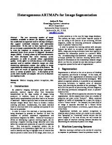
Figure 2.1: Basic regular 2 2=4 pyramid, which can also be seen as a quadtree 2.2.1 Regular Pyramids

The basic idea of regular pyramids is to apply feature detectors at different pyramid levels. One of the first and simplest regular pyramids is the classical 2 2=4-pyramid where every 2 2 pixel block is merged into a single pixel at the level above (fig. 2.1), in the sense that the pixel intensities are averaged to define the intensity of the pixels at higher levels. This merged-into relation can also be seen as the child-of relation of a tree; the 2 2=4-pyramid is therefore often referred to as a quadtree [Sam84]. More generally, in regular pyramids, each pixel of a level l is called the parent of a set of pixels on level l 1, its children. As in the simple 2 2=4-pyramid, their intensities are combined to define the parent’s intensity. However, the children of neighbored pixels can form overlapping sets and the averaging can be weighted in general. Another common regular pyramid is the Gaussian pyramid [Bur84], where each pixel of a level l is assigned a weighted sum of the intensities of several pixels of level l 1, defined by a (Gaussian) kernel. As in the 2 2=4-pyramid, each level is half the size of the one below. Such resolution pyramids turned out to be very shift-dependent, which introduces instability problems if one employs them for image segmentation. [BCR90] gives a thorough description of problems with various published regular pyramid segmentation algorithms from a theoretical and experimental point of view. In fact, shifting the sampling grid by just one pixel may lead to a totally different segmentation result [BCR90]. This local shift-dependency extends to scale- and rotation-variance, since the local effect of small scale changes and rotations by a few degrees corresponds to a local shift. Furthermore, since one of the main features of pyramids is that they convert global image features to local ones and treat local and global aspects of image analysis alike, the approach also suffers from global dependency on scaling and rotation. [BCR90] supports this statement with experimental results. Moreover, the approach of regular pyramids ignores that small details quickly disappear in ascending levels, irrespective of their importance. In some cases, small image features are significant, but there is no way to preserve them in higher levels, so that further interpretation

14

2.2 Hierarchical Segmentation

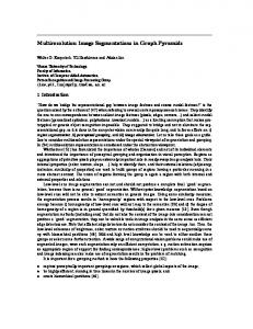
Figure 2.2: This “house” example (as given in [Kro95]) shows that the RAG (black graph in the left drawing) does not contain enough information for the reconstruction of the correct boundary graph, which should be its dual. steps become more difficult. Another motivation for pyramids is parallelization: Pyramids can also be seen as a tapering stack of arrays of “processors” or “cells” (Cellular pyramids, see [MMR91]). Communication happens locally between successive levels (cf. connections in fig. 2.1), which facilitates parallelization for fast multiresolution image analysis [HGS+02]. Many image processing algorithms run on this hierarchical structure in O (log n) parallel processing steps where n is the diameter of the input image [BK01]. It has been shown that the approach of regular pyramids is too rigid for image segmentation [BCR90, MMR91]. This leads to serious problems with disappearing details, or even instability resulting from changes in the sampling configuration. A thorough investigation on shift-, scale- and rotation-variance of five different kinds of regular pyramid has been done by [BCR90]. 2.2.2 Irregular Pyramids

To overcome the drawbacks of regular pyramids, the more general approach of irregular pyramids has been introduced [MMR91]: In order to represent irregular tessellations in which the position of neighbors is not a priori known, each pyramid level is defined by a graph in which each vertex v represents a region in the original image, which is also called the receptive field of v. Thus, the definition of edges between vertices of level l can be done in a straight-forward manner by looking at the adjacency of the corresponding regions - resulting in what is called a region adjacency graph (RAG [Pav77], an example is given in the left image of fig. 2.2). There are several possible definitions of the pyramid’s base, e.g.

considering each pixel a vertex,

15


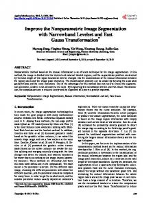
Figure 2.3: Two images which lead to the same RAG (embedded into the plane in two nonhomeomorphic ways).

grouping connected components with the same gray level into the same vertices, or performing a watershed transform on the original image’s gradient magnitude to define the vertices’ receptive fields.

The simplicity of the region adjacency graph becomes apparent if one tries to reconstruct the boundary graph from it. In theory, the dual of the RAG should be isomorph to the boundary graph, but the fact that the RAG does not allow multiple edges leads to problems with boundaries consisting of more than one edge, as for example the wall-background boundary that is separated by the roof and the door. Furthermore, information about disconnected boundary components is lost, which leads to the contour of the window in fig. 2.2 being misleadingly connected to the wall’s contour. Another information of the original image that is not contained in the RAG is in which way the graph should be embedding in the plane. Figure 2.3 contains two different images that lead to exactly the same RAG. 2.2.2.1 Contraction

In order to build higher pyramid levels, parts of the graph are contracted: A contraction is parametrized by the set of survivors and a mapping of each non-survivors to a survivor. Survivors are vertices that are not removed by a contraction but remain in the contracted graph. Each level will be a coarser representation of the image than the level below, in the sense that the corresponding graph will be smaller (has less vertices). In order to have any a vertex correspond to a connected region of the image, the vertices merged into a single parent must form a connected subset of the vertices of level l 1. Edges

16

2.3 Overview of Different Graph Formalisms on level l are defined between vertices which have at least one direct connection between any of their children. The set of survivors and the assignment of non-survivors to them are called contraction parameters. The goal of irregular tessellations is to let higher levels be more abstract representations of the objects while making it possible to preserve details recognized as being significant for a specific task at higher levels. What is left to be defined is the way how the contraction parameters are determined. As a first approach, [MMR91] introduced a stochastic pyramid, which uses a given probability of two neighbors to be of the same class (defined from graylevel similarities for example) in order to iteratively build an irregular sampling hierarchy in log (class_size) parallel steps. In [MMR91], lower and upper bounds are defined for the distance between survivors. The lower bound on the distance translates into a minimum number of non-survivors contracted into them, which results in a lower bound on the reduction factor. Thus, the overall pyramid height and computational costs are also bound. The upper bound on the distance provides locality for implementation with parallelized processors (actually, in [MMR91] only direct neighbors of a survivor are candidates for being contracted into it).

2.3 Overview of Different Graph Formalisms The weaknesses of the graphs mentioned so far are that

they do not contain enough information about the topology to differentiate between the two embeddings of fig. 2.3 and do not allow the reconstruction of the correct boundary graph (fig. 2.2).

This will be improved by substituting the RAG with more complex structures as the ones discussed in the following sections. 2.3.1 Dual Image Graphs

Kropatsch [Kro95] extends the RAG by allowing multiple-edges and self-loops. Multiple edges are used to represent more than one boundary component between two regions, e.g. the wall-background boundary, which is separated into two components by the door and the roof in fig. 2.4. Self-loops represent holes in regions, like the window. Due to the fact that the graphs are no longer required to be simple2 , the resulting two multigraphs are each other’s duals, and Kropatsch calls them dual image graphs. Note that a self-loop leads to a bridge in the dual graph and vice versa, which in contrast to simple region adjacency graphs (RAGs) makes it possible to reconstruct the complete boundary graph: 2 See

section 2.1.1 on page 9 for graph terminology like “simple” and “dual” graphs.

17


Figure 2.4: In contrast to the RAG in fig. 2.2, the dual image graph (DIG) for the house example contains all topological information about its boundary.

Each inner component of the boundary graph (like the window) is surrounded by a self-loop, which results in a new region. That region introduces a node in the dual graph, which was missing in the RAG’s dual (fig. 2.2), which had only one node for two boundary components. Boundaries with more than one component (like the above-mentioned wall-background boundary split into two parts to the left and right of the door) are represented in the extended adjacency graph with double-edges, which lead to the correct number of edges in its dual, the boundary graph.

Note, however, that the window has to be connected to the walls’ outer contour with an auxiliary bridge in the boundary graph. In the dual graph formalism, such connections are mandatory, since disconnected graph components destroy the dualism. The need for auxiliary bridges leads to the following drawbacks of this approach:

18

With this formalism, “real bridges” cannot be represented, since they are indistinguishable from auxiliary bridges. Nevertheless, bridges can result from incomplete segmentations. Since the image segmentation problem requires human intelligence to be solved in general, algorithms often find only parts of an objects’ boundary. It is helpful if a boundary graph can represent the incomplete boundaries with bridges, instead of having no evidence of an object boundary at all. Furthermore, there is no canonical place at which the auxiliary bridge should be attached to the separate boundary components. That makes comparison of segmentation results more complicated, and bridges have to be explicitly ignored by all interpretation steps, since they have no semantic meaning.

2.3 Overview of Different Graph Formalisms

α

=

σ

=

1 10

;

1 50 7

2 20 ;

;:::;

10 70 8 2

30 5 40 ; 6 60 8

8 80 ;

20 3 4

;

Figure 2.5: A combinatorial map encoding the boundary graph of the house example (right of fig. 2.4) In [Kro95], the focus lies on regions and relations between them; as a consequence, bridges always represent disconnected boundary components, and the dual graph contraction operation removes all useless self-loops and bridges. 2.3.2 Combinatorial Maps

A combinatorial map can discriminate between two planar embeddings of a graph which are not homeomorphic by explicitly encoding the order of darts around a vertex. Darts (also called half-edges) are the basic entities of the combinatorial map formalism and can be seen as directed edges (cf. the arrows in fig. 2.5). Definition 2.3.1 (combinatorial map) A combinatorial map is a quadruple (D; σ; α; φ) where D is a set of darts and σ; α; φ are sets of orbits such that each dart belongs to exactly one orbit and all α-orbits have length 2. The orbits in σ; α and φ are called nodes, edges, and faces respectively. A combinatorial map is planar, if it is orientable, that is, if φ (d ) = σ

1

(α (d ))

and if the number of nodes, edges, and faces fulfills Euler’s equation. In its most common form, Euler’s equation states that for a connected boundary set the following holds: n

e+ f

=

n

=

e

=

f

=

2 where

jσj is the number of nodes jαj is the number of edges jφj is the number of faces

(2.1)

19

2 Related Theory and Work For a plane division with any number of connected boundary components, Euler’s equation becomes n

e+ f

k

=

1

where

(2.2)

k is the number of components Definition 2.3.1 of a combinatorial map differs from the original definition [BK00a], which uses permutations of darts instead of sets of orbits (both are equivalent, since permutations define orbits, and orbits can be composed to permutations again). While that definition seems simpler at first sight, it makes subsequent definitions more complicated, since it does not allow empty orbits. These are needed for two special cases:

The trivial map which contains only the infinite face is represented with an empty φ/ φ = f()g orbit. Euler’s equation 2.2 for the case of k = 0 holds with D = σ = α = 0, and the above, straight-forward definitions of n; e and f from (2.1). Empty orbits are used to represent isolated vertices (a vertex is called isolated if no / σ = φ = f()g (it edges are attached to it). The node map is defined by D = α = 0, contains just the infinite face and one isolated node).

Empty orbits allow for a one-to-one correspondence between α-orbits and nodes, σ-orbits and edges, and φ-orbits and faces, respectively. This makes the simple definitions of n; e and f from (2.1) possible. Note that we take the order of darts in a σ-orbit to be that found when turning in mathematically positive direction around the vertex. Without specifying this, a combinatorial map would still allow two non-homeomorphic embeddings (which could be made homeomorphic by mirroring one of them along any axis in the plane). With the extra constraint that a combinatorial map is planar, it can be defined with just a triple (D; σ; α), since φ = σ 1 Æ α. In other words, the φ-orbits (which represent contours of faces) can be composed with a simple contour following algorithm: To get to the next dart which has the same face on its left side, we jump to the opposite dart (α-orbit) and then turn right (σ 1 , the inverse of σ, which turns left). The definitions of composition of permutations and their inverses can easily be transferred onto sets of orbits; the only special case of an empty orbit can be explicitly defined to result in an empty orbit, which will lead to the intended results. As already mentioned, combinatorial maps determine their embedding by the local orientation of the structural elements. Brun and Kropatsch released several publications defining dual contractions (like the previously ones for dual image graphs) on combinatorial maps [BK99a], using the formalism to build irregular pyramids [BK99b, BK00b] and giving sequential and parallel algorithms to implement those pyramids [BK00a]. However, bridges are still needed to connect separate boundary components, so that the disadvantages mentioned in section 2.3.1 still exist. The formalism discussed in the next section will avoid these auxiliary bridges and their drawbacks.

20

2.3 Overview of Different Graph Formalisms 2.3.3 XPMaps

[Köt01, Köt02] introduced XPMaps (eXtended Planar Maps) as an extension of combinatorial maps. XPMaps can explicitly represent regions with holes (such as the window within the wall in fig. 2.2). Definition 2.3.2 (XPMap) An extended planar map (XPMap) is a tuple (C; c0 ; exterior; ontains), where C is a set of non-trivial planar combinatorial maps (the components of the XPMap), c0 is a trivial map that represents the infinite face of the XPMap, exterior is a relation that labels one φ-orbit of each component in C as the exterior orbit, and ontains is a relation that assigns each exterior orbit to exactly one non-exterior φ-orbit or to the empty orbit in c0 . The σ-, α-, and φ-orbits of the components are the nodes, edges, and contours of the XPMap. A face now comprises exactly one non-exterior φ-orbit (outer contour) and the possibly empty set of exterior φ-orbits (inner contours, holes) it contains. In order to construct an XPMap from a given plane division, C has to be built by creating a combinatorial map for each connected component of the division’s boundary set. By definition, c0 is the trivial map. To define exterior for components with more than one φ-orbit, observe that in every component, there must be exactly one φ-orbit that is traversed in mathematically negative direction. This then becomes the exterior orbit. Finally, the relation ontains is constructed according to the inclusion of components within regions of the plane division. Since we will casually speak of “cells” in this work, the connection to the notion of “cell complexes” shall be clarified here. Definition 2.3.3 (cell complex) A cell complex is a triple (Z ; dim; B) where Z is a set of cells, dim is a function that associates a non-negative integer dimension to each cell, and B Z Z is the bounding relation that describes which cells bound other cells. A cell may bound only cells of larger dimension, and the bounding relation must be transitive. If the largest dimension is k, we speak of a k-complex.

Cell complexes were introduced into the field of image analysis by Kovalevsky [Kov89]. Since in image analysis, we want to represent the topological structure of 2-dimensional images, we are interested in 2-complexes whose bounding relation is consistent with a plane division. We call those planar cell complexes, and their 0-, 1-, and 2-cells correspond to vertices, edges, and regions, respectively. Cell complexes are useful if one wants to use topological representations for higher dimensions. XPMaps have only been defined for the 2D case; however they make the exterior and

ontains relations explicit, and cell complexes do not carry information about which contour of a face is the exterior one. [Köt00] proposes the use of cell complexes to represent image segmentation results, which imposes the need for modifying operations which correspond to graph contractions (section 2.2.2.1). The next section will introduce Euler operations on XPMaps, which can be used to create higher levels for irregular pyramids.

21

2 Related Theory and Work (4n, 4e, 4 f , 4k) ( -1 , -1 , 0 , 0 ) ( -1 , -1 , 0 , 0 ) ( 0 , -1 , -1 , 0 ) ( 0 , -1 , 0 , 1 ) ( -1 , 0 , 0 , -1 ) ( 0 , 0 , 0 , 0 )

Operation merge neighbored 0-cells merge neighbored 1-cells merge neighbored 2-cells remove bridge remove isolated 0-cell move component

Inverse split up a 0-cell split up a 1-cell split up a 2-cell add bridge add isolated 0-cell (move component)

Table 2.1: Useful, non-minimal set of Euler operations for image segmentation [Köt00] 2.3.3.1 Euler Operations

Euler operations are operations which hold up Euler’s equation ((2.2)), which has the following form in case of a planar XPMaps (C; c0 ; exterior ; ontains): n

e+ f

k

=

n

=

e

=

f

=

k

=

1

where

∑ jσj is the number of nodes

(2.3)

c2C

∑ jαj is the number of edges

c2C

!

∑ jφj

j j

(C

c2C

1) is the number of faces

jCj is the number of connected boundary components

Equation 2.3 can be interpreted as a hyperplane equation in a four-dimensional parameter space: > (1; 1; 1; 1) (n; e; f ; k) = 1 Each modifying operation has an associated parameter change vector

4n 4e 4 f 4k)

(

;

;

;

where its entries represent the changes of the parameters n; e; f ; and k. The parameter change vector must be parallel to the hyperplane in order to obey equation (2.3), that means (1;

1; 1; 1) (4n; 4e; 4 f ; 4k)> = 0

must hold. In a four-dimensional space, three independent basis vectors are enough to span a hyperplane. Therefore three operations and their inverse provide a minimal, complete set to transform any XPMap into any other. However, one usually employs some more operations to allow for more concise and clear formulations of algorithms. [Köt00] mentions a total of five operations plus their inverses to be especially useful in the context of image segmentation with cell complexes, see table 2.1.

22

2.4 Region Representations

2.4 Region Representations The purpose of image segmentation algorithms is a tessellation of the image into disjoint regions and boundaries between them. The segmentation result can be represented on different levels [Köt00]: Iconic representations are commonly used and known as “labelled images”: A unique la-

bel is assigned to each region, and the segmentation of an image Iorig is stored in a second image Ilabels of the same size, in which each pixel value is the label of the region associated with that pixel position. Geometrical representations represent objects (or parts of them) with geometrical models

the parameters of which are adjusted after measurings in one or more images. Topological representations stress the topological structure (bounding-relations / adjacen-

cies) of the regions. Normally, purely topological representations as introduced in 2.3 are not sufficient for further image analysis steps, but some geometrical properties are needed, which leads to combinations with other representations. 2.4.1 Iconic Representations

In this section, we will compare the following iconic representations: Boundaries on pixels, which can be 8-connected as in this image, implying 4-connected regions to prevent the connectivity paradox, or vice versa.

Crack-edge boundaries between pixels of an image plane which is completely labelled into touching regions.

Crack-edges made explicit as newly-inserted crack-edge rows (/columns) between every two rows and columns of the original region image.

Boundaries on the hexagonal pixels of a region image sampled with a hexagonal raster.

23


Figure 2.6: The connectivity paradox (see text) 2.4.1.1 Connectivity

In the common square grid of an image, there are two different connectivity definitions: Definition 2.4.1 (4-connectivity) Each pixel is considered to be 4-connected with its four direct neighbors. Definition 2.4.2 (8-connectivity) A pixel is 8-connected with its four direct and its four indirect neighbors, which are diagonally adjacent. The fact that there is a difference between direct and indirect neighbors leads to the connectivity paradox, which can be explained by means of fig. 2.6. Here, the Jordan Curve Theorem is violated if one uses either 4-connectivity or 8-connectivity for both the curve- (black) and the region pixels (white): Theorem 2.4.1 (Jordan Curve Theorem) Any continuous simple closed curve in the plane separates the plane into two disjoint regions, the inside and the outside. If we choose 8-connectivity, the curve is closed but the inner region and the outer region are still connected. With 4-connected pixels, there are two regions, but the curve is not closed anymore. There are different possible solutions to this problem, which are described in the following paragraphs. 2.4.1.2 Boundaries on Pixels

The first type of iconic region representations arises if not every pixel is assigned a region label, but the regions are separated by explicitly represented boundary pixels. This can be the result of some implementations of the watershed algorithm [VS91, RM00] that leave watersheds unlabelled. Also, Canny’s edgel linking from [Can86] will connect pixels marked as edge pixels into boundaries. To prevent the connectivity paradox, one can use 8-connectivity for the foreground (the curve) and 4-connectivity for the regions, which leads to a closed curve and two regions in fig. 2.6. Defining it the other way round (resulting in one region and an open curve) does

24


11 00 00 11 00 11 00 11 00 11

11 00 00 11 00 11 00 11 00 11

Figure 2.7: Two non-thin example sections of 8-connected boundaries solve the problem, too, but is not done as often because the before-mentioned definition does obviously better fit the human perception. The definition of connectivity becomes very important since we want the regions to be separated - thus there must not be a “gap” in the boundary. On the other hand, we want the boundary to be “thin”, i.e. it should not contain unnecessarily many pixels. This will be made explicit by definition 2.4.3. Definition 2.4.3 (thin boundaries) In an iconic representation of regions and boundaries, a boundary is defined as being thin, if no pixel can be removed from it without changing the connectivity of the surrounding regions. 8-connected boundaries can be made non-thin by adding single pixels in such a way that they still “look thin”, see the marked pixels in fig. 2.7. The T-junction to the left is a very common case, which is sometimes desirable to be retained in spite of the basic requirement towards the rest of the boundary to be thin. Figure 2.7 illustrates that requiring an 8-connected boundary to be thin according to definition 2.4.3 is a rather strong requirement. Section 4.6 discusses this in more detail, and section 4.6.1 deals with the T-junctions in particular. 2.4.1.3 Crack Edges

Another solution for the connectivity paradox are crack-edge representations, where we assign each pixel a region label (i.e. there are no boundary pixels in the image) and define edges as lying between the pixels of two different regions. This is a fundamental difference compared with the other kinds of region representations, since contours exist implicitly where two regions touch, which leads to fundamental changes in reasoning algorithms (compared to boundaries on pixels). For example, the output of an edge detection operator (like the Gaussian gradient) is normally represented in an image of the same size as the original image, and the gradient value on an edge is not directly accessible but must be interpolated from the adjacent pixels. ([Köt03c] shows that in order to use Gaussian gradient kernels with small scales which preserve fine details, storing the result in an image of the same size violates Shannon’s law. Thus, Köthe proposes an oversampling gradient algorithm which provides reasonable gradient values for crack coordinates in a natural way.)

25


Figure 2.8: The creation of an explicit crack edge representation by crack insertion 2.4.1.4 Explicit Crack Edges

This is a combination of both of the above representations, since the boundary is on pixels, but only on crack coordinates: Between each two columns (rows) of the region image, an extra crack-edge column (row) is inserted, nearly-doubling the image size from w h to (2w 1) (2h 1). Given a w h region image Ilabels as input, the explicit crack edge image Icracks can be derived with the following algorithm: 1. Create an image of size (2 w

1) (2 h

1). Copy each label Ilabels (x; y) into Icracks (2 x; 2 y).

2. Fill missing pixels in the even columns: For each position (x; y) with an odd y and an even x in Icracks , a) if Ilabels (x=2; y=2) = Ilabels (x=2; y=2 + 1), copy this label into Icracks (x; y), b) otherwise mark this cell with a special boundary label 3. Fill odd columns: For each position (x; y) with an odd x in Icracks , a) if Ilabels (x=2; y=2) = Ilabels (x=2 + 1; y=2), copy this label into Icracks (x; y), b) otherwise mark this cell with a special boundary label The process is illustrated in 2.8. Ilabels is assumed to be the result of a segmentation algorithm, but without boundary pixels, i.e. all pixels should have been assigned a region label. The result of this algorithm can also be expressed as 8 Ilabels (x=2; y=2) > > > > Ilabels ((x)=2; y 1=2) > >
> > > > > :

Icracks (x

if x and y are even if x is even, y is odd and Ilabels ((x)=2; y 1=2) = Ilabels ((x)=2; y+1=2) 1; y) if x is odd and Icracks (x 1; y) = Icracks (x + 1; y) b else

where 0 x < w and 0 y < h and b is the special crack-edge boundary label.

26


Figure 2.9: A Khalimsky plane The resulting crack-edge image allows both 4- or 8-connectivity to be used for the region or boundary pixels, because in effect, both the boundary and the regions consist of 4-connected pixels and problematic cases as in fig. 2.6 cannot occur anymore. There is a strong relation between such crack edge images and the Khalimsky plane [KKM90]. Definition 2.4.4 (Khalimsky plane) A Khalimsky plane is defined on Z2 by denoting points with two even coordinates as faces, points with two odd coordinates as nodes, and mixed points as edges. Nodes bound their eight neighbors (four edges and four faces), and edges bound the two neighboring faces. Thus, Khalimsky planes are cell complexes (definition 2.3.3) with a regular structure, as illustrated in fig. 2.9. Their structure is very similar to that of crack edge representations, since cells with two even coordinates are faces(compared to region pixels), nodes have two odd coordinates, and edges mixed odd and even ones. However, the Khalimsky grid has a rigid structure in which every cell with an odd coordinate is a node or edges, whereas these are only candidates for boundary pixels in a crack-edge representation that is adopted to the content (the labelled regions). At the same time, the structure of explicit crack edge images is very similar: Each pixel with two even coordinates is a region pixel, and the boundary is in between. In Khalimsky grids however, each cell with at least one odd coordinate is an edge or a node, whereas this depends on the uniformity of the regions in crack edge images. It is possible to define cell complexes on top of other cell complexes. [Köt00] describes how a cell complex can be based on a Khalimsky plane 2.4.1.5 Hexagonal Grid

The idea of sampling images with a hexagonal grid instead of a square one goes back to Golay [Gol69], and further research on its application in the field of computer vision was done by Overington [Ove92] starting in the seventies. A key motivation is that hexagonally sampled images are supposed to reduce the computational cost of image analysis. Since each pixel has

27

2 Related Theory and Work six equivalent neighbors, there is no connectivity paradox, and many algorithms benefit from the fact that they do not have to deal with the different types of neighborhoods which exist in a square grid. Overington claimed hexagonal grids to be superior with respect to edge detection performance. Nevertheless, in experiments with edge detection operators on graylevel-images [BBH02], the results have been similar to the ones using square grids. Overington also applied the formalism to colored motion scenes and stereo vision with and without noise, but the results of [BBH02] for the basic case of static graylevel images imply that modern approaches using square grids might be equally accurate in those cases, too. However, the question whether the greater regularity of hexagonal grids makes faster implementations of algorithms possible is more difficult to address, and still remains to be answered. Experiments with hexagonal grids for the basic representations go beyond the scope of this work, but we will casually refer to hexagonal grids from a theoretical point of view. 2.4.2 Deriving Topological Representations from Pixel Boundaries

Depending on the type of region representation, it can be difficult to derive a correct topological structure from that region image. So far, we discussed several region representations and the implied definitions of boundaries between them. If we want to use iconic region representations as the basis for topological structures like XPMaps, we have to define how the boundary is split into nodes and edges. The definition of faces is straight-forward; a face can be defined as a connected set of region pixels with the same label. Per definition, to constitute a topologically correct XPMap, we have to make sure that no two nodes, edges, or faces are directly adjacent. This can be achieved by appropriate definitions of the concrete representation of nodes and edges and their neighborhoods.

Faces must be bound by edges and nodes (which has already been ensured in section 2.4) Edges must be bound by two nodes (or one, in case of a self-loop), and it must be possible to derive the α-orbits. For each node, we need to define its σ-orbit. This means, we do not only need the node’s degree, but also the order in which edges are met while turning anti-clockwise around the node.

Furthermore, we need a representation of darts - the fundamental entities used in the definition of XPMaps (resp. combinatorial maps, definition 2.3.1 and 2.3.2). A dart (half-edge) can be represented based on the representations of nodes and edges; note however that it is not welldefined in all cases by just specifying the starting node and the edge it points to, since there are two opposite darts for each self-loop. In section 3.4 we describe our dart representation which is basically a pair of a node pixel position and the direction it points to.

28


Figure 2.10: Building an XPMap based on a Khalimsky plane The following sections will describe how correct topological information can be extracted from the region representations discussed in the last section. 2.4.2.1 Crack-edge boundaries

Separating the boundary into nodes and edges is most easily done on a crack-edge representation, which is one of the reasons why those representations became popular. Vertices in a crack-edge boundary comprise exactly one pixel and have a maximum degree of four (cf. the Khalimsky grid, definition 2.4.4). Candidates for node pixels are exactly those pixels which have four region pixels as diagonal neighbors. The simplest approach is to mark all node pixel candidates on the contour as nodes, but that leads to a great number of nodes and edges. Actually only nodes with degree > 2 are needed, with one exception: A boundary component is allowed to consist of only one closed loop. Somewhere on such a loop, a node has to be inserted to make the structure topologically correct. A possible way to obtain a correct crack-edge based XPMap representation is to begin with a Khalimsky plane built by Crack Insertion as in fig. 2.10. The Crack Insertion algorithm has been described in section 2.4.1.4 for crack images; [Köt03a] presents the same algorithm for Khalimsky planes. Then, the “merge edges” Euler operation can be used to merge all unneeded nodes into their surrounding two edges to get a longer edge. Similarly, all faces, edge, and nodes of the Khalimsky plane which carry the same region label can be merged into a single region of the XPMap. 2.4.2.2 8-Connected Boundaries on Pixels

In section 2.4 we mentioned the common representation of segmentation results as 8-connected boundaries on a 4-connected background (or vice versa, as discussed in section 2.4.2.3). Köthe [Köt03a] seems to be the first to publish a non-heuristic way to classify and link such boundary pixels into nodes and edges. The following definition of the difference between node- and edge-pixels is given in [Köt03a]:

29

2 Related Theory and Work Definition 2.4.5 (boundary pixel classification) A boundary pixel in a thin boundary image is classified as an edge pixel if its 8-neighborhood consists of exactly four 4-connected components, and neither of the components consisting of boundary pixels contains more than one 4-neighbor.3 Otherwise, the pixel is a node pixel. (If configuration 5 is allowed, it is treated exceptionally and marked as a node pixel as well.) The number of possible configurations is given as 28 = 256 since each of the eight neighbors of a boundary pixel may either belong to the boundary or to the background. After filtering out configurations which can be derived from others by rotation or reflection, 51 unique configurations remain which are listed in table 2.2 on the next page

3 “4-neighbor”

30

is meant as a 4-neighbor of the center pixel here.

2.4 Region Representations .

11 00 00 11 00 11 1A 00 11 00 11 00 11 00 11 00 11 00 11 node pixel 00 11 00 11 00 11 00 11 00 11 00 11 0011 11 0011 00 or reducible 1111 00 0011 00 00 11 00 00 0011 11 0011 11 00 11 0011 11 0011 11 00 11 00 11 00 00 00 11 00 11 00 0011 11 0011 00 11 0011 11 0011 11 00 11 00 11 00 00 00 11 00 11 00 0011 11 0011 00 11 0011 11 0011 00

0011 11 0011 00 11 00 00 11 00 11 00 11 00 11 00 11 00 11 00 00 0011 11 0011 11 00 11 00 11 00 11 00 11 00 11 00 11 00 11 00 11 00 11 00 0011 11 0011 00 11 00 11 00 11 00 0011 11 0011 00 11 0011 11 0011 00

4B cannot occur (not thin)

11 00 00 11 00 11 00 11 00 11 00 11 00 11 00 11 00 11 00 11 00 11 00 11 00 11 00 11 00 0011 11 0011 00 11 00 11 00 11 00 11 00 11 00 11 00 11 00 11 00 11 00 11 00 11 00 11 00 11 00 11 00 11 00 0011 11 0011 00 11

2A node pixel or reducible

11 00 00 11 00 11 3A 00 11 00 11 00 11 00 11 00 11 00 11 node pixel 00 11 00 11 00 11 00 11 00 11 00 11 0011 11 0011 00 or reducible

5A corner (see text)

6 edge pixel

7 edge pixel

8 edge pixel

9 edge pixel


11 edge pixel

12 edge pixel

13 edge pixel

11 00 00 11 00 11 00 11 00 11 00 11 00 11 00 00 0011 11 0011 11 00 11 00 11 00 11 00 11 00 11 00 11 00 11 00 11 00 11 00 0011 11 0011 11 00 11 00 11 00 00 11 00 11 00 11 00 11 00 11 00 11 00 0011 11 0011 00 11

A 11 00 00 00 0011 11 0011 11 00 16 11 00 11 00 00 0011 11 0011 11 00 T-config 11 00 11 00 11 00 0011 11 0011 00 (see text) 11

19 node pixel


11 00 00 11 00 11 00 11 00 11 00 11 00 11 00 00 0011 11 0011 11 00 11 00 11 00 11 00 11 00 11 00 11 00 11 00 11 00 11 00 0011 11 0011 11 00 11 00 11 00 00 11 00 11 00 11 00 11 00 11 00 11 00 0011 11 0011 00 11

17 node pixel 1111 00 0011 00 00 11 00 00 0011 11 0011 11 00 11 00 11 00 00 0011 11 0011 11 00 11 00 11 00 11 00 0011 11 0011 11 00 11 00 11 00 00 0011 11 0011 00 11 00 11 00 11 00 0011 11 0011 11 00 11 00 11 00 00 11


15B cannot occur (not thin) 18 node pixel

A 11 00 00 00 0011 11 0011 11 00 21 11 00 11 00 00 0011 11 0011 11 00 node pixel 11 00 11 00 11 00 0011 11 0011 00 or reducible 11

22 node pixel

23 edge pixel

24 edge pixel

25 edge pixel

26 node pixel

27 node pixel

28 edge pixel 31 node pixel

11 00 00 11 00 11 34A 00 11 00 11 00 11 00 11 00 11 00 11 node pixel 00 11 00 11 00 11 00 11 00 11 00 11 0011 11 0011 00 or reducible

11 00 00 11 00 11 29A 00 11 00 11 00 11 00 11 00 11 00 11 node pixel 00 11 00 11 00 11 00 11 00 11 00 0011 11 0011 00 or reducible 11

11 00 00 00 0011 11 0011 11 00 11 00 11 00 11 00 11 00 11 00 11 00 11 00 11 00 11 00 0011 11 0011 11 00 11 00 11 00 00 11 00 11 00 11 00 11 00 11 00 11 00 0011 11 0011 11 00 11 00 11 00 00 0011 11 0011 00 11


32 node pixel

0011 11 0011 11 00 11 11 00 00 00 00 11 00 11 00 11 00 11 00 00 0011 11 0011 11 00 11 00 11 00 11 00 11 00 11 00 11 00 11 00 11 00 11 00 0011 11 0011 11 00 11 00 11 00 00 11 00 11 00 11 00 0011 11 0011 00 11


35 edge pixel

11 00 00 11 00 11 00 11 00 00 0011 11 0011 11 00 11 00 11 00 11 00 11 00 11 00 11 00 11 00 11 00 11 00 0011 11 0011 11 00 11 00 11 00 00 11 00 11 00 11 00 11 00 11 00 11 00 11 00 11 00 11 00 0011 11 0011 00 11


31


0011 11 0011 00 11 00 00 11 00 11 00 11 00 11 00 11 00 11 00 00 0011 11 0011 11 00 11 00 11 00 11 00 0011 11 0011 00 11 00 11 00 11 00 0011 11 0011 00 11 00 11 00 11 00 0011 11 0011 00 11 0011 11 0011 00

1111 00 0011 00 00 11 00 00 0011 11 0011 11 00 11 00 11 00 00 0011 11 0011 11 00 11 00 11 00 11 00 0011 11 0011 11 00 11 00 11 00 00 11 00 11 00 11 00 11 00 11 00 11 00 0011 11 0011 11 00 11 00 11 00 00 11

37 node pixel

1111 00 0011 00 00 11 00 00 0011 11 0011 11 00 11 00 11 00 00 0011 11 0011 11 00 11 00 11 00 11 00 0011 11 0011 11 00 11 00 11 00 00 0011 11 0011 00 11 00 11 00 11 00 0011 11 0011 00 11 0011 11 0011 00


39 node pixel

40 node pixel

1111 00 0011 00 0011 11 0011 11 00 11 00 11 00 00 00 11 00 00 0011 11 0011 11 00 11 0011 11 0011 11 00 11 00 11 00 00 00 11 00 11 00 0011 11 0011 00 11 0011 11 0011 11 00 11 00 11 00 00 0011 11 0011 00


42 node pixel 0011 11 0011 00 11 00 00 11 00 11 00 11 00 11 00 11 00 11 00 00 0011 11 0011 11 00 11 00 11 00 11 00 0011 11 0011 00 11 00 11 00 11 00 0011 11 0011 00 11 00 11 00 11 00 0011 11 0011 00 11 0011 11 0011 00


44 node pixel


46 edge pixel

47 node pixel

48 node pixel


50 node pixel

51 node pixel

Table 2.2: The 51 unique 8-neighborhood configurations of a boundary pixel, and their classification. Patterns marked with hatching do not occur in thin boundaries, see text. Configurations marked with a “B” and 30Æ right-diagonal hatching cannot occur in a thin boundary. Configurations with an “A” and 45Æ left-diagonal hatching are reducible in a strict sense, but those configurations are often desirable, and can be generated by an appropriately modified thinning algorithm:

32

Configuration 5 is the 90Æ corner configuration. In axes-parallel rectangles, removal of those points would make its corners look “round”. According to [Köt03a], this pattern should be classified as a node pixel, too. Configuration 16 is the T-junction. As discussed in section 4.6.1, removal of the center pixel leads to displaced pixels in straight lines - which is especially annoying because this is often caused by unwanted “streamers”. Configurations 2 and 3 mark the end of a dangling edge. Often, low contrast leads to gaps in a contour, which can later be repaired by higher level analysis and perceptional grouping. In section 2.3.3, we made sure that our theoretical framework is able to cope with such bridges, and now it should be clear that we do not want to lose them while thinning. Therefore, we use a modified thinning algorithm and classify those end-point configurations as node pixels.


Figure 2.11: Classification of Vertex pixels according to Tieck and Gerloff [TG97] (original image from there) Note that our experimental work with 4-connected boundaries has shown that in general, the classification scheme described here still is applicable, but configuration 5 should be classified as an edge pixel due to the staircase effect which 4-connected diagonal lines suffer from. 2.4.2.3 The Approach of Tieck and Gerloff

[TG97] defined a way to classify 4-connected boundary pixels into edge- and node-pixels; however, their approach differs from the one described in this work in several respects:

Their vertices consist of only one pixel each. To create topologically sound structures, they needed to introduce virtual edges and virtual regions between vertex pixels (see fig. 2.11). Those cannot be represented in the label image, but have to be stored separately in graph-like data structures. In contrast to that, our CellImage is a complete representation and allows the reconstruction of the XPMap and all meta-information. Their data structure consists of a RAG and a watershed graph (WSG).

33

2 Related Theory and Work The RAG is required to be simple, such that their approach is not able to represent multiple boundaries between two regions, or even bridges in case of incomplete boundaries. (See section 2.3 for a thorough analysis.) The WSG is represented with a labelled image similar to our cell image (cf. section 3.4). To retain the duality of both graphs (in particular the bijection between both edge-sets) [TG97] needed to introduce a mandatory second merging step if the resulting WSG has vertices with degree two.

Virtual edges and regions make merging regions much more complicated, because only a subset of the represented edges is removable; the merging procedure has to detect if – the resulting region would still be 8-connected and – the contour in the WSG would remain thin. The first problem is caused by the existence of null-edges, which can be avoided by allowing vertices consisting of more than one pixel. The latter problem has also shown up in our work, when big nodes are merged into the surrounding edges. It can be solved with additional thinning steps, as described in section 4.6.2.

The detection of non-removable edges is done as part of the merging algorithm which greatly increases its complexity. To construct and test their system, they tried to come up with a complete set of basic patterns of merge situations. Although they describe several approaches of searching for such a set, they could not show that the presented set of 21 basic cases was complete.

The author believes that the fact that this search failed shows that the approach has been too complicated. In our approach, the single region merge operation described in [TG97] is equivalent to a sequence of Euler operations: 1. a merge faces operation possible followed by a number of remove bridge operations to remove all edges of the common boundary 2. a sequence of merge edges-operations to remove any node of degree two in the resulting boundary (A complete region merge algorithm on top of our abstract data type will be described in context of the Interactive Paintbrush tool in section 3.2.3.) The fact that an XPMap (even a combinatorial map) combines the information content of the two separate dual graphs reduces the complexity of Euler operations modifying it. Each Euler operation has explicit preconditions that define when and where it is applicable and postconditions that determine in which way the topology has been altered.

34

3 The G EO M AP Abstract Data Type This chapter introduces an abstract data type (ADT) which we call G EO M AP and which is intended as a unified representation for segmentation results. After describing some preliminaries, we will analyse the requirements posed by segmentation algorithms towards such a representation in section 3.2. Subsequently, we will take these requirements into account in the discussion of our interface design of the G EO M AP and the associated helper types (section 3.3). In section 3.4, we will propose an internal “cell image” representation for the GeoMap ADT. Finally, an appropriate interface for a pyramidal data structure based on G E O M APs is discussed in section 3.5.

3.1 Preliminaries 3.1.1 Cell Regions

In our work, all three types of cells can be associated with any number of pixels in the segmented image. In conventional irregular pyramids, every node of a layer’s graph represents a connected set of pixels in the original image (cf. section 2.2.2), such that the complete set of nodes defines its segmentation into regions. In our XPMap pyramids, we have nodes, edges, and faces and - depending on the iconic representation - they correspond to different features in the original image:

Figure 3.1: Vertices with more than one pixel

35

3 The G EO M AP Abstract Data Type

In implicit crack-edge representations, boundaries are located between pixels, so edges correspond to a connected path of pixel-sides and vertices are at the corner points between four pixels. With 8-connected pixel boundaries, edges are thin 8-connected sets of pixels in which each pixel must have a successor and a predecessor. All pixels of a thin boundary which do not fulfill this requirement have to be classified as vertex pixels. Nodes are represented by an 8-connected set of such vertex pixels, where the number of pixels “grows” with increasing degree1 , see fig. 3.1 (section 4.6.2 discusses problems that can arise from this).

In general, we will always think of all cell types (including vertices in particular) consisting of any number of pixels in the following. 3.1.2 Cell Labels

As section 3.4 will explain in detail, our cells carry identifying labels. In the following subsections, “labels” will refer to natural numbers which are at least guaranteed to be unique per cell type. We will not require them to be consecutive or unique for all cells, i.e. an edge and a node might both carry the same label. 3.1.3 I MAGE T RAVERSER

An I MAGE T RAVERSER is a basic concept of the VIGRA image processing library [Köt03d] and represents a position in an image. It is important to understand the implications of its generic nature on the efficiency of the part of our ADT’s interface responsible for accessing the geometry. The coordinates are stored and accessible separately for each dimension in an I MAGE T RA VERSER, which makes it different from a simple memory pointer. Possible commands include “increase the X-coordinate by one” to move to the right in the image, or “set the Y-coordinate of a to the Y-coordinate of b” if two I MAGE T RAVERSERs a; b are available. The importance of the I MAGE T RAVERSER can only be made clear in the context of the VIGRA library: VIGRA stands for “Vision with Generic Algorithms” and exploits the C++ language features of template-functions and -classes to offer generic algorithms on a very high level of abstraction. In contrast to other image processing libraries, VIGRA algorithms do not work on specific images (like graylevel, or RGB images with a fixed bit depth and memory layout), but can work on any image data type for which I MAGE T RAVERSERs exist. Actually, the upper left- and lower right-traversers typically given to algorithms do not even have to represent the upper left and lower right corner of images. It is possible to process subranges 1 [TG97]

introduced “virtual edges” and “virtual regions” between the vertex pixels, which assured that every vertex always consists of exactly one pixel but made the formalism more complicated than necessary, as discussed in section 2.4.2.3.

36

3.2 Requirements of Segmentation Algorithms of images as well as to use I MAGE T RAVERSERs that do not even correspond to positions in real images but perform additional calculations (like interpolations) on demand. To achieve this high flexibility, any object can be used as an ImageTraverser if its interface fulfills the following requirements (exact definitions can be found in the VIGRA documentation [Köt03d] or in [Köt00, section 4.2, table 2]):

It must give access to each coordinate (e.g. x and y for a typical 2D image traverser). It allows dereferencing, i.e. it is possible to access the pixel the I MAGE T RAVERSER currently points to. It must contain type definitions, such that an algorithm can for example determine what the pixel type is which is returned by dereferencing.

The outcome of this concept is that the same algorithms can be used on images with 8- or 32bit graylevels, floating-point values (e.g. used for filtered images), and different colorspaces. I MAGE T RAVERSERs are important for the definition of our ADT, because they allow for a very flexible but lean interface for querying the geometry of cells.

3.2 Requirements of Segmentation Algorithms In this chapter we will have a look at different segmentation algorithms and what kind of operations they are based on. This will allow us to design the G EO M AP ADT in a way that helps making the algorithms more concise, comprehensible, comparable and combinable.

3.2.1 Canny Edge Detection

Canny [Can86] describes an edge detection approach consisting of several steps which are representative for similar steps in many modern image segmentation approaches. The core2 of Canny’s edge detector performs the following steps: 1. Application of an Edge Detection Operator: At first, the original image is inspection with an edge detection operator which indicates the local “edgeness” at each position. After theoretically deriving the optimal edge operator, Canny shows that its shape is very similar to the gradient of a Gaussian. Since the Gaussian gradient has several properties that make it computationally attractive (for example, the 2-dimensional kernels are separable), it is the most common edge detection operator to date. 2 We

left out the application of this procedure in multiple scales, which is not relevant in this context.

37


Figure 3.2: Canny’s edge detection approach provides sub-pixel accuracy but fails near junctions and corners due to problems with the Gaussian gradient.

38

3.2 Requirements of Segmentation Algorithms 2. Non-Maxima Suppression: The result of step 1 is an image containing an edgeness value for each pixel position, but the goal is to find edges. Those are supposed to be indicated by local maxima in this image. Canny filters the gradient image by searching for pixel positions at which the gradient magnitude is a local maximum along a straight line in direction of the gradient. There are other kinds of non-maxima suppression; compared to the common watershed algorithm which is used in our work, Canny’s non-maxima suppression produces “edgels” with a better quality in general, but has the disadvantage that it does not naturally produce closed boundaries. 3. Edgel Linking: The procedure from [Can86] then uses a heuristic method to link independently found edgels into edges. Edgel linking is an important step since we are looking for the boundaries of the 2-dimensional projections of objects. However, coping with any set of edgels resulting from the non-maxima suppression described above is a difficult task, since no assumptions can be made about the properties of the edgels found. Another common approach of edgel linking is to simply search for the “next” pixel in the neighborhood of an edgel, following an edge pixel-by-pixel. However, [Köt03a] seems to be the first to publish an algorithm for transforming an image with boundary pixels into a topological representation without resorting to heuristics. This concrete solution for the specific case of 8-connected boundaries plays an important role in this work:

In [Köt03a], an algorithm is defined which gets a boundary image as input (in which each pixel is either classified as region- or boundary-pixel) and produces a classification of each boundary pixel as either a vertex-, or an edge-pixel. Requiring the boundary to be “thin”, Köthe gives a well-defined way to link 8connected edge pixels into edges, which he was able to prove to be topologically correct.

We use this definition to build a “cell image”, which contains all information necessary to serve as an XPMap representation. In section 3.4, this is explained in detail, and we will show how exactly the XPMap’s orbits are represented and can be retrieved or modified. The classification proposed by [Köt03a] is described in more detail in section 2.4.2.2, and section 4.6 deals with thinning of 8-connected boundaries. 4. Hysteresis Thresholding: After linking edgels together, the result is again filtered in [Can86] (i.e. the number of edges is reduced); hysteresis is used so that lines that include strong and weak gradients are not split up. Two thresholds t1 and t2 for the gradient magnitude are introduced, with t1 < t2 . For a given edge pixel, if the gradient magnitude is below t1 , it is unconditionally removed. On the other hand, edgels with a gradient greater than t2 are considered significant in always remain. Finally, all edge pixels with a magnitude between t1 and t2 are only kept if they belong to an edgel chain which has at least one point with a significant magnitude (> t2 ).

39

3 The G EO M AP Abstract Data Type In other words, after thresholding with t1 , the edges from step 2 are filtered by keeping only those which have at least one pixel which would also survive thresholding with t2 . Canny’s edge detection approach is a good example illustrating the subtasks of image segmentation: 1. Filtering the image to collect evidence for boundaries 2. Non-maxima suppression to get a first set of boundaries 3. Removing insignificant edges from this first boundary set being an oversegmentation This is exactly the approach used in irregular pyramid approaches - the bottommost level is initialized with a graph representing the oversegmentation and further levels are derived by contracting this graph. The contraction parameters are defined according to a cost measure which corresponds to a specific boundary significance measure. For example, the Canny hysteresis thresholding corresponds to an edge significance measure based on the gradient pixels associated with an edge. However, that is only one possible definition; in section 4.4 we will describe other edge- and region-based measures, and perceptual grouping could be used to exclude edges from filtering which are plausible continuations of each other. The XPMap formalism facilitates abstracting from the concrete cost definition, by providing the natural basal elements for such definitions: edges and boundaries consisting of several edges, which will make the hysteresis thresholding algorithm easy to formulate. In addition, it gives direct access to the regions bound by an edge, and any meta-information associated with them (like gray-level histograms) can be used to rate the significance of an edge. In order to support such significance filtering, we need a way of querying the geometry of an edge in such a way that it can be mapped on gradient images for example. Finally, Euler operations will be useful for removing the filtered edges. 3.2.2 Seeded Region Growing

Seeded region growing is a very popular algorithm, or maybe class of algorithms, since besides the original algorithm [AB94] there are many variants. As the name says, it starts with seeds which grow into the final regions. The basic procedure which is similar across all region growing variants is the following: 1. The region growing process is initialized by putting seeds at certain positions. The number of seeds pre-determines the number of regions in the final result. 2. Each seed is given a unique region label in a work image, the rest of this image is marked “unlabelled”.

40

3.2 Requirements of Segmentation Algorithms 3. The neighbors of each pixel that carries a region label l are candidates for growing. Each candidate pixel is associated a certain cost for merging into the region l and put into a queue sorted by this cost. 4. The candidate with the lowest cost is taken from the queue. If the candidate pixel has not been labelled yet (it could have been labelled in the meantime because it was candidate for another region with a lower cost) it is labelled with the region label and its unlabelled neighbors are put into the queue (loop to step 3). If no more candidates are in the queue in step 4, the algorithm terminates with a complete tessellation of the image (each pixel is associated a region label). However, there are other possible conditions for earlier termination, for example an upper bound on the cost, a percentage of pixels that shall be labelled, or the requirement to keep pixel borders between regions. A concrete example of a region growing instance is the watershed algorithm3 from [VS91]. The watershed transform starts with deriving a gradient image from the source image to be segmented. The purpose of the transform is to let the boundaries between regions lie on local maxima of the gradient magnitude. To calculate watersheds, step 1 puts a seed into each local minimum of the gradient magnitude image. The cost for associating a pixel with a region is simply the pixel’s gradient magnitude value, independently of the region. In a complete tessellations, the watersheds lie between labelled regions, i.e. on crack edges (cf. section 2.4). The algorithm can be slightly modified by labelling pixels which are candidates for more than one region with a special “watershed” label to get pixel boundaries in the image. There are two relations between seeded region growing algorithms and our work: 1. The result of a region growing algorithm can serve as the initial segmentation for the pyramid’s bottommost level. As presented in chapter 4, we used a watershed transform in our experiments. 2. Furthermore, a similar region growing can be implemented on top of a G EO M AP: Some regions can be marked as seed regions, and their neighbored regions can be considered candidates for merging. This imposes the following interface requirements: a) If the seeds are manually selected, a mapping from mouse pointer to region must be possible. b) The neighbors of a region must be retrieved to make them candidates; this information is contained in the XPMap (see also section 3.2.5). c) Associating a candidate pixel with a region corresponds to merging a whole region into an adjacent one. On XPMaps, this is done with the “merge faces” Euler operation. Again, a cost measure is needed for the region growing, this time representing the significance of the complete boundary between two regions (which might consist of more than one edge). 3 This

original variant of the watershed transform calculates watersheds “by immersion”, see [RM00].

41

3 The G EO M AP Abstract Data Type 3.2.3 Interactive Paintbrush

This tool for interactive image segmentation introduced by F. Maes in [Mae98] enables the operator to “paint” over region boundaries to initiate region merge operations. Again, this can be seen as a kind of significance filtering - this time the significance is defined by the user’s intelligence instead of formally. The following needs arise towards our data structure:

The algorithm needs to be able to determine the region the operator clicked into or moved into with the (mouse) pointer. When moving the mouse into a new region, it has to decide whether the regions have a boundary in common4 , in which case they should be merged. The Interactive Paintbrush needs to merge regions, which will also be an operation available in our G EO M AP abstract data type. Furthermore, conventional implementations based on labelled region images show that merging should be done in an intelligent way to be efficient: Since this tool results in large numbers of small regions to be merged into one, which will effectively grow until it is much larger than the other regions, it is advisable to always re-label the smaller one of the regions. To do this, one can make use of meta-information on the regions, like the bounding box. This meta-information will also be used and made available by our G EO M AP implementation. When using the Interactive Paintbrush, the regions are commonly displayed with their average color. It will be useful to have the possibility to associate this applicationspecific meta-information with the faces.

3.2.4 Intelligent Scissors

This interactive tool has been introduced in [MB95] and enhanced in [MB98, MB99]. It allows a human operator to interactively select boundary segments, called “live-wires”. To give immediate feedback on mouse actions, the optimal path to every point in the image is calculated as soon as an initial seed point is selected. This dynamic programming strategy using Dijkstra’s optimal graph search makes it possible to follow mouse movements, displaying the optimal path to its current position in real-time. In [MB99], the authors introduced a tobogganing-preprocessing step, which effectively finds the same tessellation as the watershed algorithm, and is used to reduce the size of the search graph. Compared to their previous publications in which the optimal path search was done directly on the original image, the tobogganing speeds up the algorithm “anywhere from two to 10 times” (cf. [MB99], end of section 3.3). The path costs are then calculated per edge (instead of pixel-wise), and combined for the paths. 4 This

42

question is discussed in detail in section 3.2.5 on the facing page.

3.2 Requirements of Segmentation Algorithms Since the crack-edge graphs described by Mortensen and Barrett can be seen as a special G EO M AP realization, an Intelligent Scissors implementation should get the same efficiency benefits from being based on our G EO M AP. In fact, we were surprised how easy the Intelligent Scissors could be implemented within our framework. To summarize the requirements posed by this algorithm:

The mouse pointer shall “snap to the boundary”, that is, seek the nearest start- or endpoint for the optimal path. Finding those points can be made easier by collecting metainformation like the centers of nodes.5 In order to find the optimal path between two points, some kind of cost measure is required that assigns a value to each edge depending on its significance. Since this is an interactive tool, there has to be feedback for the user: The Intelligent Scissors tool has to display edges and nodes and needs to highlight the path. Furthermore, this feedback has to be instant, posing real-time requirements. We will introduce a simple interface which allows to access the geometry of cells in a generic manner that is also suitable for display purposes. Also, as already mentioned we will collect meta-information like bounding boxes which help in updating only subregions of the whole display. As shown in [MB99], the optimal boundary search can be sped up in the order of magnitudes by taking advantage of graph-like structures for the boundary. Finally, the purpose of the Intelligent Scissors tool is to mark boundaries. The obvious approach of applying this to XPMaps would be to start with a representation of only the infinite region and mark the boundaries by introducing the required edges and nodes. However, this would need operations that split cells or create isolated nodes or bridges, and we only use Euler operations in this work which reduce the number of cells in the XPMap (as described in section 3.3.3). Thus we have developed another approach: Boundaries can be protected against future removal with the Intelligent Scissors. This is done by associating a “protected”-flag with each edge which (if set) means that this edge has been explicitly marked by the user as being important. Protected edges will neither be removed by automatic tools, nor by other interactive tools (like the Interactive Paintbrush).

3.2.5 Region Adjacency

Many image analysis algorithm need to know about region adjacency, which lead to the common use of RAGs (region adjacency graphs). In this section, we will discuss the benefit such graph structures have in this respect. 5 Nodes

may consist of more than one pixel in this work, see preliminaries on page 35.

43

3 The G EO M AP Abstract Data Type The basic questions “are the two regions a; b neighbored” and “which regions are adjacent to region a?” are not easy to answer. With just an iconic region representation (as the ones discussed in section 2.4), one has to look for a common boundary of two regions. Depending on the kind of boundary, this can be quite inefficient, since the procedure basically boils down to:

Finding the outer contour of region a, which can be done in a scan-order fashion (if its position has not been stored in an initialization step for easy lookup). Following the contour, looking for a given region b or registering all adjacent regions, depending on the type of task. The effort for following the contour and determining the neighbored region varies according to the type of neighborhood.

To have a more efficient way to answer such questions, the adjacency relations are commonly stored in some kind of region adjacency graph. The original RAG provides efficient ways to deal with simple adjacency tasks; if realized with a connection matrix, the RAG even allows a direct lookup of whether regions are adjacent. However the RAG does not represent all topological information about the boundaries, as discussed in section 2.2.2 where different extensions like the dual image graph, combinatorial maps, and XPMaps have been elucidated. 3.2.6 Previous Irregular Pyramid Definitions

As already shown in section 2.2.2, the XPMap formalism subsumes all previous graph formalisms for irregular pyramids. By taking into account all requirements of algorithms mentioned in this chapter (e.g. the need for geometry information) when designing our G EO M AP data type’s interface, we make it possible to imitate other irregular pyramid approaches while trying out and comparing various iconic region representations as discussed in section 2.4. Thus our G EO M AP shall offer the same operations as previous formalisms for irregular pyramids. [MMR91] introduced irregular pyramids based on region adjacency graphs. In order to build higher levels of the pyramid, parts of the graph were contracted (cf. section 2.2.2.1). A contraction would merge several vertices and edges of the graph into one vertex of the higher level. Since the vertices represented regions, such contractions equal a sequence of “merge faces” Euler operations followed by a sequence of removals of the resulting bridges and/or isolated nodes (a complete region merging algorithm is given in section 4.3.1). Similarly, Kropatsch [Kro95] introduced contractions on dual image graphs (DIGs, section 2.3.1) and later for combinatorial maps ([BK99a] as described in section 2.3.2). All these contractions are intended to merge regions of the original image and are thus subsumed by the Euler operations. 3.2.7 Protection of Edges

Combining the algorithms above, we decided to use the Intelligent Scissors to protect edges from being removed by the other tools. Also, one can imagine other algorithms to protect

44

3.2 Requirements of Segmentation Algorithms

Figure 3.3: The Winged Edge (as viewed from the exterior of a solid) edges or nodes - for example, protecting nodes if there is strong evidence for a corner in the image. This would prevent the node to be merged with the attached edges even if its degree was two, and could make the derivation of geometric descriptions of the segmentation easier. Protection of edges and/or nodes is another kind of application-specific meta-information associated with the cells, which has to be stored and maintained. 3.2.8 Another View on Access Methods

Representations for topological structures go back to the early 70s [Bau72, Bau75], when Baumgart introduced the “Winged Edge Structure” which is a predecessor to the half-edge based structures. This section will introduce requirements towards such representations as compiled by Baumgart. The Winged Edge Structure is used to construct polyhedral representations with a coherent and locally alterable topology. Since Baumgart deals with 3D representations, he needs to represent “bodies” (volumes) besides nodes, edges, and faces. However, there is a strong relationship between the Winged Edge and our dart. The Winged Edge stores eight “winged” pointers of an edge: Two pointers to the faces bound by the edge, two pointers to the vertices of the edge, and four pointers to the next edges clockwise and counter-clockwise in each of that edge’s two faces; these last four pointers are called the wings of that edge. Half-edges and orbits needed for a combinatorial map can be derived from Winged Edges; but the direction of half-edges provides additional position information which leads to a greater simplicity in its usage. E.g. if one wants to walk around a face, the NCCW (next counter-clockwise wing) pointer leads to the next edge, but it has to made sure that the NCCW of that edge points into the right direction (and not back). Furthermore, [Bau72] lists four different kinds of “BFEV” (body, face, edge, vertex) accessing. These are very interesting in respect to the part of the interface which we have just designed in the last subsections: 1. Accessing by name and serial number: This method (called “the most conventional BFEV access“) requires a symbolic table;

45

3 The G EO M AP Abstract Data Type in our case this maps to the access by the cell’s label (and type, which is implicitly given since the access methods are named node(), edge(), and face()). 2. Parts-Tree Accessing: The Parts-Tree as described in [Bau72] represents the exterior and ontains relations of our XPMap. The root of the Parts-Tree is a special body called “world” and corresponds to our map c0 which contains the infinite face. The exterior and ontains relations of our XPMap are not directly represented in our G EO M AP data structure at the moment, mainly because we did not need it for any of the segmentation algorithms used in this work. As described further down in section 3.3.3.3, this substantially simplifies the implementation. 3. FEV Sequential Accessing: This type of access is useful for any operation (like displaying for example) which has to operate on every node, edge, or face. In interface 2, this access is offered by the nodesBegin() and nodesEnd()-family of functions, which allow the iteration of all currently initialized cells. (After removal operations, their labels need not be consecutive any more, so this is a useful addition to method 1, the access by label.) 4. FEV Perimeter Accessing: Finally, Baumgart describes an access layer for

the perimeter of a face, which consists of edges and nodes - in our G EO M AP there is an anchor for each contour in the contours list of a FACE I NFO, and this DART T RAVERSER then allows traversing the φ-orbit by calling nextPhi() resp. prevPhi(), the perimeter of a node, which consists of edges and faces - this is accessible through the σ-orbit of the N ODE I NFO’s anchor (nextSigma() resp. prevSigma()), and the perimeter of an edge in particular, which always contains two faces and two vertices - the DART T RAVERSER interface offers startNode(), endNode(), leftFace(), and rightFace() to access them (the returned info objects might be the same, if the edge is a bridge (only one face, leftFaceLabel() equals rightFaceLabel()) or a loop (only one node, startNodeLabel() equals endNodeLabel()).6

3.2.9 Summary

Let us briefly summarize the requirements collected in the last sections for the design of our ADT: 6 [Bau72]

reads “[. . . ] edges have a perimeter always formed by two faces and two vertices [. . . ]”, but in this work we do not exclude bridges or loops.

46

3.3 Interface Design

Query of cell geometry The shape of cells must be known for display purposes and for collecting statistics on the cells. Inverse geometry query There must be a mapping from mouse positions to the cells for user-selection of cells under the pointer. Topology queries One needs a way to test whether two regions are adjacent, a way to list the edges and nodes forming the boundary of a face, and a means to query the adjacent faces. Changing the topology The merging of adjacent regions and the removal of bridges are required. Meta-information It must be possible to associate information like the bounding box, statistics (mean face color), or a protection flag with cells.

Implementing the XPMap formalism together with Euler operations will enable us to satisfy the topology-related needs. The other tasks will have influence on the remaining part of our G EO M AP’s interface and on the choice of an appropriate internal representation.

3.3 Interface Design Taking into account the requirements towards a unified representation for segmentation results compiled in the last section, this section will introduce the interface of our G EO M AP ADT. 3.3.1 Inspecting the Topology 3.3.1.1 The DART T RAVERSER Concept

Topological relationships between cells are contained in the XPMap’s orbits, so we need a way to inspect them. In modern, high-level programming languages, iterators are used to query elements of containers like lists and arrays straight-forward approach would be to adopt that notion for the orbits. An even more appropriate traverser concept would be circulators, because moving in one direction will eventually end up in the same position again. Since iterators and circulators are concepts for one-dimensional data, they provide only methods to advance to one successor or one predecessor. That effectively means to use at least three different classes for the α-,σ and φ-orbits. But since there is no natural precedence between the orbits, it is not clear which of the three types are fitting best the parameters of algorithms or query functions. Depending on which one of the circulators represents the current position, this makes frequent conversion operations necessary. Furthermore, there is

47

3 The G EO M AP Abstract Data Type often no natural parameter type, so one has to implement the same algorithm for different parameters or figure out which type was used for the declaration each time it is called. Observing that the current position is a dart and that there are three possible orbits in which moving is possible, we decided to create a DART T RAVERSER which represents the current dart and facilitates navigation in the XPMap:

It includes operations to iterate through the three α; σ and φ orbits, effectively “moving” the DART T RAVERSER to other darts of the map. Additionally, it is possible to query the labels of the cells in the current dart’s neighborhood: The labels of the dart’s starting node, of the edge it points to, and of the faces to the left and right of it.

The DART T RAVERSER interface described in interface 1 is no minimal interface; some methods are convenience functions as mentioned there. The reason for this is that otherwise, implementations of algorithms become much longer and more complicated than necessary. 3.3.1.2 Getting Information on Cells

A first start for the G EO M AP interface are functions to get the number of nodes, edges, or faces and information about each cell, which is handled by C ELL I NFO-derived classes N ODE I NFO, E DGE I NFO, and FACE I NFO, shown in the interfaces 3 to 5. This comprises basic information like the cell’s label, its bounding box, or the start and end darts of an edge for example. As observed in section 3.2, an application might want to store additional information, like a face’s mean color or statistics which are needed to calculate costs for changing the topology. This data can be stored separately, indexed by the cell’s type and label. Our ADT explicitly guarantees that the labels of cells will not change, as long as the cells are not modified. If cells are merged, the C ELL I NFO object of the resulting cell is returned. Since it contains the cell’s label, this enables applications to associate the merged statistics with the result cell. Section 3.5.2 describes a way to make this even more easy using our G EO M AP P YRAMID framework. The G EO M AP ADT covers functions to return information about each cell, uniquely identified by a [cell type, cell label] pair. Also, it is possible to iterate over all info objects of cells of a given type. For closer inspection of adjacencies and other topological properties, one needs DART T RAVERSERs. Given a label, it must be possible to get a DART T RAVERSER associated with the corresponding cell. Those are also provided by the information objects, see the interfaces 3 to 5:

7 The

48

Nodes are represented by a σ-orbit, so a N ODE I NFO contains an anchor7 of this orbit. notion of anchors is explained in 2.1.3.

3.3 Interface Design Interface 1: DART T RAVERSER operation nextAlpha() operation prevAlpha()

Moves this DartTraverser to the successor resp. predecessor of the current dart in the α orbit; effectively jumping to the opposite dart in both cases. operation nextSigma()

Moves this DartTraverser to the successor of the current dart in the σ orbit; this means turning counter-clockwise around the start node. operation prevSigma()

The opposite of nextSigma - turns clockwise. operation nextPhi()

Moves this DartTraverser to the successor of the current dart in the φ orbit; this means walking counter-clockwise around the face to the left. operation prevPhi()

The opposite of nextPhi - walk around the face to the left clockwise. property isSingular()

! bool

Returns true if this D ART T RAVERSER represents a singular node (empty σ-orbit). All of the above navigation methods will have no effect if that is the case. property startNodeLabel()

! CellLabel

Returns the label of the node represented by the σ orbit. property endNodeLabel()

! CellLabel

Convenience method, returns the label of the node represented by the σ orbit of the opposite dart (whether it is more efficient than the essentially equivalent expression nextAlpha().startNodeLabel() depends on the implementation). property edgeLabel()

! CellLabel

Returns the label of the edge represented by the α orbit. property leftFaceLabel()

! CellLabel

Returns the label of the face represented by the φ orbit. property rightFaceLabel()

! CellLabel

Convenience method, returns the label of the face represented by the φ orbit of the opposite dart (same return value as nextAlpha().leftFaceLabel(), may be more efficiently implemented). property property property property property

! !

startNode() NodeInfo NodeInfo endNode() edge() EdgeInfo FaceInfo leftFace() rightFace() FaceInfo

!

! !

Those convenience methods return the info objects associated with the corresponding cells (for example, edge() is equivalent to geomap.edge(dart.edgeLabel())). 49


Interface 2: G EO M AP (topology) (This is only part of the interface, see interface 6 for the geometry-related part.) property property property property property property

! ! ! ! ! !

nodesBegin() NodeIterator NodeIterator nodesEnd() edgesBegin() EdgeIterator EdgeIterator edgesEnd() FaceIterator facesBegin() facesEnd() FaceIterator

Return iterators necessary for iterating over all valid nodes, edges or faces. The iterators will point to the corresponding C ELL I NFO-objects.

! ! !

NodeInfo function node(CellLabel node) EdgeInfo function edge(CellLabel edge) function face(CellLabel face) FaceInfo

Provide direct access to the C ELL I NFO-objects by label.

! unsigned int ! unsigned int ! unsigned int

property nodeCount() property edgeCount() property faceCount()

Return the number of cells of each type. property maxNodeLabel() property maxEdgeLabel() property maxFaceLabel()

! CellLabel ! CellLabel ! CellLabel

Return the largest label of each cell type (this may not be derivable from the count-members above, because labels need not be consecutive). operation removeIsolatedNode(DartTraverser)

! FaceInfo

Euler operation (see 3.3.3) "remove isolated node". Returns the surrounding face into which the node was merged. operation mergeFaces(DartTraverser)

! FaceInfo

Euler operation "merge faces": Merge the dart’s edge and both its left and right faces into the surviving face which is then returned. operation removeBridge(DartTraverser)

! FaceInfo

Euler operation "remove bridge": Merge the dart’s edge (which must be a bridge) into the surrounding face and return that. operation mergeEdges(DartTraverser)

! EdgeInfo

Euler operation "merge edges": Merge both adjacent edges of the dart’s node (which must have degree two) into one and return that.

50

3.3 Interface Design

Interface 3: N ODE I NFO (cf. section section 3.3.1.2)

property label()

! CellLabel

(This is actually a member of the base class C ELL I NFO.) As the name says, it contains the label of this cell. property bounds()

! Rect2D

(C ELL I NFO-member) Returns this cell’s bounding box.

! unsigned int

property size()

(C ELL I NFO-member) Gives the number of pixels of this cell. property anchor()

! DartTraverser

Returns an arbitrarily chosen dart starting at this node (if the node is singular, returns a singular DartTraverser). property degree()

! unsigned int

Although the degree can easily be calculated by checking anchor.isSingular() and/or calling anchor.nextSigma() repeatedly until it is equal to the original anchor again, it is accessible here because it is often needed. This simplifies algorithms and makes optimized implementations possible.

!

Interface 4: E DGE I NFO

property label() CellLabel Rect2D property bounds() property size() unsigned int

!

!

C ELL I NFO-members, see description of N ODE I NFO.

! DartTraverser ! DartTraverser

property start() property end()

Access to navigation objects for the two opposite darts of the α-orbit representing this edge.

!

Interface 5: FACE I NFO

property label() CellLabel Rect2D property bounds() unsigned int property size()

!

!

C ELL I NFO-members, see description of N ODE I NFO. property contours()

! DartTraverserList

Returns a list of anchors; one for each contour component.

51

3 The G EO M AP Abstract Data Type Interface 6: G EO M AP (cell geometry) (This is part of the interface, see interface 2 for the topology-related part.)

! NodeScanIterator ! EdgeScanIterator ! FaceScanIterator

function nodeScanIterator(label, imagetraverser) function edgeScanIterator(label, imagetraverser) function faceScanIterator(label, imagetraverser)

Return an iterator object scanning the given cell’s associated pixels in any image referred to by the imagetraverser parameter, see chapter 3.3.2. property cellsUpperLeft()

! CellPixelTraverser

Return an 2-dimensional iterator that can be used to query the cell type and cell label at any given position (for display or interaction purposes).

Edges are represented by an α-orbit, so again offering one dart as anchor would be enough. However, the orbit has exactly two members, and since this number is fixed, E DGE I NFO objects offer start and end-darts to make optimized implementations possible. If both darts are stored internally, moving in the α-orbits can often be made unnecessary by taking the needed dart right away. Also, nextAlpha() can be implemented by just looking up the opposite dart, which is more efficient than following the edgel chain in the cell image pixel-wise. Faces are a bit more complicated since XPMaps allow holes in them. Each face can have several contour components, which imposes the need for one anchor per φ-orbit. Those are provided through FACE I NFO’s contours() property.

3.3.2 Geometry / Associated Pixels

So far, we introduced parts of the G EO M AP interface which allow us to inspect and change the topology in a precise, consistent way. However, as shown in section 3.2, most algorithms also need to know the geometry of cells in order to link the XPMap with the underlying image for inspection purposes (to derive properties of the associated regions in the image). Furthermore, interactive segmentation tools need to map mouse positions to the corresponding cells and a similar mapping is useful to display the current segmentation. Cell ➡ Pixel Mapping

An interface which has proven to be valuable is shown in If. 2 on page 50: It is possible to let any I MAGE T RAVERSER8 scan the pixel positions associated with the cell. The I MAGE T RAVERSER parameter is used to scan any given image data (as long as it has the same dimensions as the segmented image); it should point to the upper left pixel of that image. The C ELL S CAN I TERATOR will then move the I MAGE T RAVERSER across the image region associated with the cell, and visit each pixel once (in an unspecified order). 8 I MAGE T RAVERSERs are

see section 3.1.

52

a 2-dimensional iterators and a basic concept of the VIGRA image processing library,

3.3 Interface Design This can be used to collect statistics, with an I MAGE T RAVERSER pointing into the original image (for example, to find the average color of a region) or into a gradient image (to find the mean gradient magnitude on edges, using edgeScanIterator). This approach is very flexible, since one can collect properties from any 2-dimensional structure which can be traversed with an I MAGE T RAVERSER. For example, it is possible to calculate a cell’s center of mass or higher order moments by using P OINT 2D9 as an I MAGE T RAVERSER. Our current implementation visits the pixels associated with a cell in a scan-order fashion, but no algorithm depends on that. From the implementation’s point of view, specifying a fixed order would be an unnecessary constraint, since the geometry might be represented in a way that favors a specific order. For example, a chaincode could be useful for edges in particular. Cell ➡ Pixel Mapping

The display of the current segmentation can be done very efficiently with the internal representation proposed in the next section. The related part of our abstract G EO M AP interface should also allow other internal representations, but we it is hard to estimate whether the current interface is optimal for them without further experiments. Currently, our G EO M AP ADT offers a specialized I MAGE T RAVERSER that gives access the type and label of the cell at the current position. The C ELL P IXELT RAVERSER returned by cellsUpperLeft() has a position that corresponds to the upper left corner of the segmented image. In order to have interactive segmentation tools react on user events, the C ELL P IXEL T RAVERSER can be moved to the position in question and dereferenced to query the cell the user clicked into (e.g. “region 418” or “edge 7140”). The display of the current segmentation can most easily be done by moving the C ELL P IX ELT RAVERSER over the complete range of the input image in a scan-order fashion to display a colored boundary-overlay or paint regions with their mean color (section 4.2.1 discusses the display modes we implemented in our experimental application). Since the interface of an I MAGE T RAVERSER can be implemented even without scanning an image (as discussed above), this approach is theoretically flexible enough to support any internal representation; nevertheless the display of the current segmentation is a critical part performance-wise and other implementations could possibly make use of another kind of access. Recall however that the C ELL S CAN I TERATORS described above can also be used to display the segmentation cell-per-cell which might as well be an efficient way to accomplish the display depending on the internal representation.

3.3.3 Changing the Topology

In order to serve as a useful representation of segmentation results, the G EO M AP must not be static but offer a means to modify the segmentation. As analysed in section 3.2, algorithms need to be able to merge regions and remove all unnecessary nodes and bridges. The 9 P OINT 2D is a coordinate object of the VIGRA which also fulfills the I MAGE T RAVERSER interface.

It implicitly traverses what is called a “mesh grid” in MATLAB (containing the coordinate pair (x; y) at each position x; y).

53

3 The G EO M AP Abstract Data Type G EO M AP ADT meets these requirements by offering Euler operations, as described in this section. Out of the Euler operations introduced in section 2.3.3.1, we only use operations which reduce the number of cells (cf. the left column of table 2.1). This stems from the fact that our G EO M AP does not only carry the topological information of an XPMap but also the complete geometries of its cells. The merge and removal operations can be fully parametrized by a DART T RAVERSER pointing to the removed cell and it is clear how they change the affected cells’ geometry, whereas splitting existing cells or creating new cells would require a means of specifying the geometry of the resulting cells. For the same reason, the “merge nodes” operation is not used here, because it would lead to big nodes in the geometry (to prevent that, nodes would have to be contracted, which in turn needs additional information about the new geometries of the node and the attached edges). And finally, “move component” is unnecessary: In purely topological representations it is used to move disconnected boundary components into the proper face, while in our case this information is already contained in the geometry. The remaining operations from table 2.1 are “merge edges”, “merge faces”, “remove bridge”, and “remove isolated node”. These operations can be found in interface 2 and will be discussed in the next sections.

3.3.3.1 The “Merge Edges” Operation

Merging two edges in a G EO M AP is only possible if they have a common endpoint of degree 2 and are not identical. Both edges and that node are then merged into one resulting edge, thus

4jN j 4jE j 4jF j 4k) = (

(

;

;

;

1; 1; 0; 0)

This operation is useful to remove unnecessary nodes with a degree of 2. Such nodes result from the typical mode of operation in an irregular pyramid: The initial level 0 represents an oversegmentation with a lot of unnecessary edges, and removing them decreases the degree of their end-points. Nodes with a degree of 2 are typically useless and can be removed with this operation, which makes further analysis of the topology more efficient since the number of cells in a face’s contour is decreased. Removing all nodes of degree 2 is not possible, since the two adjacent half-edges might belong to the same edge (i.e. it is a self-loop) and removing the node would lead to an inconsistent topology. Furthermore, one might want to leave even more nodes in the boundary, if one does not only consider the topology but also the geometry of a G EO M AP. It might be desired to represent a segmented rectangular shape with four straight edges and nodes in the corners, to aid in the transformation into a model-based geometrical shape description.

54

3.4 Cell Image Realization

3.3.3.2 The “Merge Faces” Operation

Two adjacent faces can be merged into one by “opening” the common boundary part. Although that part can consist of many edges, this operation merges only one edge with the two faces: (4jN j ; 4jE j ; 4jF j ; 4k) = (0; 1; 1; 0) The other edges - if existent - become bridges and may be removed in further steps. (Section 4.3.1 contains an algorithm based on the operations introduced here that merges two faces by removing the complete boundary.)

3.3.3.3 The “Remove Bridge” Operation

This operation removes bridges that are characterized as being the only connection between their end-points (cf. definition 2.1.12) and thus have the same face to the left and to the right. The surrounding face’s number of holes will change, but no other cells are affected. Since this operation will rip up the boundary of that face, the number of connected components is increased by one: (4jN j ; 4jE j ; 4jF j ; 4k) = (0; 1; 0; 1) 3.3.3.4 The “Remove Isolated Node” Operation

After removing unwanted adjacent edges, at some point the degree of a node can become zero. Those nodes are called “isolated” and this operation provides the means to remove them. For example, after removing a bridge, which increased the connected component count k, the boundary set of the resulting hole can be reduced until only a single isolated node is left and k can be reduced again by removing that node:

4jN j 4jE j 4jF j 4k) = (

(

;

;

;

1; 0; 0; 1)

3.4 Cell Image Realization The requirements towards a G EO M AP implementation, as reflected in the interface compiled in the previous section, at first seem to favor a classical implementation of the graph structure with linked lists of darts. However, the access to a cells’ geometry and constituting pixels is most easily provided with another approach which we used and which will be explained in this chapter. The idea is based on that of a labelled region image, as widely used in image processing. But in addition to integer labels, we also store the cell’s type at each position. The generic VIGRA concepts allowed to do this in an elegant way by instantiating the generic BASIC I MAGE

55


Figure 3.4: Cell image representation of darts as [position, direction] pairs pointing to the first edge pixel from the nearest node pixel (solid arrows). The dashed arcs indicate successors in the σ-orbit of node 134 (pointing to edges 184, 245, 264 and 265). C++ class with a C ELL P IXEL type which wraps the type and label members10 . See fig. 3.4 for an example:

Each C ELL P IXEL has a type and a label. The labels are unique per cell type - both “face 76” and “node 76” might exist for example. A cell (node, edge, or face) consists of a set of connected pixels, while there are different possible definitions of “connected”, as discussed in section 2.4. In fig. 3.4, we used 8connectivity for nodes and edges, and 4-connectivity for faces.

3.4.1 The NeighborhoodCirculator Helper Class

Based on the fact that many algorithms operate on the neighbors of pixels, we implemented a generic N EIGHBORHOODC IRCULATOR class. This class is important in the context of this chapter, because it is exactly representing a position and a direction and thus is a sufficient internal representation of the D ART T RAVERSER, as will be shown in the next section. The N EIGHBORHOODC IRCULATOR type is parametrized by a N EIGHBOR C ODE which defines

how many neighbors a pixel has and

10 type

and label can both be stored together as a 32 bit unsigned integer - since there are only three different cell types in a planar cell complex, two bits are enough for the type.

56


Interface 7: N EIGHBORHOODC IRCULATOR A N EIGHBORHOODC IRCULATOR is parametrized by a N EIGHBOR C ODE and basically wraps a [position, direction] pair, where possible directions are defined by the N EIGHBOR C ODE (4- / 8-neighborhood, . . . ) operation next()

Turn one step counterclockwise. Whether this is 45, 60 or 90 degrees depends on the N EIGHBOR C ODE used (since this is one of the most important operations, it is a candidate for special language constructs like operator++() in C++). operation prev()

Turn one step clockwise according to the N EIGHBOR C ODE (operator-() in C++). operation turnRound()

Turn around (by 180 degrees). operation moveCenterToNeighbor()

Move the center to the current neighbor without changing the direction. operation swapCenterNeighbor()

Exchange center with neighbor, that is: moveCenterToNeighbor() and turnRound() property neighbor()

! PixelReference

Access the current neighbor pixel (this is the most important access function which can be expressed with special language constructs like operator*() in C++). property center()

! PixelReference

Access the current center pixel. property direction()

! Direction

Returns the current direction code as defined by the N EIGHBOR C ODE.

57


what the difference vectors to those neighbors are.

This makes it possible to use the N EIGHBORHOODC IRCULATOR for neighborhoods with four or eight neighbors in the square lattice, or even for the six neighbors of a pixel in a hexagonal sampling grid. A N EIGHBORHOODC IRCULATOR is a special image traverser which points to a specific neighbor of a center pixel. Its most important feature is that one can turn it around the center pixel in a clockwise or counter-clockwise fashion to access all neighbors defined by the N EIGHBOR C ODE. See for example the topmost solid arrow in fig. 3.4: It points “northeast” to a pixel of edge 184, its center is a pixel of node 134. The N EIGHBOR C ODE used to parametrize the circulators in this example is the E IGHT N EIGHBOR C ODE which defines that there is a “northeast” direction, that the difference vector from a center pixel to the “northeast” neighbor is (1; 1) and that the next and previous directions are “north” and “east”, respectively. All operations of a N EIGHBORHOODC IRCULATOR are given in interface 7.

3.4.2 Defining DART T RAVERSERs Operations on a Cell Image

The DART T RAVERSER internally stores a position inside this cell image which must point to a node pixel and a direction to one of that pixel’s neighbors which should be an edge pixel (if it is not, the DART T RAVERSER is singular, i.e. represents an isolated node). This [position, direction] pair is encapsulated in a N EIGHBORHOODC IRCULATOR. We will now show how the previously presented D ART T RAVERSER interface can be fulfilled on top of this cell image representation.

3.4.2.1 Moving in the α-orbit

nextAlpha() and prevAlpha() can be implemented as shown in algorithm 1:11 The internal N EIGHBORHOODC IRCULATOR which already points to the first edge pixel is moved over the edgel chain until it reaches another node pixel, and then turned around to give the internal representation of the opposite dart in the α-orbit. Actually, the concrete implementation can be sped up if both darts belonging to an edge are stored in the E DGE I NFO object, in which case the opposite dart can simply be lookup up. We use algorithm 1 for the initialization of the G EO M AP, when the darts are not yet known but have to be built from a boundary image. Once the G EO M AP is complete, it is marked “initialized” to accelerate further nextAlpha() calls, which will then use the cached darts from the E DGE I NFO objects. 11 prevAlpha()

58

is equal to nextAlpha() since the α-orbit has always exactly two elements.

3.4 Cell Image Realization Algorithm 1: DartTraverser.nextAlpha() (resp. prevAlpha()) parameter: self (the DART T RAVERSER which shall perform nextAlpha()) if self.isSingular() then do nothing

else N EIGHBORHOOD C IRCULATORs are depicted by the solid arrows in fig. fig. 3.4

circ := self.neighborhoodCirculator() while circ.neighbor().type() 6= CellTypeVertex do circ.swapCenterNeighbor() go forward on the edge circ.next() turn to first pixel which can be.. circ.next() ..the edge’s continuation while circ.neighbor().type() = CellTypeRegion do circ.next() search for the next edge pixel endwhile endwhile turn the N EIGHBORHOOD C IRCULATOR pointing to node pixel around..

circ.swapCenterNeighbor() ..to get our new internal dart representation

self.neighborhoodCirculator := circ endif 3.4.2.2 Moving in the σ-orbit

nextSigma() and prevSigma() are a bit more complicated - see algorithm 2: 12 The basic algorithm is number 2, while the exact definition depends on the neighborhood definition used for the boundary; we will discuss that in detail further down. The algorithm’s underlying principle is to turn the N EIGHBORHOODC IRCULATOR around the node pixel until it points to an edge pixel again. While doing that, it follows the contour of vertices consisting of more than one pixel. However, this algorithm has to be refined for some boundary definitions: Our G EO M AP implementation employing 8-connected boundaries allows more than one vertex pixel in an edge pixel’s neighborhood. This has to be taken into account if the algorithm shall find a canonical representation of the dart, which is desired because having more than one representation for the same dart would make comparing D ART T RAVERSERs too complicated. (Recall that a dart is not uniquely defined by the node and edge labels, since there are two opposite darts for self-loops.) We defined the canonical representation as having the least distance between the node and edge pixels. With crack edge boundaries this makes no difference, since all four direct neighbors have the same distance, but with the diagonally connected pixels, we get a well-defined canonical dart representation even in cases like the one shown in the right image of fig. 3.5. 12 Since

the definition of prevSigma() is totally analogous to nextSigma(), it is not shown here.

59


Algorithm 2: DartTraverser.nextSigma() parameter: self (the DART T RAVERSER which shall perform nextSigma()) if self.isSingular() then do nothing

else circ := self.neighborhoodCirculator() specialTurn(circ) turn counter-clockwise, see algorithm 3 and text while circ.neighbor().type() 6= CellTypeLine do if circ.neighbor().type() = CellTypeVertex then circ.swapCenterNeighbor() follow the node’s contour endif specialTurn(circ) endwhile endif

Algorithm 3: specialTurn() helper function of nextSigma() parameter: circ (N EIGHBORHOOD C IRCULATOR ) circ.next() turn N EIGHBORHOOD C IRCULATOR counter-clockwise if (circ.neighbor().type() = CellTypeLine) and not circ.direction().isDirectNeighbor() then the current neighbor is no direct neighbor, check next too:

nextNeighbor := circ nextNeighbor.next() if nextNeighbor.type()

=

CellTypeVertex then

we have to skip the current neighbor to find the canonical representation:

circ := nextNeighbor endif endif

60


Left image: Two subsequent nextSigma() operations on a dart attached to node 4828. Starting at 1 , only two simple steps are needed to find the next dart in the σ-orbit (result: 3 ).

The next steps show what the if-branch in algorithm 2 is for: In the case of nodes bigger than 6 one pixel, it follows the node’s contour (moving from one to the other pixel between steps 7 here). and Right image: With 8-connected boundaries, there are even more complicated cases than in the left image, since there can be more than one node pixel in an edge pixel’s neighborhood. The algorithm shall find the canonical representation of the dart, which is defined as having the least distance between the node and edge pixels. This is accomplished by having specialTurn() skip invalid results, see description at the end of section 3.4.2.2 on the next page. 3 would make the algorithm stop without additional checks. With the In this image, step specialTurn() definition (algorithm 3), we turn to 4 and continue until the algorithm finds 6. the canonical dart representation in

Figure 3.5: DartTraverser.nextSigma() algorithm examples

61

3 The G EO M AP Abstract Data Type Algorithm 4: DartTraverser.nextPhi() parameter: self (the DART T RAVERSER which shall perform nextPhi()) self.nextAlpha() self.prevSigma()

The definition of edge pixels ensures that this is indeed well-defined, since an edge pixel must not have two direct neighbors in a 4-connected group of neighbor pixels (definition 2.4.5 in section 2.4.2.2 on page 29). If one were using a hexagonal image grid, edge pixels would have to be defined such that there are no two adjacent node pixels in its neighborhood, since they would both have the same distance.13 To make the definition of nextSigma() easier to comprehend, algorithm 2 abstracts from the definition of invalid representations by using specialTurn() (algorithm 3), which can be read as “simply turn counter-clockwise”. Now to adhere to the above discussion, specialTurn() will prevent the algorithm from stopping with the wrong result: After turning the N EIGHBOR HOOD C IRCULATOR once, it will rotate it by another step into the same direction if

the current neighbor is an edge pixel and

the next one is a node pixel and

the next node pixel is more close to the edge pixel than the current neighbor (this is tested with isDirectNeighbor(), whose implementation depends on the actual neighborhood definition used).

3.4.2.3 Moving in the φ-orbit

Since φ = σ 1 Æ α, implementing nextPhi() and prevPhi() by composition is straightforward (see algorithm 4). φ is composed from α and σ 1 , since the latter two permutations allow following a faces’ contour, and the φ-orbits represent the faces to the left of the contained darts. The two steps necessary to follow the contour of the face to the left of a dart are 1. to jump to the opposite dart (with nextAlpha()) to get to the next node in the contour and then 2. turn right (prevSigma()) to have the face on the left again. 13 It

would be possible to define a canonical neighbor in terms of a (counter)clockwise ordering, but we consider this quite ugly.

62

3.4 Cell Image Realization 3.4.3 Performing Euler Operations on a Cell Image

In this chapter we will show how the Euler operations introduced in section 2.3.3.1 are defined on the proposed cell image representation of an XPMap. The two main steps necessary for the removal or merging of cells are a relabelling step in the cell image and the updating of the corresponding C ELL I NFO-objects. The concrete operations on the affected cells will be described in the following sections. For brevity, some steps are implicit in the following descriptions, namely the updating of the G EO M AP’s cellCount() and maxCellLabel() properties, where “cell” is one of “node”, “edge”, or “face” respectively. In the algorithms below, “destroy C ELL I NFO” is supposed to include

1. decreasing cellCount() if that is stored explicitly, and

2. if the removed cell’s label was equal to maxCellLabel, finding the new maximum label (we do this by looking at the last entry in the list of C ELL I NFOs, which we keep sorted).

(Again, “cell” stands for a concrete type.)

3.4.3.1 Removing Isolated Nodes

This is the most simple Euler operation, because of the following observations:

The number of connected components will decrease by one, so we have to remove an entry from the FaceInfo’s contour anchors list. However, the whole removed contour component consists of only the isolated node. This means that the dart given as parameter of this operation must be the same dart as the anchor to be removed from the contours list, which makes finding the right anchor less difficult.

Also, the bounding box of the surviving face will not change, since the singularity precondition means that effectively all neighbors of the node’s pixels are already associated with the surrounding face.

63

3 The G EO M AP Abstract Data Type Algorithm 5: XPMap.removeIsolatedNode(DartTraverser) parameter: dart (DART T RAVERSER) precondition: dart.isSingular() survivor := dart.leftFace() (FACE I NFO of surrounding face) node := dart.startNode() (N ODE I NFO of node to be removed) nodeScanner := self.nodeScanIterator(node.label(), self.cellImage) while nodeScanner.inRange() do nodeScanner.pixel := (relabel node’s pixels in cell image) CellPixel(CellTypeRegion, survivor.label()) endwhile survivor.contours().remove(dart) (one contour component vanished) survivor.size := survivor.size() + node.size() destroy node (free N ODE I NFO’s memory) The complete algorithm is given in algorithm 5. 3.4.3.2 Merging Faces

When merging two faces and the edge, things get a little bit more complicated: 1. In order to make the relabelling step as efficient as possible, we chose to relabel only one of the merged faces and the edge involved and re-use the label of the other face which becomes the survivor. Furthermore, we merge the smaller face into the bigger one, whose pixels then already have the right label, such that as few pixels as possible have to be relabelled. So at first, we have to determine this survivor.14 2. Updating the resulting FACE I NFO means: a) The resulting faces’ contour components have to be calculated by merging both lists. This does not just mean concatenating the lists but finding both old anchors for the common component (as described on the next page), and replacing them with a single new anchor. Furthermore, to find the new anchor for the modified contour component, one cannot simply re-use an old anchors, since one or even both might have pointed to the removed edge. Our solution is: i. Try one of the old anchors, and use it if it is a valid new anchor (i.e. does not point to the removed edge). 14 Actually, what “smaller” means here depends on the relabelling effort:

If using a chain-code to store the region’s geometry, the size() property of the FACE I NFO objects would be a good measure. However, we are currently relabelling in a scan-order fashion inside the bounding box, so we use the area of the FACE I NFO’s bounds() property to compare sizes here.

64

3.4 Cell Image Realization ii. Else, use its successor in the φ-orbit. We will call this dart d. iii. If the old anchor and its φ-successor d both point to the removed edge, it must be a self-loop. Then, we cannot use d right away, but A. If its start node becomes singular after the edge removal, the corresponding singular DART T RAVERSER will be a valid new anchor15 ; in fact it is the only one possible, since the entire contour component consists of that singular node. B. If there are more edges than just the loop connected to the node, the σpredecessor of d will be a valid new anchor, since it has the surviving face to its left. b) Besides the size() property, also the resulting bounds() have to be updated. 3. The N ODE I NFOs objects of the nodes at both ends of the removed edge have to be modified: a) Decrease the degree of the node (if it is explicitly stored). b) Check if the anchor() pointed to the removed edge. In that case, the dart has to be rotated to another edge if the node did not become singular. The complete procedure can be found in algorithm 6. In step 2a of the above explanation, we wrote that for creating the new common contours list, we need to find both old anchors for the contour of the edge merged into the faces. The contours list contains only one DART T RAVERSER as anchor per contour, so the index of the right anchor cannot be simply looked up - one needs to follow the contour around the face and compare each dart on the way to the one in question. This is also needed for the following operations, so this functionality is put into a function findComponentAnchor() which can be seen in algorithm 7.

Finding the Contour Anchor

3.4.3.3 Removing Bridges

Removing a bridge increases the contour component count k by one (see section 3.3.3 or table 2.1 on page 22), thus the affected face has to get a new anchor inserted into the contours() list. The old anchor for the contour containing the bridge is replaced with two new anchors, which can be created by calling nextSigma() on the bridges’ ends. Updating the resulting FACE I NFO and the N ODE I NFO objects belonging to the bridges’ ends is done in exactly the same manner as when merging faces. (Checking the edge for being a loop is not necessary, since a bridge cannot be a loop at the same time.) 15 We

realized the isSingular() property of the D ART T RAVERSER by looking at the pixel the internal N EIGH to. If that is no edge pixel, the DART T RAVERSER is supposed to represent a singular node. BORHOOD C IRCULATOR points

65


Algorithm 6: mergeFaces(DartTraverser) parameter: dart (DART T RAVERSER) precondition: dart.leftFaceLabel() 6= dart.rightFaceLabel() if dart.leftFace.bounds().area() < dart.rightFace.bounds().area() then dart.nextAlpha() (let dart.leftFace() be the larger region) endif survivor := dart.leftFace() mergedFace := dart.rightFace() find anchors of merged contour in contour components lists:

c1 := findComponentAnchor(survivor.contours(), dart) c2 := findComponentAnchor(mergedFace.contours(), dart) if c1 .edgeLabel() = dart.edgeLabel() then c1 .nextPhi() (old anchor pointed to removed edge) endif if c1 .edgeLabel() = dart.edgeLabel() then c1 .prevSigma() (removed edge is loop, see text) endif survivor.contours := (survivor.contours() [ mergedFace.contours()nf c2 g) for node 2 fdart.startNode() ; dart.endNode() g do node.degree:= node.degree - 1 if node.anchor.edgeLabel() = dart.edgeLabel() then node.anchor.nextSigma() endif endfor se := self.edgeScanIterator(edge.label(), self.cellImage) while se .inRange() do (relabel edge’s pixels in cell image) se .pixel := CellPixel(CellTypeRegion, survivor.label()) endwhile s f := self.faceScanIterator(mergedFace.label(), self.cellImage) while s f .inRange() do (relabel face’s pixels in cell image) s f .pixel := CellPixel(CellTypeRegion, survivor.label()) endwhile survivor.size := survivor.size + dart.edge().size + mergedFace.size survivor.bounds := BoundingBox( survivor.bounds() [ dart.edge().bounds() [ mergedFace.bounds() ) destroy edge unneeded E DGE I NFO destroy mergedFace unneeded FACE I NFO

66


Algorithm 7: findComponentAnchor(DartTraverser) parameter: dart (DART T RAVERSER), contours (DART T RAVERSER L IST) precondition: 9a 2 contours : dart 2 φ? (a) if contours.size() = 1 then return 0 endif if dart.isSingular() then look for startNodeLabel for index := 0 to contours.size() - 1 do if contours[index].startNodeLabel() = dart.startNodeLabel() then return index endif endfor else look for edgeLabel for index := 0 to contours.size() - 1 do if contours[index].edgeLabel() = dart.edgeLabel() then return index endif endfor we have to circulate through all contours now:

for index := 0 to contours.size() - 1 do c := contours[index] c.nextPhi() while c 6= contours[index] do if c.edgeLabel() = dart.edgeLabel() then return index endif c.nextPhi() endwhile endfor endif

67


Algorithm 8: removeBridge(DartTraverser) parameter: dart (DART T RAVERSER) precondition: dart.leftFaceLabel() = dart.rightFaceLabel() survivor := dart.leftFace() bridge := dart.edge() find anchor of the bridges’ contour in contour components list:

removeComponentAnchor(survivor.contours(), dart) c1 := bridge.start c1 .prevSigma() survivor.contours.append(c1 ) c2 := bridge.end c2 .prevSigma() survivor.contours.append(c2 ) for node 2 fdart.startNode() ; dart.endNode() g do node.degree:= node.degree - 1 if node.anchor.edgeLabel() = bridge.label() then node.anchor.nextSigma() endif endfor se := self.edgeScanIterator(bridge.label(), self.cellImage) while se .inRange() do (relabel bridge’s pixels in cell image) se .pixel := CellPixel(CellTypeRegion, survivor.label()) endwhile survivor.size := survivor.size + bridge.size survivor.bounds := BoundingBox( survivor.bounds() [ bridge.bounds() ) destroy bridge unneeded E DGE I NFO

68

3.5 The G EO M AP P YRAMID Our ADT does not give direct access to the XPMap’s exterior relation, because it was not needed for any of the studied algorithms. Our FACE I NFO object provides access to a face’s contours, so what we need is a way to query which contour is the exterior. This information could be given either explicitly by an exteriorAnchorIndex() function or implicitly, if it was always the first entry in the contours list. The latter possibility appears more intuitive and simple, but it requires the list to be frequently updated which is not trivial when bridges are removed. There is no way of finding the exterior contour just by looking at the removed bridge; at least one of the two new contours has to be followed all around the face to determine the direction of circulation. This is the reason why we did not include this in our abstract interface; the required updates are unnecessarily increasing the computational costs, and there is no way of getting the needed information “for free”. 3.4.3.4 Merging Edges

Thinking of cell complexes, this Euler operation is similar to the “merge faces”-operation in the sense that two 1-cells are merged together with the 0-cell in between, compared to the merging of two 2-cells and a 1-cell. However, the implementations are set apart by differences between the cell types and the information that is associated with them. The details of mergeEdges() are given in algorithm 9. Updating the contours() is necessary because the surrounding faces’ contours() might contain an anchor which is attached to the node to be merged. In that case, it is sufficient to replace the anchor with its φ-successor, since if that were attached to the same node, the dart would be no valid parameter for this operation because it would point to a loop (that is, the two edges to be merged would be identical).

3.5 The G EO M AP P YRAMID The following sections deal with our pyramid data type based on the G EO M AP ADT. At first, its abstract interface will be introduces, and then we show how the G EO M AP P YRAMID manages application-specific meta-information together with segmentations. Finally, we will describe how we made our implementation of that interface efficient. 3.5.1 The Pyramid’s Abstract Data Type

Let us have a look at the requirements towards a G EO M AP P YRAMID interface when defining it as a stack of G EO M AP levels. Starting from an existing pyramid, the most simple part of the interface to query the size of the pyramid (levelCount()) and the data of a specific level given by its index (getLevel(), see interface 8). To build the pyramid, we have to provide the data for the base level, and create new reduced levels from the topmost existing by applying Euler operations. This mode of operation leads to a proxy-like part of the pyramid interface: Each Euler operation of the G EO M AP

69

3 The G EO M AP Abstract Data Type Algorithm 9: mergeEdges(DartTraverser) parameter: dart (DART T RAVERSER) precondition: dart.startNode().degree() = 2 precondition: dart.endNodeLabel() 6= dart.startNodeLabel() survivor := dart.edge() dart.nextSigma() mergedEdge := dart.edge() node := dart.startNode() if survivor.bounds().area() < mergedEdge.bounds().area() then swap(survivor, mergedEdge) (let survivor be the larger edge) endif for anchor in dart.leftFace().contours() do if anchor.startNodeLabel() = node.label then anchor.nextPhi() (update entry in components list) endif endfor if rightFaceLabel() 6= leftFaceLabel() then for anchor in dart.rightFace().contours() do if anchor.startNodeLabel() = node.label then anchor.nextPhi() (update entry in components list) endif endfor endif update E DGE I NFO members:

survivor.size := survivor.size + node.size + mergedEdge.size survivor.bounds := BoundingBox( survivor.bounds() [ node.bounds() [ mergedEdge.bounds() ) survivor.start := dart survivor.start.nextAlpha() dart.nextSigma() survivor.end := dart survivor.end.nextAlpha() sn := self.nodeScanIterator(node.label(), self.cellImage) while sn .inRange() do (relabel node’s pixels in cell image) sn .pixel := CellPixel(CellTypeRegion, survivor.label()) endwhile se := self.edgeScanIterator(mergedEdge.label(), self.cellImage) while se .inRange() do (relabel edge’s pixels in cell image) se .pixel := CellPixel(CellTypeRegion, survivor.label()) endwhile destroy node unneeded N ODE I NFO destroy mergedEdge unneeded E DGE I NFO

70

3.5 The G EO M AP P YRAMID

Interface 8: G EO M AP P YRAMID

property levelCount()

! unsigned int

Get the number of levels the pyramid consists of. function getLevel(unsigned int)

! Level

Get a copy of all data stored for a specific level (see Level’s ADT). property topLevel()

! Level

Return a reference to the topmost level handled internally by the pyramid. function create(GeoMap, CellStatistics)

! GeoMapPyramid

Create a new pyramid with a single level containing the given data. operation operation operation operation

!

FaceInfo removeIsolatedNode(DartTraverser) mergeFaces(DartTraverser) FaceInfo FaceInfo removeBridge(DartTraverser) mergeEdges(DartTraverser) EdgeInfo

! ! !

Those functions add another level on top of the pyramid by performing euler operations on the topmost existing level. operation cutAbove(unsigned int)

This function allows to reduce the pyramid’s size by cutting every level above a given index up to the top.

Interface 9: G EO M AP P YRAMID .L EVEL

property levelIndex()

! unsigned int

This is the level’s index in the pyramid, counted from zero (bottom level). property segmentation()

! GeoMap

Returns the primary level data - the G EO M AP. property cellStatistics()

! CellStatistics

Returns secondary, application-specific level data. operation gotoLevel(unsigned int)

Navigate in the pyramid: Update this L EVEL’s data to represent the target level with the given index. operation cutHead()

Makes this level the topmost level in its pyramid.

71

3 The G EO M AP Abstract Data Type Interface 10: C ELL S TATISTICS operation operation operation operation

preRemoveIsolatedNode(DartTraverser) preRemoveBridge(DartTraverser) preMergeFaces(DartTraverser) preMergeEdges(DartTraverser)

These functions come in pairs with the corresponding postXxx() functions. The purpose of these pre-operation hooks is to make it possible to prepare the statistics for the survivor of the operation. The D ART T RAVERSER parameter is the same that has been given to the G EO M AP P YRAMID to parametrize the Euler operation. operation operation operation operation

postRemoveIsolatedNode(FaceInfo) postRemoveBridge(FaceInfo) postMergeFaces(FaceInfo) postMergeEdges(EdgeInfo)

These post-operation hooks get the surviving cell in order to let the statistics prepared by the corresponding preXxx() functions be associated with it.

interface (interface 2) is mirrored in the G EO M AP P YRAMID, and the pyramid will call the corresponding function on the internal G EO M AP object constituting the topmost level. For interactive segmentation, or the application of higher level knowledge in a top-down approach, there must also be means to modify an existing pyramids’ levels. However, it is impossible to change a single level without the ones above, which depend on it. Thus, a single cutHead() method which removes all those levels is sufficient. With that, changing the pyramid at level l is accomplished by 1. removing all levels whose index is l, effectively making the one below the topmost, and 2. applying another operation on level l

1 to re-create level l.

3.5.2 Cell Meta-Information

Section 3.2 contains several examples for application-specific information that is associated with each cell. This association is facilitated by the G EO M AP P YRAMID. The G EO M AP ADT guarantees that the labels of cells will not change unexpectedly and thus makes it possible that applications store custom information indexed by the cell’s labels. Every Euler operation returns the resulting cell’s C ELL I NFO object which the application needs to associate the updated statistics with the that cell. Now the G EO M AP P YRAMID does not only store a G EO M AP for each level, but also a C ELL S TATISTICS object (cf. interface 9). Generic programming techniques make it possible to parametrize the G EO M AP P YRAMID with an application-specific statistics data type. The only requirement towards the interface of the C ELL S TATISTICS data type is that it provides

72

3.5 The G EO M AP P YRAMID “hooks” that will then be called before and after each Euler operation (as described in 10). This makes it possible to store any application-specific information associated with the cells in the statistics object and always keep it up-to-date. The tight coupling of the information with the cells has proven to be very useful for the definition of cell significance measurements (section 4.4). Furthermore, the described interface allows for very efficient updating of the information; for example a mergeFaces() call at the G EO M AP P YRAMID level will result in the following sequence of operations: 1. At first the pyramid calls preMergeFaces() in the statistics object which can then look up information stored for the two faces to be merged. In our implementation, the mean face colors are stored in statistics functors that allow efficient merging of the two averages (only two additions are performed internally). Then, an E DGE S CAN I TERATOR is used to update the resulting statistics by inspecting the pixels associated with the edge that is also merged into the surviving region. The updated statistics functor is held in a temporary object and the pre-operation hook has done its work. 2. The pyramid will call the mergeFaces() operation in the topLevel()s G EO M AP. This operation will do precondition checks and thrown an exception if it cannot perform its function. In that case, the whole G EO M AP P YRAMID will remain in a consistent state; the only change has been in a temporary object in the statistics, and this temporary will simply be overwritten by the next preMergeFaces() call. 3. After successfully performing the Euler operation in the G EO M AP, the postMergeFaces() hook in the corresponding C ELL S TATISTICS is called with the FACE I NFO object of the surviving face and will associate the data found in the temporary statistics functor with it. 3.5.3 Efficient Storage of the Pyramid Levels

The approach of introducing a new level with each G EO M AP reduction or contraction operation calls for an efficient storage strategy. In this work, we realized the G EO M AP P YRAMID with an internal history in which the applied operations are stored in order. By saving level 0, the complete interface can be fulfilled in a memory-efficient manner since all other levels can be computed. However, retrieving a level in the upper part of the pyramid means a lot of operations to be performed, which is expensive in the sense of calculation costs and speed. As a compromise, we do not only store level 0, but also some others which we call “checkpoints”. Checkpoints are inserted automatically and transparently to the user, and the distance between two successive checkpoints is decreased in a logarithmic way, because operations on higher levels are more expensive due to the increasing cell sizes. As checkpoint, the complete G EO M AP P YRAMID .L EVEL is stored (interface 8), and the history is a list of O PERATIONs, the definition of which brings out the flexibility of the DART T RAVERSER concept (see interface 11): A single DART T RAVERSER is sufficient to parametrize each of the operations used in this work (see section 3.3.3).

73

3 The G EO M AP Abstract Data Type Interface 11: G EO M AP P YRAMID .O PERATION

property type()

! OperationType

This is simply the encoded type of this operation (symbols for "merge faces", . . . ) property param()

! DartTraverser

This is the parameter given to this operation (which represents the node or edge to be removed). It must be stored in a serialized format, since D ART T RAVERSERS normally point directly to the cell image’s data.

With the described approach, any request for a specific level lr can be handled by

finding the last checkpoint lc before that level and performing all operations defined be the O PERATION entries in the history list between lc and lr 1 (inclusively).

Level 0 can be seen as a special checkpoint, where in fact the only respect in which it differs from the others is that it is the first checkpoint and thus cannot be re-calculated from levels below.

74

4 Applications and Experiments In this chapter, we will present our applications of the G EO M AP P YRAMID-framework discussed so far. First, we will introduce our experimental framework: The segmentation approach used by our “Segmenter” application, its GUI and how it employs the G EO M AP P YRAMID. Then the interactive segmentation tools implemented within this framework are introduced, and we discuss different definitions of edge significance which we used in the context of these tools. Finally, we show which difficulties arose creating the initial segmentation and demonstrate some example segmentations.

4.1 Overview of our “Segmenter” Application In order to test the pyramid framework discussed so far, we built an application suitable for different kinds of experiments. The usual processing steps possible with it are depicted in fig. 4.1: 1. At first, an image which shall be analysed must be loaded; the first processing steps are then a) An optional scaling with different scaling methods. This reduces the amount of information and allows faster processing. However, this is a convenience step mainly for debugging purposes; the final version of our framework allows realtime processing of images with several megapixels, which result in a number of cells in the order of 106 . b) A conversion of color images into a grayscale version. (At the moment, we do not yet exploit color information, see section 4.4.) The upper left image in fig. 4.1 shows the preprocessed image after loading. 2. Then, an “edgeness” image is derived. We use the term edgeness as a generalization of the normally used gradient. The gradient serves as a boundary indicator function, but it has certain known problems: Several improvements have been proposed, and in this work we also employed optional anisotropic smoothing methods for the structure tensor defined with the usual Gaussian gradient [Köt03b].1 However, it should be clear what kind of measure is meant 1 Besides the commonly

used Gaussian gradient, our application offers an oversampling gradient [Köt03c] which allows to use Gaussian filters with σ < 1 without violating Shannon’s law.

75

4 Applications and Experiments

Figure 4.1: Processing steps in our “Segmenter” Application

76

4.2 GUI Framework by “edgeness”; its magnitude must increase at positions where edges are suspected. Furthermore, edgeness is supposed to be directed; the Gaussian gradient is commonly derived with the Gaussian smoothing filters’ two derivatives in x- and y-direction. The result can be seen as a 2-dimensional vector which is perpendicular to edges since it points into the direction of the greatest change. 3. Given the edgeness image, we use a watershed algorithm2 to perform non-maxima suppression. The user may choose between 8-connected pixel boundaries (i.e. the watershed algorithm leaves borders in the result) or crack-edge boundaries (the watershed algorithm associates all pixels with catchment basins). The pixels of the resulting boundaries are classified into node- and edge-pixels (cf. 2.4.2.2) to initialize our cell image representation and the G EO M AP. (The process of generating this G EO M AP which serves as the bottommost pyramid layer is discussed in more detail in the next chapter.) 4. The segmentation built so far serves for initialization of the pyramid. The program displays the current segmentation and lets the user navigate through the pyramid’s levels. New pyramid levels are created by a fully automatic edge remover which uses the currently chosen edge cost measure to remove edges in order of increasing significance. This process can be influenced by choosing difference cost measures, and the user can choose the wanted level of abstraction by selecting a specific level for display. 5. To further improve the segmentation, our program offers a variety of (semi)interactive segmentation tools (section 4.3 describes the tools we implemented in our framework.). Application of any of them on the displayed level removes all pyramid levels above and lets the user create new ones with the interactive tools. Also, edges can be manually protected against removal3 , and the segmentation can be simplified with the automatic edge remover at any time and any number of times.

4.2 GUI Framework We want to show that our GeoMap facilitates the formulation of different algorithms by using it to implement interactive and non-interactive segmentation tools. Building an application for interactive image segmentation poses the following requirements towards the work environment: 1. Segmentation Display: The user must be able to analyse the segmentation he is about to change. Also, it should 2 We

purposely wrote “a” watershed algorithm, since besides the original algorithm from [VS91] there are many different ways to get to analogous results, differing in efficiency or parallelizability for example. A broad overview is given in [RM00]. 3 The edge protection applies not only to automatic tools, it prevents removing them manually, too. Nevertheless, the protection can be lifted from edges again.

77


Prepared original

Gradient magnitude

Face mean colors

Figure 4.2: Segmentation display modes be possible to understand how the automatic tools work, e.g. what the preprocessed smoothed image and the gradient image look like at a given position. 2. Pyramid Handling: Since we work with pyramids for image segmentation, we have thousands of segmentations beginning with the oversegmentation of level 0. The user should be enabled to inspect the pyramid and choose any segmentation level as starting point for his experiments at any time. 3. Tool Framework: The GUI must make it possible to choose between the available interactive tools and to change settings influencing their behavior. 4.2.1 Segmentation Display

One of the most important GUI elements in an application for image segmentation is the display of the image resp. its current segmentation. Our application allows different kinds of displays of the segmentations’ source data (image and gradient) and the segmentation itself (resp. its boundaries). The image viewer allows panning and zooming, and moving the mouse pointer in the image displays additional information in the status bar depending on the display mode. Our application offers the following segmentation display modes (examples can be found in fig. 4.2): Prepared original: This mode shows the original image after preprocessing. That is, after

the optional scaling and the grayscale conversion in case of a color image. In addition, the image is smoothed with a Gaussian filter of the same scale the gradient filter uses to makes the results of the level 0 generation more understandable. Moving the mouse pointer allows inspection of the pixel values of the preprocessed image (converted to floating point before filtering).

78

4.2 GUI Framework

Colored boundaries

Protected only

Gray-offset boundaries

Figure 4.3: Boundary display modes (except “No boundaries”) The display of the prepared original is the most useful one to select boundaries for protection, thus refining the segmentation. Gradient magnitude: This is a display mode for inspection of the gradient magnitude, which

eases the understanding of the experimental results of gradient-based cost measures and the level 0 generation with the watershed transform. Furthermore it was instructive when thinking about the problems of the level 0 generation (T-configurations, rethinning; see section 4.6). The status bar shows the floating-point values of the magnitude and direction of the gradient pixel the mouse points to in this mode. Face mean colors: This is the most useful display for inspection of the segmentation, since

it makes it possible to see which boundaries are not closed4 . Furthermore, it is a sensible mode for the region-based Active Paintbrush tool. The status bar shows type and label of the cell pixel under the mouse pointer for complete analysis of the cell image representation of our G EO M AP. In fig. 4.2, the boundary was displayed by overlaying the described image with a boundary, edge pixels colored red and vertices colored blue. In some cases, this is not optimal, so the following boundary display modes can be chosen independently from the above display modes: No boundaries: If the prepared original or the gradient image are to be carefully inspected,

the boundary overlay may be disturbing, so it can be switched off completely. Colored boundaries: The default boundary overlay paints red edges and blue vertices on

top of the base display. Additionally, protected edges are highlighted with green. These colors have been carefully chosen but cannot be optimal in every case, so they have been made configurable to let the user choose colors for an increased contrast in a specific situation. 4 The case

of two adjacent regions with the same mean color is very seldom. Moreover, the human eye is capable of realizing the contour between adjacent regions even if their graylevel difference is minimal (Mach Band Effect).

79

4 Applications and Experiments Protected only: When working with the Intelligent Scissors tool, it is sometimes desired to

see only the edges that have been so far protected. This boundary display mode achieves this. Gray-offset boundaries: This display mode is useful especially for graylevel-printing. Since

our application allows to save images for documentation purposes, this mode was introduced to give maximum contrast for printing. Figure 4.3 shows the “blox” example again with different boundary modes. 4.2.2 Pyramid Handling

This section discusses how the user can choose levels of the pyramid, how interactive and automatic tools change the pyramid, and when the pyramid’s top is removed. The pyramid as well as the current display level, tool, and cost measure are managed by a P YRAMID W ORKSPACE class. 4.2.2.1 Adjusting the displayed level

As a natural way to navigate the pyramid, we use a slider in the GUI to adjust the pyramid level to be displayed. That level is calculated asynchronously in the background, and the display is updated as soon as the segmentation data is available. This assures that the user interface remains “snappy”. In particular, if the user moves the slider to the left, this results in many small steps towards lower levels. However, each small step in that direction means that many operations have to be applied to the last checkpoint, because a pyramid level can only be recalculated from lower levels. Since mouse movements result in a sequence of position updates of the level slider, it happens frequently that many consecutive small steps towards the last checkpoint are made. In that case, the target level of our asynchronous calculation can be updated, and if the new target level has not been reached (and displayed) yet, no multiple calculations are necessary. 4.2.2.2 Automatic creation of levels

We implemented an automatic edge remover, which uses cost measures based on permanently updated statistics to remove edges in order of increasing significance. This tool has been separated from the other pyramid tools, since it works fully automatically and thus has a totally different interface. The automatic edge remover has been embedded into the pyramid navigation in such a way that:

80

It estimates the number of levels that it can create automatically. This is reflected in the GUI, so that the user can navigate to levels that do not exist yet.

4.2 GUI Framework

If the user selects a level for display that is beyond the pyramids’ top, the P YRAMID W ORKSPACE updates the display level as if the user selected the last existing level. Then, it tells the automatic edge remover to prepare for the generation of further levels (which initializes the priority queue based on the currently selected cost measure) and lets it create as many levels as are needed.

4.2.2.3 Removing levels

If the user initiates operations on the current display level (with an interactive tool like the Active Paintbrush), all levels above that one have to be removed to create a new one on top. But this is not the only case in which the pyramid’s head is removed. If pyramid levels have been automatically generated and the user changes the parameters influencing the generation (e.g. the cost measure), he expects the levels to be regenerated, otherwise the situation is the following: 1. The user navigates to higher pyramid levels, which are created on-the-fly. 2. He is not satisfied with the result and changes the parameters of the generation. 3. Now that the pyramid levels have been generated, further navigation will just show the existing levels (which have been generated with the old parameter set and cost measures). However, cutting the whole pyramid away and generating new levels from level 0 would ignore the possibility that tools may have been applied manually to certain levels. There are the following solutions to this problem, in increasing usability and complexity: 1. Let the user explicitly cut part of the pyramid. This means after changing parameters, the user has to manually select a display level that he thinks is fine, and initiate the removal of all levels above that one. This solution is simple to implement, but it places the burden on the user who has to do these extra steps after step 2 of the above list: a) Explicitly navigate to another level and b) press a button (/key or similar) to remove the pyramid’s top. 2. Removing all levels above the currently displayed one when changing the parameters is another possible solution. This means that the extra step 1b is not necessary, and step 1a can be done directly after creating the levels in the first run. That is: a) The user moves the slider to the right, until he observes that the automatically generated levels do not fit his needs, and b) without releasing the slider moves it to the left again to a level which is a good starting point for the generation with the new parameters.

81

4 Applications and Experiments Interface 12: P YRAMID T OOL constructor create(PyramidWorkspace)

! PyramidTool

Create a tool operating on the given workspace (and the contained pyramid). property guiWidget()

! QWidget

Return an optional GUI widget which shall be plugged into the applications’ GUI. operation connectViewer(ToolImageViewer) operation disconnectViewer()

(Dis)Associates this tool with the given viewer to capture user input and create an optional overlay display. operation paintOnImage(QPainter, QRect)

Callback for the ToolImageViewer; tools which provide this function can be plugged into the display routine.

c) Now when he adjusts the settings the pyramid head is removed. This is much better than the first solution because the extra user action is made unnecessary. Nevertheless, the user has to explicitly chose a level before changing the parameters. 3. The best solution we found is to introduce a new internal state of the P YRAMID W ORKSPACE: It keeps track of the last level manually created. This is supposed to be a level which the user wants to keep as long as he does not initiate its removal manually. The procedure is simplified as follows: The last manually created level is the starting point for the automatic generation of levels. After choosing a higher level which does not yet meet his needs, the user can change the parameters and immediately5 see the resulting changes in the chosen level. This makes it much easier to choose the right settings for the automatic edge removal. In addition, the GUI offers a possibility to set the “keep this level” mark to another level, which can be used to generate some levels with cost measure A, then fix this level and experiment with other settings from this new starting point. 4.2.3 Tool Framework

In order to make different tools available in the work environment of our application, we created an abstract interface for a P YRAMID T OOL (see interface 12). On construction, a P YRAMID T OOL gets a reference to the P YRAMIDW ORKSPACE, which enables it to

5 with

82

access (and modify) the pyramid, a short delay depending on the number of levels which have to be regenerated

4.3 Interactive Segmentation Tools

determine the currently displayed level, and to tell the P YRAMIDW ORKSPACE when the pyramid has been changed to – mark a level as manually created (see section 4.2.2.3) and – display the new level.

Furthermore, the P YRAMID T OOL is given the possibility to plug itself into the central image viewer, which enables it to

receive mouse events with image coordinates (i.e. the coordinates reference pixel independently from the pan and zoom states), get keyboard input, and provide a callback function for displaying tool-related things as overlay on top of the segmentation display.

4.3 Interactive Segmentation Tools 4.3.1 Interactive Paintbrush

The interactive paintbrush tool was introduced into medical image segmentation by [Mae98]. Its purpose is to reduce the number of regions in a segmentation result by enabling the operator to “paint” over region boundaries to initiate merge operations. The merging of two regions is a basal operation in many formalisms for irregular pyramids (corresponding to contractions of a region adjacency graph), but our G EO M APs offer more fine-grained Euler operations. Algorithm 10 shows how the operation can be composed of the operations introduced in section 3.3.3. The process effectively searches for all common edges and removes them; the first edge can be removed with the “merge faces” Euler operation, which lets the other edges become bridges that have to be removed with the “remove bridges” operation subsequently. Finally, all nodes that became isolated during the process should be removed. Actually, the algorithm can be augmented with another step merging all nodes of degree two into the adjacent edges. In our work, the tool was extended to react on mouse events depending on the type of the C ELL P IXEL under the pointer:

If the mouse points to a region pixel and the button is pressed, the corresponding region label is stored and the above-mentioned painting is started. Further mouse movements will check if the pointer moved into another region and react by removing all common boundaries between the two regions. We enhanced this tool to be able to remove

83


Algorithm 10: mergeFaces(geomap, label1, label2) parameters: geomap (the G EO M AP to be modified) label1, label2 (the labels identifying the faces to be merged) commonEdgeList := new DartList (initialize empty list of half-edges) for anchor 2 geomap.face(label1).contours() do dart := anchor repeat (cycle through this contour) if dart.rightFaceLabel() == label2 then commonEdgeList.append(dart) endif until dart = anchor endif affectedNodeSet := fg (initialize empty set of node labels) for edge 2 commonEdgeList do affectedNodeSet:=affectedNodeSet [ fedge.startNodeLabel() ; edge.endNodeLabel() g if edge.leftFaceLabel() = edge.rightFaceLabel() then geomap.removeBridge(edge) else geomap.mergeFaces(edge) endif endfor for nodeLabel 2 affectedNodeSet do node := geomap.node(nodeLabel) (fetch N ODE I NFO object) if node.degree() = 0 then geomap.removeIsolatedNode(node.anchor()) endif endfor

84

4.3 Interactive Segmentation Tools – bridges, – isolated nodes, as well as – nodes with degree two (by merging the surrounding edges). These kinds of cells will not exist if only this tool is used, but they are possible results of other tools (depending on some settings) which might have been applied to the same pyramid before. To remove those cells, the operator has to click on them or hit one of their pixels while holding down the mouse button - this is more tedious than sweeping the pointer over region boundaries, because the smaller area of edges or even vertices (compared to regions) decreases the probability that they are hit: Moving the mouse quickly results in a “jumping” mouse pointer, e.g. the application (respectively the Active Paintbrush) gets non-contiguous mouse position updates. Despite this, we found it useful to be able to interactively initiate three of the four Euler operations we implemented, either for testing purposes or to remove single cells left over by the other tools.

Furthermore, we enabled the user to protect the boundaries of a region carefully painted by double-clicking into it. This proved very sensible if many small (or narrow) regions are to be segmented; the user can quickly remove the inner boundaries and then doubleclick into the resulting region to protect the complete boundary. Finally, all remaining edges can be removed at once to get to the desired result.

The usability of the Interactive Paintbrush tool depends on the number of regions; it is an efficient device to completely finish the segmentation of an image, but if applied to a very strong oversegmentation with several thousands of regions, the process of a fully interactive segmentation with this tool takes too long. In the context of our work, it makes sense to use it on the upper levels of the pyramid, after some degree of fully-automatic segmentation, see fig. 4.4. A useful addition for the segmentation of images with a large number of regions could be a larger “brush” which also affects cells not directly under the mouse pointer. A related tool is our ShapeMerge (section 4.3.3), which was also created to facilitate fully interactive segmentation of large images. 4.3.2 Intelligent Scissors

Intelligent Scissors have been introduced by [MB95], and the appearance and working of this tool have been described in section 3.2.4. It has been developed for fast, interactive boundary selection - the user selects start- and end-point of a boundary segment which are automatically connected with an optimal path. The particular feature of this tool which gave it the alternative name “Live Wires” is that after selection of the first point, the optimal path to the current mouse position is displayed in real-time.

85


The left image shows five strokes with the Interactive Paintbrush that is used to refine the result of an automatic segmentation. The total time needed for these steps is around 15 seconds. Figure 4.4: Example application of the Interactive [MB98, MB99] introduced a tobogganing6 -based graph search to speed up the search for the optimal boundary path. The completely graph-based nature of our G EO M AP leads to the same speed improvements. section 3.3.1 introduces the concept of a DART T RAVERSER, which facilitates the navigation in the XPMap and greatly simplifies the implementation of a graph search. The tool reacts on mouse button presses as follows:

A press of the left mouse button initiates the graph search for the optimal path. The path to every node in the G EO M AP is determined with a dynamic programming strategy in the background, the calculation is done in parallel to the main program thread to ensure a snappy user interface. In the manner of [MB98], the user can immediately continue his work, and moving the mouse will highlight the optimal path to the current position as soon as it is known. The search is fast enough that the user will not notice that the search is still in progress, since the search border normally moves faster through the image than the mouse pointer. Furthermore, a press of the left mouse button will also “fix” the currently displayed life-wire if it has already been active. All edges of the current life-wire segment will be protected against future removal operations with any other tool. Alternatively, the user can choose an “unprotect”-mode which makes the tool remove the protection from the corresponding edges instead. (This mode can be toggled with a button, or - which

6 Tobogganing

is another way of creating a watershed-oversegmentation. In contrast to finding watersheds by immersion, tobogganing [YH91] works by sliding in the derivative terrain.

86

4.3 Interactive Segmentation Tools

The live-wire is displayed after the selection of a first seed point.

The first live wire has been fixed, the mouse has moved to the lower left position.

12 seed points were enough to define this boundary (the process took 16 seconds).

Figure 4.5: Example application of the Intelligent Scissors tool proved even more convenient - only temporarily by pressing the “Ctrl” modifier key on the keyboard during the mouse press.)

A press of the middle mouse button will fix the current live-wire without starting a new segment, i.e. it can be used for the final end point. Alternatively, the live-wire can be deactivated without changing the edge protection by pressing the right mouse button.

An example of its application is depicted in fig. 4.5. When expanding the search border, the path cost is defined as the sum of the reciprocal costs of the single edges as defined by the current edge significance measure. Optimal Path Search The path search we used is a Dijkstra search that uses a path array to store the current optimal path to each node. Actually, the path array is indexed by the node labels, and each entry contains:

the cost of the currently known path to that node, a pointer to the E DGE I NFO object of the edge the path ends with, and a flag determining the direction in which the edge was crossed.

This is a kind of linked list that allows a fast lookup of the optimal path (as long as it is known and stored) to each node with minimal memory requirements. Furthermore, it uses a priority queue that stores new candidate entries for this array.

87

4 Applications and Experiments To start the search, each array entry is initialized with the maximum cost representable and a null pointer (no edge). Then the cost for the start node is set to zero and the search border is expanded from the start node. Search border expansion from node n happens as follows: The anchor from the corresponding N ODE I NFO object is used to determine the attached edges; the algorithm cycles through its σ-orbit and creates a new entry for each dart found: The current edge significance measure is used to determine the cost cedge associated with the edge, and a new candidate for the path array is created with the corresponding edge and direction, and the cost cpath = ctail + 1=cedge where ctail is the cost of the path to node n that is stored in the path array. (The costs are summed up reciprocally because the edge significance is a positive value and shorter paths shall be preferred.) The search runs as long as the priority queue with the candidate entries is not empty, and in each turn fetches the candidate path with the smallest overall cost from the queue and puts it into the main path array if its cost is smaller than the stored one. The label of the target node (needed as index into the array) of the candidate path component can be derived from the stored pointer to the E DGE I NFO and the direction flag. Since the costs are monotonically increasing, this is a greedy search that does not need backtracking (the first path to a given node that is fetched from the queue is always the optimal one).

In order to find the nearest node to the mouse pointer, we use the nodes’ centers of mass as additional meta information kept up-to-date within the pyramid framework. These positions are stored in a special data structure designed for fast lookup of 2-dimensional coordinates, that sorts them by their x components. This allows the search for the nearest position p to a given position pgoal to work as follows: Finding the Nearest Node

1. The index of the coordinate pair with the closest x position is looked up in the sorted list, and that coordinate is the first candidate pc for the solution. 2. Starting from that position, the list is search in direction of increasing x coordinates, updating the candidate pc whenever a position p is closer to pgoal than pc . 3. The search can stop when it reaches list entries with higher x positions than the x coordinate of pgoal plus the distance between pc and pgoal , since no better solutions can be found in that direction. 4. Then, the procedure starts again with step 2 at the original position from step 1, this time in direction of decreasing x coordinates. This algorithm is encapsulated in a M AP 2D ADT that is used to find the nearest node to the current mouse pointer. This node is highlighted whenever the mouse moves, serves as seed point on mouse clicks, and as the end-point of the live-wire when it is active.

88

4.4 Edge Significance Measurements 4.3.3 Shape Merge

Shape Merge is an tool which we added to aid in manual image segmentation. In order to create statistics from our edge cost measures, we needed some kind of “ground truth” of the segmented images. Even if the complex scenes of some of our images allow many interpretations (and thus segmentations), we wanted to create at least some “good” segmentations to be able to analyse and the output of our cost definitions for edges which were classified by a human operator as being significant or insignificant. As mentioned in section 3.2.3, the Interactive Paintbrush is a useful tool to create manual segmentations as long as there are only a few regions. For big images however, it takes too long to paint over thousands of region boundaries. When using it to merge regions along an objects contours, it was often desired in our experiments to be able to clear the inner part of that object from any contours, making it just one big face. This led to the creation of our “Shape Merge” tool, which allows to mark rectangular or elliptical ranges in an image which are then cleared from any boundaries. It uses the bounding boxes of edges and vertices to decide which cells are contained in the drawn shape, and then uses the Euler operations “merge faces”, “remove bridge” and “remove isolated node” to clear the shape.

4.4 Edge Significance Measurements Having defined abstract modifying operations on cellular complexes does not yet solve the image segmentation task. One of the greatest problems of image processing is to decide which pixels belong to the depiction of which object. In our case, we use an oversegmentation as the basis for contraction and removal operations on the XPMap, so the problem boils down to: Which reductions should be executed in which order? We implemented the following (semi-)automatic segmentation tools that make use of edge significance measurements: AUTOMATIC E DGE R EMOVER, which sorts all edges by significance and allows interactive adjustment (with a GUI slider) of the percentage of edges which shall be removed. I NTELLIGENT S CISSORS, which lets the user select boundary sections to be protected from removal operations. After selecting the starting node, the tool highlights all edges of an optimal path between that node and the nearest node to the mouse pointer in real-time. Both tools require some kind of cost measure for modifications of the XPMap:

A basic cost has to be associated with the removal of a single edge. We have tried several possible definitions of this cost and will discuss them in the following subsections.

89


Figure 4.6: The problem of streamers in the example image “shoes”: Only the remaining 25% of edges are shown after removing the ones with lowest costMeanEdgeGradient . Some weak, but important edges are already lost (critical places marked by arrows) while edges with a strong gradient magnitude are accompanied by dozens of unwanted streamers.

We need a combined cost for the removal of several edges at once; for example, we might want to merge regions by removing all edges which are part of the common boundary. Or we decide to remove one of many boundary components each of which consists of several edges.

We have to define an optimal path between two nodes in such a way that it represents the boundary run which is most likely.

Since there are many possibilities how to rate a single edge, we created the abstract interface of an E DGE C OST M EASURE to make re-using them for the combined costs easy. E DGE C OSTM EASUREs are simple function objects which may take different statistics of the image into account to calculate costs for the removal of an edge. For now, the costs are considered positive but not necessarily bound. In the following, we will discuss some of the implemented measures.

90

4.4 Edge Significance Measurements

Minimum

Median

Maximum

All three images show the result of removing 75% of the edges contained in the original oversegmentation of level 0. The purpose of these images is to compare different quantiles for costMEG only, so the costs have not been combined for complete contours to improve the segmentation result. Figure 4.7: Using small quantiles of the gradient magnitude on an edge as cost measures can be used to suppress streamers. 4.4.1 Gradient on the Edge

The following cost measure is defined by the edge’s mean gradient magnitude: costMEG (e)

=

1 ~ E ( ~ p ) jP (e)j ~p2∑P(e)

e

:

the edge

P(e)

:

the set of edge pixels

:

the edgeness image

~

E

(4.1)

This provides good locality (depending on the size of the gradient kernel). However, there is a problem with “streamers”: Since only the gradient’s magnitude is taken into account, edges touching the boundary (even orthogonally) will get a higher cost because some of the edgels at the end protrude into the feathering of the gradient kernel’s response to the perpendicular edge. Many of the streamers of strong edges (with maximum gradient) will even get a greater mean gradient than other important, but weak edges in the image (see fig. 4.6). There are several possibilities how to deal with this problem: 1. One can analyse the distribution of the gradient magnitude on the edge, since the gradient magnitude ascends at the edges’ end. a) We successfully reduced the problem of streamers by defining the cost of edges as the median of the magnitudes of the associated gradient pixels (instead of just the arithmetic mean, compare fig. 4.7 with fig. 4.6). This can be generalized to any quantile of these pixels.

91


111 000 000 111 000 111 000 111 000 111 000 111 000 111 Figure 4.8: The direction of an edge pixel (indicated by the big lines) can be locally derived from the two directions into which the edge continues (dashed arrows). The right image shows the case of an edge’s end, where the direction is derived from more than one (node) pixel. Note that the Canny hysteresis thresholding [Can86] uses a threshold on the maximum gradient magnitude on an edge, which is equivalent to the 100% quantile. However, Canny defines edges as chains of edgels, and the streamers created by the watershed transform do not have enough evidence for Canny’s non-maxima suppression to find edgels on them (i.e. Canny’s edgels disappear near junctions). Thus, using the maximum gradient as a cost measure for our edges is quite different from Canny’s approach (and does even increase the problems with streamers, see the right image of fig. 4.7). b) Having mentioned the fact that no Canny edgels are positioned on streamers, an obvious improvement of the edge significance measures mentioned so far would be to take only the strength of Canny edgels on the edge into account (instead of the gradient magnitude of every edge pixel). However, this introduces the disadvantage of Canny’s edge detector which fails at junctions, i.e. due to this, our cost measure would not be able to discriminate between significant junctions and streamers. In spite of this problem, such a cost measure could be useful in combination with the other measures. 2. Furthermore, the Gaussian gradient is not a scalar value and it makes sense to exploit its direction, too. Looking for a similarity measure between two directions, namely the one derived from the gradient and the one of the edge representation, the dot product comes to one’s mind. This leads to the definition of significance as the dot product between the edgel’s direction vector (with magnitude 1) and a normalized orthogonal vector of the gradient at its position: costMDEG

=

~ 1 edgeldir ( p) ~ (~ E p) ∑ jP (e)j ~p2P(e) j∇ ( p)j

(4.2)

However, exploiting the gradient’s direction means that the direction of an edge pixel - depending on its neighborhood - must be defined, too. In our case, it is important that the

92

4.4 Edge Significance Measurements ~ definition of edgeldir ( p) also works with very short edges (like even one-pixel-sized edges between two nodes). To accomplish this, we use the 8-neighborhood (cf. (4.4)) of an edgel to look for the two directions into which the edge continues. Actually, by definition of an edge pixel configuration (section 2.4.2.2, definition 2.4.5) there must be exactly two contiguous groups D1 ; D2 of boundary pixels, i.e. edge- or node-pixels (in most cases, each group will consist of exactly one edge pixel). For each group, all difference vectors to the neighbors are added up, and the edge pixel’s direction is defined as the normalized difference between the two resulting vectors (see fig. 4.8):

~ edgeldir ( p)

D1 ; D2 D8

=

NH

=

∑~

∑d~2D2 d~

d~

d 2D1 ∑d~2D1 d~

1 0

;

1 0

;

where

(4.3)

∑d~2D2 d~ 1 1 1 1

;

;

0 1 0 1

1 1

;

;

1 1

;

(4.4)

~ The resulting edgeldir ( p) can then be multiplied with the direction vector of the edgeness derived by filtering the image, as defined in (4.2). Using only the 8-neighborhood for determining an edge pixel’s direction has the advantage that it is computationally efficient and applicable to every pixel of an edge. The direction of each possible configuration can be even precalculated and stored for easy lookup; then ~ ( p) can be accomplished by looking at the eight neighbors and for each determining edgeldir contour pixel found setting the appropriate bit in an 8-bit word. The resulting value can be used as an index into a lookup table with the precalculated 256 possible direction vectors. In order to be more robust against single displaced pixels when deriving a direction from the edge pixel positions, one could also locally fit a straight line to the edge. However, this is computationally more expensive, and we have to take into account that in the bottom levels of our pyramid, many edges consist of only very few pixels to parametrize the model.

4.4.2 Difference of the Adjacent Faces

Since the removal of an edge corresponds to merging the adjacent regions, a possible cost that can be associated with such an operation is the dissimilarity of these regions. Using the absolute difference of the mean colors of the adjacent regions is a cost definition that is widely used for region growing for example. costFMD

=

j f m ( f1 )

f m ( f2 )j where f is the face,

(4.5)

P( f ) is the set of pixels belonging to face f 1 I (~p) is the face’s mean color fm( f) = jP ( f )j ~p2∑ P( f ) I

is the input image

93


Figure 4.9: Example of the “globality” of the face mean criterion An important property of this approach is that it is non-local. Indeed, in some cases edges get a high cost in spite of low local contrast (or vice versa), because common illumination settings lead to shading effects in bigger regions. Such shading makes the mean colors not being representative for the whole face; a good example is the background in fig. 4.9: The edge marked with an arrow in the left image is obviously not significant, and one would expect it to be soon “ripped up” by the automatic edge remover, because the adjacent regions seem to have the same color locally. However, this edge has a high costFaceMeanDi f f as one can clearly see in the right image where each face is colored with its mean color. In the above discussion, we used the terms “color” and “color difference”. In fact, we did not yet exploit color information in our experiments but used only the intensity of the pixels of the original image. However, the G EO M AP ADT does support collecting any statistics on the pixels associated with cells, including the average color. In order to use the color information, an appropriate color distance has to be chosen. The calculation of a color distance that is similar to the difference perceived by humans can benefit from the choice of the right color space ([Poy99] contains a broad overview of different color models). The cost definition for merging two regions could be based on any statistical test that indicates whether the two distributions match that are based on the empirical data collected from the pixels associated with them. Naive experiments with the statistical T-test however did suffer from the small amount of data available. The fact that small regions in the initial oversegmentation contain only a few pixels with discrete intensity values increases the probability of small (or even zero) variance in the intensity distribution, which let us dismiss the idea of using the probability that the two mean values are equal given that variance.

4.5 Creating the Initial Watershed Segmentation This section describes why and how the watershed transform is used, what the results look like and which problems arise in practical use. [VS91] introduced the watershed transform as a segmentation method. The name watershed

94

4.6 Thinning of 8-Connected Boundaries

Figure 4.10: Watersheds are local maxima in the gradient image, seen as a topological relief. stems from the imagination of rain drops falling on a topological relief based on the gradient image (fig. 4.10). Watersheds are defined as the curves dividing the regions which attract the water, i.e. drops falling on one side of a watershed collect in a different basin as drops falling on the other side of it. For the same reason, regions are often called (catchment) basins in this context. The purpose of the watershed transform is to find edges in the image, which are supposed to be local maxima of the output of an edge detection operator like the Gaussian gradient. In contrast to Canny’s edge detector [Can86], the watershed transform has the advantage that it finds closed regions. In order to derive useful topological representations, the problem of the Gaussian gradient with respect to edge detection near corners or junctions must not lead to disconnected watersheds. (A better edgeness measure than the gradient magnitude is still desirable, see results in fig. 4.11 or fig. 3.2 on page 38). Another known property of the watershed transform is that it leads to a strong over-segmentation, since each local minimum in the gradient image leads to a separate basin. There has been great effort to reduce the oversegmentation, mostly by improved versions of the segmentation algorithm. However, in our application the oversegmentation is a useful - in fact most likely even required - property, since we use only contraction and removal operations to build further pyramid levels with improved segmentations, so we depend on every significant edge being existent in the boundary set of level 0.

4.6 Thinning of 8-Connected Boundaries The definition of our G EO M AP with 8-connected boundaries depends on the boundary’s property to be thin. (According to definition 2.4.3, a boundary is thin if no pixel can be removed from it without changing the connectivity of the surrounding regions.)

95


4.11 Figure 4.11: Examples of problematic image features (corners, T-junctions) not correctly represented in the gradient magnitude image (superimposed: lines and vertices of the resulting level 0) Unfortunately, this requirement seems to be too strong since it has some unwanted sideeffects, which are especially annoying after removing unwanted edges. In this chapter two problems and possible improvements are shown, but so far we did not find perfect solutions for any of them. 4.6.1 Thinned “T”-configurations

One annoying effect of thinning becomes apparent in the common case of axes-parallel straight edges. In the the initial oversegmentation, many edges will likely be attached on both sides of it. This situation often results in T-configurations, where the center pixel does not change connectivity with 8-connected boundaries, and thus will be removed by the watershed algorithm, see fig. 4.12, upper left image. The last row of that figure illustrates why this is annoying: The result after removing insignificant edges resulting from noise will suffer from artifacts stemming from the requirement of the boundary to be thin. (Careful inspection confirms that the more straight run does not only look better, but that the gradient magnitude is indeed higher on its “missing” pixels.) This calls for a relaxed thinning. A simple step which improves the results is to search for the most common case - a single edge attached to another one in a simple T-configuration, and mark the center pixel as boundary pixel, too. If this is done in the level 0 generation, before the classification into edge and node pixels, the new center pixel will be the only vertex pixel. Looking at its 8-neighborhood to decide if looking at such a simple T-configuration is not enough, since it might also be a

96


Top row: Part of the initial segmentation (level 0), to the right with filled T-configurations. Second row: Artifacts left after removing unwanted edges. Third row: The result of merging nodes of degree 2 into the surrounding edges is not thin

anymore. Fourth row: Thin, but ugly edge after re-thinning. The right result looks much better, but

still there are four marked places with artifacts stemming from the oversegmentation of level 0. Figure 4.12: The “T”-configuration problem

11 00 00 11 00 11

11 00 00 11 00 11

11 00 00 11 00 11

dark: hatched:

pixels of a thin boundary center pixel to be filled for a relaxed boundary

Figure 4.13: Filled basic T-configurations

97


Figure 4.14: Any number of edge pixels can be displaced by thinning if many edges are attached (dark: boundary pixels, light gray: pixels that belong to a edge but were removed by thinning).

Figure 4.15: Thinning artifacts for the example of fig. 4.14.

not-really-straight line, with one displaced pixel; so we also search for a continuation of the attached edge as shown in fig. 4.13. As can be seen in fig. 4.12, this does indeed cure a lot of problematic places in real images, however it shall be stressed here that this is not yet a clean solution. As fig. 4.14 shows, it is possible that an edge is displaced by any number of pixels through thinning. This is a consequence of the limited resolution of the sampling grid in discrete images, which makes straight edges touch each other near a vertex. The thinning then removes pixels that originally belonged to edges, which is problematic in particular if one wants to use the thin result as the basis for a sequence of reduction operations: Let for example the straight edge from fig. 4.14 be the only significant one, and the lines continuing to the top be streamers (cf. fig. 4.6). After classification into vertex- and edge-pixels, the result looks like the left image of fig. 4.15. The result of recognizing the unwanted streamers as such and removing them is depicted in the right image7 . In this result, there should have been only one horizontal edge (as indicated by the superimposed line); the complex shape of the boundary can be considered an unwanted artifact. So the obvious place to fix this would seem to be after removal of the problematic edges. Before discussing what could be done here, we will have a look at another related problem. 7A

98

(less grave) lifelike example for the same effect was given in fig. 4.12.


Figure 4.16: The problem of big vertices gets apparent in this example of too strong oversegmentation. (The boundary is not thin here anymore, because there were regions with only node pixels around them during initialization. Since no dart representations exist that could be used as contour anchors for the holes, they were filled with node pixels (marked dark above) - this is a seldom case as mentioned in the text, and an additional thinning step would be appropriate.) 4.6.2 The Problem of Big Vertices

If you look at the rightmost example of fig. 4.14, which shows eight edges connected to one node, you can see another, very similar problem: The more edges are attached to a node, the bigger it has to be. Since in this example image, edges are only above the original horizontal one, the node does not get as big as if they were evenly distributed around the node. In that case, the boundary can get a hole, which would normally become a region, but since there might not be one adjacent edge pixel, it will be considered a hole in the node and filled up (else, there would be the need for a contour anchor which does not exist, since it requires neighbored edge- and node-pixels for its representation). A very grave result of this approach is visible in fig. 4.16; yet this is the result of a very strong oversegmentation: In the boundary image used as input for level 0, more than 30% of the pixels are boundary pixels, compared to about 20% in other level 0 images (like fig. 4.11). With it, the fraction of boundary pixels classified as node pixels also increases by 50% (the numbers are very similar by coincidence - this percentage changes from nearly 20% to 30%, too). However, this severe case was only meant as an example; the basic problem is that after the removal of unwanted edges, the final segmentation result has many nodes which are bigger than necessary. Even worse, the boundary is not thin anymore, and although the DART T RA VERSER can cope with those big nodes, problems can arise when those nodes are merged into the surrounding edges because their degree went down to 2 (see yellow marks in third row of fig. 4.12).

4.6.3 Rethinning

The best solution would be some kind of re-thinning that revalidates a node’s extents after each graph modification which results in edges being detached from it. However, first experiments with the watershed algorithm revealed that this is no appropriate tool to do re-thinning:

99


The watershed algorithm will not work in cases where bridges are involved: Because bridges have the same label on both sides, the algorithm will simply make them disappear. Another less obvious problem is, that complex measurements for edge significance or human interaction will lead to edges being removed which have a greater gradient magnitude than their neighbors in the σ-orbit. So, one cannot rely on the watershed algorithm finding a node shape which connects to the left edges.

In particular, removing the existing vertex pixels proved to be very problematic because our naive approach with the watershed algorithm did not lead to a suitable new representation. Furthermore, using the watershed transform on the existing vertex to at least ensure a thin boundary has to be done with care, too, since existing N EIGHBORHOODC IRCULATORs representing darts have to be repositioned in case the vertex pixel they are positioned on is removed. The problem of rethinning can be circumvented by preventing the existence of vertices with more than one pixel. Tieck and Gerloff [TG97] used this approach, but this led to a much more complex representation, since in order to derive a correct topology, virtual edges between pixels had to be introduced (cf. section 2.4.2.3). Another representation that prevents big nodes it the crack-edge case. In a crack-edge representation, each node pixel can have only edge- or region-pixels as direct neighbors. Thus, the maximum degree of each node is four.

4.7 Example Segmentations This section can give only some example images to illustrate the difference between cost measures or give some figures on the capabilities of the tools; the dynamic nature of our experimental framework and the “Segmenter” application cannot be captured in the following images.

100

4.7 Example Segmentations 4.7.1 Shoes

This photo has some boundary parts with very low contrast, which makes the automatic edge remover give results similar 8 to the lower right of the following images. This image shows a non-interactive segmentation (that is, the only interaction was the choice of the pyramid level, corresponding to an edge removal quota of 98%). Protecting them with the Intelligent Scissors tool takes some seconds and improves the result significantly (lower left). The upper right image shows a segmentation reached by protecting most boundaries with the Intelligent Scissors tool. This took less than one minute per outer shoe boundary and nearly another two minutes for the inner boundaries of each shoe. (Source: Hans Meine, digital camera photo)

Original image (512 384)

Half-automatic segmentation ( 40 sec., costmean_ grad )

8 depending

Final result ( 51=2 min.)

Gradient image with non-interactive result (98% edges removed by costmean_ grad )

on the edge cost measure and quota of edges removed

101

4 Applications and Experiments 4.7.2 Digital Subtraction Angiography (DSA)

This image is extremely complex and many of the significant boundaries have very low contrast. Non-interactive segmentation methods find only parts of the boundaries, and interactive segmentation requires time and profound knowledge of the anatomy of the brain vessels visualized in this digital subtraction angiography image. The best result was achieved with the Active Paintbrush tool, which allows following a vessel, removing unwanted boundaries on the way. Single vessels can be segmented in around one minute, but the whole result displayed in the upper right image took around one hour of interactive segmentation. (Source: Prof. G. Gerig, ETH Zürich)

Original image (256 256 pixels)

Gradient image with Canny edgels

102

Result (manual segmentation)

Gradient image with remaining 12% of edges overlaid (rest removed by costmean_ grad )

4.7 Example Segmentations 4.7.3 Microstructures

This image has good contrast and is very easy to segment. Interactive tools are not necessary, rather any edge significance measure leads to the correct final result using only the automatic edge remover as displayed to the right. The only mistake is an extra bump to the lower left which cannot be corrected manually (nor done right by the automatic methods), since the correct boundary run is not even present in the initial watershed segmentation. (Source: Prof. R. Wiesendanger, Institute for Applied Physics at the University of Hamburg)

Original image

Result (display mode: face means)

Initial watershed segmentation

103

5 Summary This chapter is divided into two parts: At first, the achievements of this diploma thesis will be summarized, and then possible future work based on this is discussed.

5.1 Overview of the Results Within this thesis we proposed a universal representation for segmentation results: The G E O M AP abstract data type encapsulates segmentations and offers access to their geometrical and topological properties. Modifications are supported through Euler operations in a way that guarantees the consistency to be retained. The G EO M AP ADT offers a high level of abstraction for segmentation algorithms, which has the following benefits:

The formulation of algorithms on the basis of nodes, edges, and faces is simpler than doing so on the pixel level. Rather, classical implementations would often use separate graph-like data structures, but maintaining the representation of the same information (the current segmentation) on several levels in separate data structures can lead to inconsistencies which are prevented in our approach since the topological information is directly derived from the pixel representation. Having more concise formulations of algorithms also eases their understanding, and the clarity decreases the possibility of mistakes. Furthermore, the fact that all algorithms can be based on the same G EO M AP interface, considerable advantages arise: – Due to the common basic entities and interfaces, the reuse of components (like our edge cost measures) is facilitated. – For the same reason, the comparison of algorithms is supported, since implementing new algorithms is simplified to a high degree, and published segmentation approaches can often be decomposed into alternative level 0 algorithms (edge operators, non-maxima suppression / watershed improvements, . . . ), the general segmentation algorithm (seeded region growing, region merging without seeds, removing single edges), and the cost measures used for significance filtering (which may not be explicitly separated from the algorithms in every case). Then, the different parts can be evaluated one at a time.

104

5.2 Future work – Moreover, the application of different algorithms on the same image does not have to be separated, but the user of an interactive environment can be enabled to choose between any algorithm and cost measure suited for significance filtering the segmentation at hand. Our experimental application corroborates these statements, but not every advantage of the GeoMap is immediately visible: One of the most impressive consequences of the mentioned benefits is the speed with which additional tools, algorithms, or cost measures could be implemented within our pyramid framework and added to the application.

5.2 Future work Throughout this thesis, we mentioned several possible improvements and alternatives of the methods used here. This section will summarize these ideas and add some more which have not yet been noted. 5.2.1 The G EO M AP ADT

The interface of our unified representation already allows for the formulation of many algorithms in a way that does not sacrifice speed or flexibility. We did not miss many features when building our experimental application on top of it, but two possible enhancements have been mentioned:

It would be nice to have a way to alter the geometry of cells in a way that ensures a consistent result. This could be used for re-thinning purposes or - more generally to improve the run of boundaries after significance filtering the initial segmentation. For example, corners and junctions of our level 0 suffer from problems related to the Gaussian gradient (cf. fig. 4.11), but in the final segmentation there could be a way to correct the boundary locally after analysing the shapes found. The second enhancement is a somehow related one: We do not yet offer the inverses of the implemented Euler operations. However, operations creating new contours by splitting existing cells or creating new nodes or bridges could be useful to implement split-and-merge algorithms, top-down segmentation approaches, or tools like Intelligent Scissors which introduce new boundaries.

These two additions are related, since both require a means to specify the resulting geometry. Actually, adding the cell split- and create-operations would theoretically be sufficient to change the geometry of the existing boundary, since the cells to be changed could simply be removed and re-created with the new shape. It shall be stressed again that the challenging part of adding these capabilities to the abstract data type is the question how the implementation can ensure the consistency of the

105

5 Summary internal representation. Our experiments with re-thinning have shown that offering direct write access to the internal cell image representation is harmful, since the G EO M AP contains meta-information on the cells which must remain consistent with the cell image. Although the algorithms can always be wrote in a way that inconsistencies are prevented, our experience (as well as that of Tieck and Gerloff, see section 2.4.2.3) has shown that if the representation cannot consistency, the results can be unpredictable and errors become hard to track down, since they do not immediately become obvious but make implicit assumptions fail at obviously unrelated places. 5.2.2 Internal Representations

We proposed the internal cell image representation and successfully used it to implement the complete G EO M AP P YRAMID framework and the experimental “Segmenter” application for the cases of 8-connected boundaries and (explicitly represented) crack-edges. However, the abstract data type should allow for different representations, too. We have mentioned two more possible region representations that should be possible to employ for our cell image:

A crack-edge region image with boundaries between pixels, i.e. edges and nodes would not be directly associated with a set of pixels of the original image. The C ELL S CAN I TERATORS could then take over the task of interpolating values between pixels. A cell image employing a hexagonal sampling grid. This would allow for the same neighborhood definition for boundary and regions.

Another idea would be a geometric representation of the boundary set that could be parametrized with sub-pixel accuracy. This idea emerged during experiments with the sub-pixel positions of Canny edgels. Edgels found by the Canny edge detector provide good localization performance, but we do not yet know how to derive a topology from its results. However, it may be feasible to use the sub-pixel information to parametrize geometrical boundary models that have been derived by other means (as from our GeoMap representation for example). Finally, in order to extend the formalism to 3-dimensional data, it could be sensible not to use a naive cell image representation anymore to prevent the increased memory requirements if storing a C ELL P IXEL per voxel. In this case, a representation of the volumes’ surfaces only would become more convenient. 5.2.3 Significance Filtering

There are numerous possibilities how to rate the significance of edgels, edges, and complete boundaries as discussed in section 4.4. Besides improving pixel-based measures like the ones we implemented (e.g. by integrating color / similar multiband information), the most interesting and promising enhancement would be to employ methods for perceptual grouping, that

106

5.2 Future work is, to look for “good continuations” of an edge. Actually, there are many different possible measures; one can look for edges with similar characteristics (i.e. distribution of gradient pixels on the edge, properties of the faces to the left / right, . . . ) or seek geometrical shapes (like conics, polynomials, or splines). 5.2.4 Deriving Geometrical Descriptions

The idea of searching for geometrical shapes to rate the significance of edges can be extended even more: To support further analysis steps, the parametrized model description should be made available. This approach gives rise to the integration of application-specific models for the objects expected to be found in the image. It would probably be useful to integrate a corner detection operator in parallel to the edge detector; this could be used to find better positions for nodes than the the ones resulting from the watershed transform (cf. the discussions on the Gaussian gradient failing to detect boundaries near junctions / corners, e.g. fig. 4.11). Furthermore, nodes could be protected similar to edges, to prevent them from being merged into the surrounding edges even if their degree became two. Then, a rectangle for example would not become a self-loop in the final segmentation, but ideally consist of four straight edges and four nodes in the corners to support direct derivation of a polygon description.

107

List of Definitions

Definition 2.1.1 graph . . . . . . . . . . . . . . . . . . . . . . . . . . . . . . . . . . .

9

Definition 2.1.2 end-points . . . . . . . . . . . . . . . . . . . . . . . . . . . . . . . .

9

Definition 2.1.3 degree . . . . . . . . . . . . . . . . . . . . . . . . . . . . . . . . . .

9

Definition 2.1.4 multigraph . . . . . . . . . . . . . . . . . . . . . . . . . . . . . . . .

9

Definition 2.1.5 self-loop . . . . . . . . . . . . . . . . . . . . . . . . . . . . . . . . .

9

Definition 2.1.6 multiple edge . . . . . . . . . . . . . . . . . . . . . . . . . . . . . .

9

Definition 2.1.7 plane division . . . . . . . . . . . . . . . . . . . . . . . . . . . . . .

10

Definition 2.1.8 embedding . . . . . . . . . . . . . . . . . . . . . . . . . . . . . . . .

10

Definition 2.1.9 regions . . . . . . . . . . . . . . . . . . . . . . . . . . . . . . . . . .

10

Definition 2.1.10dual graph . . . . . . . . . . . . . . . . . . . . . . . . . . . . . . . .

10

Definition 2.1.11 . . . . . . . . . . . . . . . . . . . . . . . . . . . . . . . . . . . . . .

10

Definition 2.1.12bridge . . . . . . . . . . . . . . . . . . . . . . . . . . . . . . . . . .

11

Definition 2.1.13homeomorphism . . . . . . . . . . . . . . . . . . . . . . . . . . . . .

11

Definition 2.1.14homeomorphic . . . . . . . . . . . . . . . . . . . . . . . . . . . . . .

11

Definition 2.1.15homeomorphic embeddings . . . . . . . . . . . . . . . . . . . . . . .

11

Definition 2.1.16permutation . . . . . . . . . . . . . . . . . . . . . . . . . . . . . . .

11

Definition 2.1.17orbits . . . . . . . . . . . . . . . . . . . . . . . . . . . . . . . . . . .

12

Definition 2.3.1 combinatorial map . . . . . . . . . . . . . . . . . . . . . . . . . . . .

19

Definition 2.3.2 XPMap . . . . . . . . . . . . . . . . . . . . . . . . . . . . . . . . . .

21

Definition 2.3.3 cell complex . . . . . . . . . . . . . . . . . . . . . . . . . . . . . . .

21

Definition 2.4.1 4-connectivity . . . . . . . . . . . . . . . . . . . . . . . . . . . . . .

24

Definition 2.4.2 8-connectivity . . . . . . . . . . . . . . . . . . . . . . . . . . . . . .

24

Definition 2.4.3 thin boundaries . . . . . . . . . . . . . . . . . . . . . . . . . . . . .

25

Definition 2.4.4 Khalimsky plane . . . . . . . . . . . . . . . . . . . . . . . . . . . . .

27

Definition 2.4.5 boundary pixel classification . . . . . . . . . . . . . . . . . . . . . .

29

108

Bibliography [AB94]

R. Adams and L. Bischof. Seeded region growing. In IEEE Trans. on Pattern Analysis and Machine Intelligence, volume 16, pages 641–647, June 1994.

[Bau72]

Bruce G. Baumgart. Winged edge polyhedron representation. memo AIM-179, Stanford University, Stanford, California, October 1972.

[Bau75]

Bruce G. Baumgart. Winged-edge polyhedron representation for computer vision. WWW: http://www.baumgart.org/winged-edge/winged-edge. html [visited Aug., 4th 2003], May 1975.

[BBH02]

Matthias Bock, Alexander Bugl, and Jörn Heinemeier. Hexagonale bildverarbeitung: Merkmalsextraktion auf einer hexagonalen bildmatrix. Studienarbeit, Dept. of Computer Science, University of Hamburg, December 2002.

[BCR90]

M. Bister, J. Cornelis, and A. Rosenfeld. A critical view of pyramid segmentation algorithms. Pattern Recognition Letters, 11:605–617, September 1990.

[Big89]

Norman L. Biggs. Discrete Mathematics. Oxford University Press, Great Clarendon Street, Oxford, 1989. revised edition, original from 1985.

[BK99a]

Luc Brun and Walter Kropatsch. Dual contractions of combinatorial maps. Technical Report 54, Dept. for Pattern Recongition and Image Processing of the Institute of Automation, Vienna University of Technology, lstr. 3/1832,A-1040 Vienna AUSTRIA, January 1999.

[BK99b]

Luc Brun and Walter Kropatsch. Pyramids with combinatorial maps. Technical Report PRIP-TR-057, Dept. for Pattern Recongition and Image Processing of the Institute of Automation, Vienna University of Technology, lstr. 3/1832,A-1040 Vienna AUSTRIA, 1999.

[BK00a]

Luc Brun and Walter Kropatsch. The construction of pyramids with combinatorial maps. Technical Report 63, Dept. for Pattern Recongition and Image Processing of the Institute of Automation, Vienna University of Technology, lstr. 3/1832,A-1040 Vienna AUSTRIA, June 2000.

[BK00b]

Luc Brun and Walter Kropatsch. Irregular pyramids with combinatorial maps. In Adnan Amin, Francesc J. Ferri, Pavel Pudil, and Francesc J. Iñesta, editors, Advances in Pattern Recognition, Joint IAPR International Workshops SSPR’2000

109

Bibliography and SPR’2000, volume 1451 of Lecture Notes in Computer Science, pages 256– 265, Alicante, Spain, August 2000. Springer, Berlin Heidelberg, New York. [BK01]

Luc Brun and Walter Kropatsch. Introduction to combinatorial pyramids. In R. Klette G. Bertrand, A. Imiya, editor, Digital and Image Geometry, volume 2243 of LNCS, pages 108–127. Springer Verlag, 2001.

[BKMM99] I.N. Bronstein, K.A.Semendjajew, G. Musiol, and H. Mühlig. Taschenbuch der Mathematik. Verlag Harri Deutsch, Frankfurt am Main, Thun, 1999. 4th, revised and extended edition of the Russian original published in Moskau, 1977 by FIZMALIT. [Bur84]

P.J. Burt. The pyramid as a structure for efficient computation. Multiresolution Image Processing and Analysis, 84:6–35, 1984.

[Can86]

John Francis Canny. A computational approach to edge detection. In IEEE Transactions on Pattern Analysis and Machine Intelligence, volume 8, pages 679–698, 1986.

[Die00]

Reinhard Diestel. Graphentheorie. Springer, Berlin, Heidelberg, New York, 2000.

[Gol69]

Marcel J. E. Golay. Hexagonal parallel pattern transformations. IEEE Transactions on Computers, C-18(8):733–740, August 1969.

[HGS+ 02]

Yll Haxhimusa, Roland Glantz, Maamar Saib, Langs, and Walter G. Kropatsch. Logarithmic Tapering Graph Pyramid. In Luc van Gool, editor, Proceedings of 24th DAGM Symposium, pages 117–124, Swiss, 2002. Springer Verlag LNCS 2449.

[HS98]

John W. Harris and Horst Stöcker. Handbook of Mathematics and Computational Science. Springer, New York, 1998.

[KKM90]

Efim Khalimsky, Ralph Kopperman, and Paul R. Meyer. Computer graphics and connected topologies on finite ordered sets. Topology and its Applications, 36(1):1–17, 1990.

[Kov89]

Vladimir A. Kovalevsky. Finite topology as applied to image analysis. Computer Vision, Graphics, and Image Processing, 42(2):141–161, 1989.

[Kro91]

Walter G. Kropatsch. Image pyramids and curves - an overview. Technical Report 2, Dept. for Pattern Recongition and Image Processing of the Institute of Automation, Vienna University of Technology, lstr. 3/1832,A-1040 Vienna AUSTRIA, March 1991.

[Kro95]

Walter G. Kropatsch. Building irregulars pyramids by dual graph contraction. IEEE-Proc. Vision, Image and Signal Processing, 142(6):366–374, 1995.

110

Bibliography [Köt00]

Ullrich Köthe. Generische Programmierung für die Bildverarbeitung. PhD thesis, Dept. of Computer Science, University of Hamburg, 2000. (available via books-on-demand: http://www.libri.de/).

[Köt01]

Ullrich Köthe. XPMaps and topological segmentation - a unified approach to finite topologies in the plane. Technical Report FBI-HH-M-308/01, Dept. of Computer Science, University of Hamburg, 2001. long version of DGCI paper with proofs, 14 pages.

[Köt02]

Ullrich Köthe. XPMaps and topological segmentation - a unified approach to finite topologies in the plane. In A. Braquelaire, J.-O. Lachaud, and A. Vialard, editors, 10th International Conference on Discrete Geometry for Computer Imagery (DGCI 2002), volume 2310 of Lecture Notes in Computer Science, pages 22–33, Berlin, 2002. Springer.

[Köt03a]

Ullrich Köthe. Deriving topological representations from edge images. In T. Asano, R. Klette, and C. Ronse, editors, Geometry, Morphology, and Computational Imaging, 11th Intl. Workshop on Theoretical Foundations of Computer Vision, volume 2616 of Lecture Notes in Computer Science, pages 320–334, Berlin, 2003. Springer.

[Köt03b]

Ullrich Köthe. Edge and junction detection with an improved structure tensor. In Proceedings of 25th DAGM Symposium. Springer Verlag, 2003. To appear in Springer LNCS.

[Köt03c]

Ullrich Köthe. Gradient-based segmentation requires doubling of the sampling rate. Technical Report FBI-HH-M-326/03, Dept. of Computer Science, University of Hamburg, 2003.

[Köt03d]

Ullrich Köthe. Vigra - vision with generic algorithms: Documentation. WWW: http://kogs-www.informatik.uni-hamburg.de/~koethe/vigra/ [visited August, 1st 2003], August 2003.

[Mae98]

Frederik Maes. Segmentation and Registration of Multimodal Images: From Theory, Implementation and Validation to a Useful Tool in Clinical Practice. PhD thesis, Katholieke Universiteit Leuven, Leuven, Belgium, May 1998.

[MB95]

Eric N. Mortensen and William A. Barrett. Intelligent scissors for image composition. In Computer Graphics Proceeding, Annual Conference Series, pages 191–198, Los Angeles, CA, August 1995. ACM. SIGGRAPH’95.

[MB98]

Eric N. Mortensen and William A. Barrett. Interactive segmentation with intelligent scissors. Graphical Models and Image Processing, 60(5):349–384, September 1998.

111

Bibliography [MB99]

Eric N. Mortensen and William A. Barrett. Toboggan-based intelligent scissors with a four parameter edge model. In Computer Vision and Pattern Recognition, volume 2, pages 452–458. IEEE, June 1999.

[MFTM01] David Martin, Charless Fowlkes, Doron Tal, and Jitendra Malik. A database of human segmented natural images and its application to evaluating segmentation algorithms and measuring ecological statistics. In Proceedings of the Eighth International Conference On Computer Vision (ICCV-01), volume 2, pages 416– 425, Vancouver, British Columbia, Canada, July 2001. IEEE. [MMR91]

Annick Montanvert, Peter Meer, and Azriel Rosenfeld. Hierarchical image analysis using irregular tessellations. In IEEE Transactions on Pattern Analysis and Machine Intelligence, volume 13, pages 307–316. IEEE, April 1991.

[Ove92]

Ian Overington. Computer Vision: A unified, biologically-inspired approach. Elsevier, Amsterdam, 1992.

[Pav77]

Theodosios Pavlidis. Structural Pattern Recognition, volume 1 of Springer Series in Electrophysics. Springer, 1977.

[Poy99]

Charles Poynton. Frequently asked questions about color. WWW: http://www. inforamp.net/\~poynton [visited July, 21th 2003], 1999.

[RM00]

Jos B. T. M. Roerdink and A. Meijster. Mathematical Morphology, chapter The Watershed Transform: Definitions, Algorithms, And Parallellization Strategies, pages 187–228. IOS Press, 2000.

[Sam84]

H. Samet. The quadtree and related hierarchical data structures. 16(2):187–260, June 1984.

[TG97]

Sabine Tieck and Susanne Gerloff. Bildsegmentierung mittels Wasserscheidentransformation und interaktivem graphenbasiertem Regionenwachstum. Diplomarbeit, Dept. of Computer Science, University of Hamburg, September 1997.

[VS91]

L. Vincent and P. Soille. Watersheds in digital spaces: an efficient algorithm based on immersion simulations. In IEEE Transactions on Pattern Analysis and Machine Intelligence, volume 13, pages 583–598. IEEE, 1991.

[Wola]

Wolfram Research. Mathworld: General topology. WWW: http: //mathworld.wolfram.com/topics/GeneralTopology.html [visited July, 25th 2003].

[Wolb]

Wolfram Research. Mathworld: Graph theory. WWW: http://mathworld. wolfram.com/topics/GraphTheory.html [visited July, 25th 2003].

[YH91]

X. Yao and Y.P. Hung. Fast image segmentation by sliding in the derivative terrain. In SPIE Proc. of Intelligent Robots and Computer Vision X: Algorithms and Techniques, volume 1607, pages 369–379, November 1991.

112

Surveys,

XPMap-Based Irregular Pyramids for Image Segmentation - CiteSeerX

XPMap-Based Irregular Pyramids for Image Segmentation - CiteSeerX

Suggest Documents

Segmentation Based on Level Combination of Irregular Pyramids

Neural Networks versus Image Pyramids - CiteSeerX

Proportion Priors for Image Sequence Segmentation - CiteSeerX

Image Segmentation for Cardiovascular

GeoS: Geodesic Image Segmentation - CiteSeerX

Multichannel Texture Segmentation Using Bamberger Pyramids

Integrating Neural Networks with Image Pyramids to Learn ... - CiteSeerX

Irregular Pyramids with Combinatorial Maps - PRIP, TU Wien

Overlapping image segmentation for context

Heterogeneous ARTMAPs for Image Segmentation

Colour Image Segmentation Approach for

Performance Metrics for Image Segmentation

Image Segmentation Methods for Identifying

Dynamically Quantized Pyramids - CiteSeerX

Building Irregular Pyramids by Dual Graph ... - Semantic Scholar

Multiresolution Image Segmentations in Graph Pyramids

Neural Networks versus Image Pyramids - Semantic Scholar

Multiresolution image registration procedure using spline pyramids

A Summary of Image Segmentation Techniques - CiteSeerX

Improved Document Image Segmentation Algorithm using ... - CiteSeerX

Interactive Natural Image Segmentation via Spline ... - CiteSeerX

Optimisation of Colour Image Segmentation - CiteSeerX

Multiregion Image Segmentation by Parametric Kernel ... - CiteSeerX

Improve the Nonparametric Image Segmentation with ... - CiteSeerX