The choice of 3D shape representation for anatomical structures determines the ... In this paper, we explore the utility of manifold learning-based surface ...
3D Surface Parameterization Using Manifold Learning for Medial Shape Representation Aaron D. Ward and Ghassan Hamarneh Medical Image Analysis Lab, Simon Fraser University, Burnaby, BC V5A 1S6, Canada 1. ABSTRACT The choice of 3D shape representation for anatomical structures determines the effectiveness with which segmentation, visualization, deformation, and shape statistics are performed. Medial axis-based shape representations have attracted considerable attention due to their inherent ability to encode information about the natural geometry of parts of the anatomy. In this paper, we propose a novel approach, based on nonlinear manifold learning, to the parameterization of medial sheets and object surfaces based on the results of skeletonization. For each single-sheet figure in an anatomical structure, we skeletonize the figure, and classify its surface points according to whether they lie on the upper or lower surface, based on their relationship to the skeleton points. We then perform nonlinear dimensionality reduction on the skeleton, upper, and lower surface points, to find the intrinsic 2D coordinate system of each. We then center a planar mesh over each of the low-dimensional representations of the points, and map the meshes back to 3D using the mappings obtained by manifold learning. Correspondence between mesh vertices, established in their intrinsic 2D coordinate spaces, is used in order to compute the thickness vectors emanating from the medial sheet. We show results of our algorithm on real brain and musculoskeletal structures extracted from MRI, as well as an artificial multi-sheet example. The main advantages to this method are its relative simplicity and noniterative nature, and its ability to correctly compute nonintersecting thickness vectors for a medial sheet regardless of both the amount of coincident bending and thickness in the object, and of the incidence of local concavities and convexities in the object’s surface.
2. INTRODUCTION As radiologists continue the transition to examining medical images and anatomical structures in 3D, the choice of 3D shape representation for anatomical shapes is important. A good choice of representation enables effective segmentation, visualization, deformation, and shape statistics in research studies. Medial axis-based representations, inspired by Blum’s development of the medial axis transform (MAT),1 have attracted considerable attention due to their inherent ability to capture object bending, elongation, and thickness in a coordinate system local to the object.2, 3 Furthermore, medial axis-based representations inherently decompose shapes into the intuitive notions, so that each characteristic can be studied separately, either qualitatively or quantitatively.4 Medial axis-based representations such as medial patches5 and m-reps3 typically decompose an anatomical structure into one or more single-figural objects. Each single figural object is represented using a connected set of loci (medial nodes in medial patches nomenclature; atoms in m-reps) which lie within the object on or near its medial surface forming a medial sheet, and a set of thickness vectors (medial patches nomenclature; spokes in m-reps) which emanate from the medial nodes and terminate on the surface of the object. A medial shape representation for an anatomical structure can be computed directly from a grayscale volumetric medical image (e.g. CT, MRI), effectively segmenting the structure from the image as the shape representation is computed.3 More typically, a segmentation step precedes the computation of the medial shape representation, which is based on a 3D binary image of the anatomical structure (i.e. with 1s representing the object, and 0s elsewhere). Two problems then arise: Given a binary image of an anatomical structure of interest, (1) how to position the loci that form the medial sheet, and (2) in which direction to emanate each thickness vector from each medial node? In this paper, we explore the utility of manifold learning-based surface parameterization in solutions to both of the aforementioned problems. When addressing the problem of how to find the medial loci, skeletonization algorithms such as the MAT1 and others6–9 perform a transformation of the binary representation of the object {A.D.W., G.H.}: E-mail: {award, hamarneh}@cs.sfu.ca, WWW: http://mial.cs.sfu.ca/
Medical Imaging 2007: Image Processing, edited by Josien P. W. Pluim, Joseph M. Reinhardt, Proc. of SPIE Vol. 6512, 65120X, (2007) · 1605-7422/07/$18 · doi: 10.1117/12.710472
Proc. of SPIE Vol. 6512 65120X-1
boundary, yielding the medial loci. Another approach is to begin with a set of loci in the form of nodes of a mesh representing a medial sheet, and deform the mesh such that the nodes become medial (or near-medial) loci of the binary object.3, 10 Both approaches have disadvantages. Skeletonization results in a dense set of 3D points, whereas what is generally required is a simpler mesh sampled from the surface implied by the skeleton. Initializing a mesh and deforming it to the medial region of an object yields the desired data structure, but possibly at the cost of true medialness of the mesh. The approach taken in this paper is a compromise between these two approaches. We perform skeletonization of the shape in order to find its precise medial loci, and then apply manifold learning techniques (e.g. ISOMAP,11 Locally Linear Embedding (LLE),12 Laplacian Eigenmaps13 ) in order to discover the intrinsic 2-dimensional (i, j) coordinate system of the medial surface sampled by the skeleton points. These techniques are related to surface-flattening techniques applied to arbitrary meshes14 and voxel-based surfaces15 (the core of the latter cited work being essentially the same as ISOMAP16 ). The loci are then determined by overlaying a regular lattice of nodes on the flattened medial surface.
(a)
(b)
(c)
(d)
Figure 1. Illustration, in 2D, of problems with computing thickness vectors to be normal to the surface (black) or normal to the medial sheet (red). (a) An object with high curvature and high thickness causes thickness vectors (blue) normal to the object surface to fail to intersect the medial sheet. Similarly, thickness vectors (green) normal to the medial sheet can fail to intersect with the object surface. (b) By parameterizing the surfaces according to their intrinsic coordinate system, this problem is avoided (red vectors shown emanating from the medial sheet to the object surface). (c) A bump on an object causes thickness vectors (blue) normal to the object surface to cross. (d) Surface parameterization according to the intrinsic coordinate system solves this problem.
To address the second problem of specifying the direction of each of the thickness vectors, we propose an approach that splits the original surface into upper and lower sections (relative to the medial sheet). We parameterize each section, also using a manifold learning approach, using a regular lattice of the same resolution as that which parameterized the medial sheet. Thickness vectors emanating from point (i, j) on the medial sheet then terminate at points (i, j) on the upper and lower surfaces. That is, vectors emanating from nodes on the medial surface terminate at corresponding nodes on the upper and lower surfaces, where the correspondence is determined in the intrinsic 2D coordinate systems of the surfaces. The motivation behind this approach is illustrated in figure 1. When an object has a region of high thickness and also of high curvature, such as may occur in the intestinal tract in virtual colonoscopy, or in the major blood vessels, thickness vectors computed to be normal to the surface (as in m-reps) may fail to encounter the medial sheet, and conversely, vectors normal to the medial sheet may fail to encounter the intended region of the object surface. Also, concavities in real anatomical objects can cause normal thickness vectors to cross. Several attempts have been made to solve this problem in previous work. Oda et. al.17 use a spring model to modify directions of planes cutting through
Proc. of SPIE Vol. 6512 65120X-2
the colon in a virtual colonoscopy study, the aim being to minimize the total length of springs. This approach is an iterative technique, and the authors state that “Updating these [plane] parameters is performed by an iterative process that is terminated if the number of iterations reaches a predefined value.” The approach taken in this work, by contrast, is noniterative and arguably simpler. Wang et. al.18 propose a solution that models gastrointestinal tract cross sections as electrical force lines. This approach is computationally complex, to the extent where the authors suggest means of approximating their full algorithm, at the expense of a guarantee that the cross sections do not intersect. The remainder of this paper is organized as follows. In section 3 we give the details of a generic process for using manifold learning to parameterize voxel based surfaces. We show how this process can be applied to the skeleton, and lower and upper surfaces of an object in order to parameterize these surface and establish meaningful correspondence between the nodes. In section 4 we illustrate the results of applying our method to several real anatomical structures extracted from MRI data, and in section 5 we give some concluding remarks and future directions of possible research based on this work.
3. METHODS Binary image of anatomical structure
Skeletonization, skeleton point clustering
Medial Voxels 1
Medial Mesh 1
Medial Voxels N
Medial Mesh N
Medial Voxels 1
Medial Voxels N
Upper Voxels 1
Classify voxels as upper or lower surface
Surface parameterization via nonlinear dimensionality reduction (Fig. 3)
Upper Mesh 1
Upper Voxels N
Upper Mesh N
Lower Voxels 1
Lower Mesh 1
Lower Voxels N
Lower Mesh N
Computation of thickness vectors via correspondence of medial nodes and surface nodes in intrinsic 2D domain
Medial nodes + Surface nodes + Thickness vectors = Medial shape representation
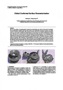
Figure 2. Flowchart depicting the overall process used in this work. Starting with a binary image containing an anatomical structure, we first skeletonize the object. If the skeleton contains N figures, the skeleton points are clustered into N groups; one group per figure. Points on the surface of the binary object are classified, based on the position of the skeleton, as belonging to either the upper or the lower surface of the object. Next, the surfaces represented by the skeleton, upper, and lower surface points are all parameterized via nonlinear dimensionality reduction (see figure 3). This yields, for each figure, meshes for the skeleton, the upper surface, and the lower surface. Correspondence between nodes in these meshes is established in the 2D coordinate systems established during nonlinear dimensionality reduction, and this correspondence is used to compute the thickness vectors.
The overall process followed in this paper is described in figure 2. Given a binary image of an anatomical structure, its skeleton is computed and pruned by an applicable method.6 Skeleton points are then clustered such that each cluster contains a single medial sheet. To do this, we eliminate all voxels having more than 8 26-connected neighbours, and find the resulting connected components, treating each component as a separate sheet. This is justified because it is generally agreed upon that a skeletonization algorithm should yield a singlepixel-wide connected skeleton.6 During the clustering process, we obtain for free the loci of junction points of the sheets: the loci of the removed voxels. These can be used, for example, to locate overloaded nodes at a connection curve in medial patches,5 or hinge atoms in multi-figural m-reps.19 Thus we have a set of clusters of
Proc. of SPIE Vol. 6512 65120X-3
(2D)
(3D) Nonlinear dimensionality reduction
Points
Get surface points
(2D) Sample points on a regular lattice
Points
Point samples
Map samples to 3D mesh vertices (3D)
Surface Mesh
(3D) Binary image
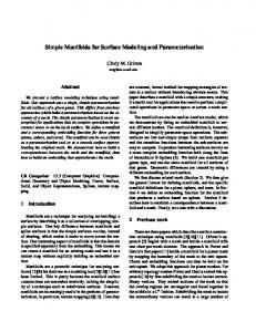
Figure 3. The process used to parameterize a 2D surface embedded in 3D, given a set of disconnected 3D points sampled from the surface. Given a binary image depicting a surface, 3D points are extracted that lie on that surface. Next, these points serve as input to an algorithm for nonlinear dimensionality reduction (ISOMAP11 is used in this work) in order to map the points into their intrinsic 2D space. Points are then sampled from this 2D space based on a regular lattice, and these point samples are mapped back to 3D using information derived from the mapping discovered by ISOMAP. The mapped 3D points form the vertices of a surface mesh, and the edges of the mesh connect neighbours according to the 2D lattice.
medial voxels, where the voxels in each cluster are taken to be samples from a single (likely non-planar) surface in 3D, corresponding to a single-figural part of the anatomical structure. Next, we assign a label to each object surface voxel as belonging to the upper or lower surface of the object, depending on which side of the object’s skeleton the point lies. Thus, for each figure, we have three sets of 3D points: medial surface, upper surface, and lower surface. Next, we learn the parameters of the intrinsic 2D coordinate systems of the surfaces from which each of these point sets were sampled via nonlinear dimensionality reduction. This process is depicted in figure 3 and is discussed below; for the moment we will treat this as a black box. The output of surface parameterization is, for each figure, three meshes, each with N × M vertices, depicting the medial surface, the upper surface, and the lower surface. Remembering that each 3D mesh vertex corresponds to a set of 2D (i, j) parameters obtained during manifold learning, we form thickness vectors emanating from each vertex (i, j) on the medial surface to corresponding vertices (i, j) on the upper and lower surfaces. We have thus computed the basic building blocks for a medial representation of the figure: a medial sheet consisting of a set of connected nodes, and a set of thickness vectors emanating from each of the nodes to the surface. j
z
j
z
y
y x
(a)
i
(b)
x
i
(c)
(d)
Figure 4. Pictorial illustration of surface parameterization. (a) Collection of 3D points (red) sampled from a surface. (b) Points mapped to 2D via mapping M obtained from manifold learning. (c) Regular mesh created within the surface in a 2D (i, j) coordinate system. (d) Mesh and (i, j) parameterization mapped back to 3D using inverse of M .
We now turn our attention to the surface parameterization process depicted in figure 3. Given a 3D binary image depicting a surface of interest, we extract the 3D points lying on the surface. Next, we perform nonlinear dimensionality reduction, also known as manifold learning, using the ISOMAP method.11 ISOMAP forms a neighbourhood graph with the 3D points as nodes, with edges between each node and its nearest neighbours in 3D. The edges are weighted according to the euclidean distance between neighbouring nodes. The geodesic
Proc. of SPIE Vol. 6512 65120X-4
distance between each pair of points is computed by integrating the graph edge weights along the shortest path between the points. A distance matrix is thus formed and used in classical multi-dimensional scaling in order to perform dimensionality reduction preserving inter-point geodesic distances, both locally and globally. Here, we use ISOMAP to reduce the dimensionality of the 3D points P to 2D points Q, illustrated in figure 4. Because ISOMAP is a geodesic distance-preserving mapping, the resulting 2D coordinates are intrinsic to the 2-manifold sampled by the skeleton points. Next, we center an N × M regular lattice of 2D nodes on the region containing points Q. This is done by setting a margin size for the region, and overlaying the regular lattice to fill the entire region specified by the margin size. The motivation for the use of a margin is that in practice, we do not want medial or surface nodes to fully extend to the edges of the skeleton or upper and lower surfaces. These nodes form vertices of a quad mesh where edges join 4-connected neighbours. Lastly, each vertex V of the mesh is mapped back to 3D by trilinear interpolation of points P corresponding to neighbours N ∈ Q of V . The end result of this process is that mesh vertices have equal geodesic spacing along the surface.
4. RESULTS
(a)
(b)
J (c)
(d)
Figure 5. (a) Left thalamus binary image (blue) with skeleton points (green) shown within. (b) Mesh resulting from medial sheet parameterization of (a). (c),(d) Similar to (a) and (b), for left caudate nucleus image.
Figure 5 illustrates the parameterization of the medial surfaces of images of the thalamus and caudate nucleus segmented from an MRI of the brain. Specifically, this figure shows the result of applying the process given in figure 3 to a binary image containing a single medial sheet. Parts (a) and (c) show the skeleton points in green,
Proc. of SPIE Vol. 6512 65120X-5
and parts (b) and (d) show the meshes resulting from medial sheet parameterization on a 6 × 8 grid. Manifold learning was conducted with k-ISOMAP,11 k = 8.
(a)
(b)
(c)
(d)
Figure 6. (a) A left caudate nucleus segmented from an MRI of the brain, rendered semitransparently as an isosurface. The medial sheet is rendered as a surface within, with thickness vectors emanating to the parameterized object surface. (b) Similar to (a), for a supraspinatus muscle (part of the rotator cuff in the shoulder) extracted from MRI. (c) The parameterized surfaces of the caudate nucleus shown. The top surface is made translucent and the parameterized skeleton is removed for clarity. (d) Similar to (c), for the supraspinatus.
Figure 6 illustrates the results of applying the entire process given in figure 2 to images containing a caudate nucleus and a supraspinatus muscle (a muscle that forms part of the rotator cuff in the shoulder). In both cases, k-ISOMAP11 was used, with k = 12. Note the even, regular distribution of medial and surface nodes that is a consequence of spacing them along equal geodesic distances along each surface. It is due to this equal geodesic spacing, in combination with the correspondence established in the 2D coordinate systems intrinsic to each surface, that the thickness vectors emanating from the medial surface always contact the correct object surface and do not cross. Figure 7 is an artificial example illustrating the parameterization of an object’s skeleton in the multi-figural case. Figure 7(b) shows results obtained for an artificial multi-sheet skeleton (a), using �-ISOMAP,11 � = 4.
Proc. of SPIE Vol. 6512 65120X-6
(a)
(b)
Figure 7. (a) A multi-sheet skeleton of an artificial object. (b) The result of medial sheet parameterization after clustering. Different medial sheets are indicated with different colours.
5. CONCLUSIONS In this work, we gave a preliminary demonstration of the utility of manifold learning for the computation of the fundamental components of a medial shape representation. The results of our work illustrate that the intrinsic 2D coordinate systems learned by nonlinear dimensionality reduction are useful both in distributing medial and surface nodes with equal geodesic spacing, and also for establishing correspondence, in the 2D domain, between medial nodes and corresponding surface nodes. This correspondence is very useful in specifying the start and end point of thickness vectors emanating from the medial sheet to the object surface. Because of the equal geodesic spacing of the nodes, this approach overcomes problems of missed target and crossing normals that arise when computing thickness vectors to be normal either to the medial sheet or to the object surface, as is typical practice. Furthermore, this approach is noniterative and simple to implement. Future work includes research into automatic selection of manifold learning parameters, such as the number of nodes to use for each medial sheet, the choice of k-ISOMAP versus �-ISOMAP, and the specific setting of k or � for a given figure. It would also be worthwhile to assess the utility of this approach in studies of vasculature and the gastrointestinal tract, where situations involving the coincidence of high bending and thickness are likely to occur.
Acknowledgements The medical data presented in this paper was provided by Dr. Martin McKeown of the Department of Medicine at the University of British Columbia, Vancouver, and by Dr. Mark E. Schweitzer of New York University Medical Center, Hospital for Joint Diseases, New York.
REFERENCES 1. Blum, H.: A Transformation for Extracting New Descriptors of Shape. In Wathen-Dunn, W., ed.: Models for the Perception of Speech and Visual Form, Cambridge, MIT Press (1967) 362–380 2. Hamarneh, G., Abugharbieh, R., McInerney, T.: Medial profiles for modeling deformation and statistical analysis of shape and their use in medical image segmentation. IJSM 10(2) (2004) 187–209 3. Pizer, S., Fletcher, P.T., Joshi, S., Thall, A.: Deformable M-Reps for 3D medical image segmentation. IJCV 55(2-3) (2003) 85–106
Proc. of SPIE Vol. 6512 65120X-7
4. Ward, A.D., Schweitzer, M.E., Hamarneh, G.: Computational and visualization techniques for understanding the shape variations of the bicipital groove of the proximal humerus. Annual meeting of the Society for Computer Applications in Radiology (2006) 47–49 5. Hamarneh, G., Ward, A.D., Frank, R.: Quantification and visualization of localized and intuitive shape variability using a novel medial-based shape representation. Proceedings of IEEE International Symposium on Biomedical Imaging (to appear) (2007) 6. Lee, S.W., Lam, L., Suen, C.Y.: A systematic evaluation of skeletonization algorithms. International J. Pattern Recognition and Artificial Intelligence 7(5) (1993) 1203–1225 7. Palagyi, K.: A 3D 3-subiteration thinning algorithm for medial surfaces. In: DGCI ’00: Proceedings of the 9th International Conference on Discrete Geometry for Computer Imagery, London, UK, Springer-Verlag (2000) 406–417 8. Xu, W., Wang, C.: CGT: A fast thinning algorithm implemented on a sequential computer. IEEE Trans. Syst. Man. Cybern. 17(5) (1987) 847–851 9. Arcelli, C., Cordella, L.P., Levialdi, S.: Parallel thinning of binary pictures. Electronic Letters 11(7) (1975) 148–149 10. Golland, P., Grimson, W.E.L.: Fixed topology skeletons. IEEE Conference on Computer Vision and Pattern Recognition 1 (2000) 10–17 11. Tenenbaum, J.B., De Silva, V., Langford, J.C.: A global geometric framework for nonlinear dimensionality reduction. Science 290 (2000) 3219–2323 12. Roweis, S.T., Saul, L.K.: Nonlinear dimensionality reduction by locally linear embedding. Science 290 (2000) 2323–2326 13. Belkin, M., Niyogi, P.: Laplacian eigenmaps for dimensionality reduction and data representation. Neural Computation 15 (2003) 1373–1396 14. Zigelman, G., Kimmel, R., Kiryati, N.: Texture mapping using surface flattening via multidimensional scaling. IEEE Transactions on Visualization and Computer Graphics 8(2) (2002) 198–207 15. Grossmann, R., Kiryati, N., Kimmel, R.: Computational surface flattening: A voxel-based approach. IEEE Transactions on Pattern Analysis and Machine Intelligence 24(4) (2002) 433–441 16. Liu, Y.S., Yong, J.H., Yu, P.Q., Zhang, H., Du, M.C., Paul, J.C.: Mesh parameterization for an open connected surface without partition. Proceedings of the International Conference on Computer Aided Design and Computer Graphics (2005) 5p 17. Oda, M., Hayashi, Y., Kitasaka, T., Mori, K., Suenaga, Y.: A method for generating virtual unfolded view of colon using spring model. Proceedings of SPIE Medical Imaging 2006: Physiology, Function, and Structure from Medical Images 6143 (2006) 458–469 18. Wang, G., McFarland, G., Brown, B.P., Vannier, M.W.: GI tract unraveling with curved cross sections. IEEE Transactions on Medical Imaging 17(2) (1998) 318–322 19. Han, Q., Lu, C., Lui, G., Pizer, S.M., Joshi, S., Thall, A.: Representing multi-figure anatomical objects. ISBI (2004) 1251–1254
Proc. of SPIE Vol. 6512 65120X-8