A Hybrid Least Square Support Vector Machine Model with ...

Hindawi Publishing Corporation Mathematical Problems in Engineering Volume 2015, Article ID 231394, 7 pages http://dx.doi.org/10.1155/2015/231394

Research Article A Hybrid Least Square Support Vector Machine Model with Parameters Optimization for Stock Forecasting Jian Chai,1 Jiangze Du,2 Kin Keung Lai,1,2 and Yan Pui Lee3 1

International Business School, Shaanxi Normal University, Xian 710062, China Department of Management Sciences, City University of Hong Kong, Hong Kong 3 School of Business, Tung Wah College, Hong Kong 2

Correspondence should be addressed to Kin Keung Lai; [email protected] Received 30 May 2014; Accepted 20 August 2014 Academic Editor: Shifei Ding Copyright © 2015 Jian Chai et al. This is an open access article distributed under the Creative Commons Attribution License, which permits unrestricted use, distribution, and reproduction in any medium, provided the original work is properly cited. This paper proposes an EMD-LSSVM (empirical mode decomposition least squares support vector machine) model to analyze the CSI 300 index. A WD-LSSVM (wavelet denoising least squares support machine) is also proposed as a benchmark to compare with the performance of EMD-LSSVM. Since parameters selection is vital to the performance of the model, different optimization methods are used, including simplex, GS (grid search), PSO (particle swarm optimization), and GA (genetic algorithm). Experimental results show that the EMD-LSSVM model with GS algorithm outperforms other methods in predicting stock market movement direction.

1. Introduction Stock market is one of the most sophisticated and challenging financial markets since many factors affect its movement, including government policy, global economic situation, investors’ expectations, and even correlations with other markets [1]. References [2, 3] described financial time series as essentially noisy, dynamic, and deterministically chaotic data sequences. Hence, a precise prediction of stock index movement can help investors make decisions to take or shed positions in the stock market at the right time and make profits. Many works have been published by researchers to maximize investment profits and minimize risk. Therefore, predicting stock market is quite important and significant. Neural networks have been successfully applied in forecasting of financial time series during the past two decades [4–6]. Neural networks are general function approximations which can approximate many nonlinear functions regardless of the properties of time series data [7]. Besides, neural networks are able to learn dynamic systems which make them a more powerful tool for studying financial time series compared with traditional models [8–10]. However, there are a couple of weaknesses when neural networks are used

in forecasting financial time series. For instance, when the typical back-propagation neural network is applied, a huge number of parameters are required to be controlled for. This makes the solution unstable and causes overfitting. The overfitting problem results in poor performance and becomes a critical issue for researchers. Accordingly, [11] proposed a support vector machine (SVM) model. According to [12–14], there are two advantages of using SVM rather than neural networks. One is that SVM has a better performance in terms of generalization. Unlike the empirical risk minimization principle in traditional neural networks, SVM reduces generalization error bounds based on the structural risk minimization principle. SVM seeks to achieve an optimal structure through finding out a balance between generalization errors and VapnikChervonenkis (VC) confidence interval. Another advantage is that SVM prevents the model from getting stuck into local minima. Since the introduction of SVM, it has been developed rapidly in the real world. There are mainly two ways for applying SVM: one is classification and the other is regression. For classification, [15] constructed a SVM based model to accurately evaluate the consumers’ credit score and solve

2

Mathematical Problems in Engineering

classification problems. Also, SVM is widely used in the area of forecasting. Reference [16] used SVM to predict the direction of daily stock price in the Korea composite stock price index (KOSPI). More recently, [17] applies the Support Vector Regression to forecast the Nikki 225 opening index and TAIEX closing index after detecting and removing the noise by independent component analysis (ICA). However, the performance of SVM mainly depends on the input data and is sensitive to parameters. Recent empirical studies have demonstrated that properties of the model performance are influenced by two aspects: low level of signal to noise ratio (SNR) and instability of model specification during the estimation process. For example, [18] investigates the hyperparameters selection for support vector machine with different noise distributions to compare the model performance. Moreover, [19] applied wavelet to denoise the bearing vibration signals by improving the SNR and then figure out the best model according to the performances of ANN and SVM. To improve the classification and forecasting accuracy, several researchers including [20, 21] have proved that the combined classifying and forecasting models perform better than any individual model. Also, [22] showed that the ensemble empirical model decomposition (EEMD) can be integrated with extreme learning machine (ELM) to an effective forecasting model for computer products sales. In this paper, we propose a hybrid EMD-LSSVM (empirical mode decomposition least squares support vector machine) with different parameters optimization algorithms. The experimental results prove that the EMD-LSSVM model has a better performance than the WD-LSSVM (wavelet denoising least squares support vector machine) model. Firstly, we use the empirical mode decomposition and wavelet denoising algorithm to deal with the original input data. Secondly, parameters of SVM are optimized by different methods, including simplex, grid search (GS), particle swarm optimization (PSO), and genetic algorithm (GA). Results from empirical studies show that the hybrid model EMDLSSVM with GS parameter optimization outperforms the other model.

2. EMD-LSSVM Model and WD-LSSVM 2.1. Empirical Mode Decomposition (EMD). References [23, 24] proposed empirical mode decomposition (EMD) which decomposes data series into a number of intrinsic mode functions (IMFs). It was designed for nonstationary and nonlinear data sets. In order to apply EMD, time series data set must satisfy the following two conditions. (1) The sum of local maxima and local minima must equate to the total number of zero crossings or the difference between them is 1. In other words, for every local maxima and local minima, there must be one zero crossing following up. (2) The local average is zero, which means that mean value of the upper envelope (defined by local maxima) and lower envelope (defined by local minima) must be zero.

Thus, if a function is an IMF, it represents a signal symmetric to local mean zero. An IMF is a simple oscillatory mode which is more general than the simple harmonic function and the frequency and amplitude of the IMF can be variable. Then, data series 𝑥(𝑡) (𝑡 = 1, 2, . . . , 𝑛) can be decomposed by the following sifting procedure. (1) Find all local maxima and minima in 𝑥(𝑡). Then use the cubic spline line to connect all local maxima to generate upper envelope 𝑥up (𝑡) and connect all local minima to generate lower envelop 𝑥low (𝑡). (2) According to the upper and lower envelopes obtained in Step (1), calculate the envelope mean 𝑚1 (𝑡): 𝑚1 (𝑡) =

(𝑥up (𝑡) + 𝑥low (𝑡)) 2

.

(1)

(3) Data series 𝑥(𝑡) minus envelope mean 𝑚1 (𝑡) gives the first component 𝑑1 (𝑡): 𝑑1 (𝑡) = 𝑥 (𝑡) − 𝑚1 (𝑡) .

(2)

(4) Check if 𝑑1 (𝑡) satisfies the IMF requirements; if 𝑑1 (𝑡) does not satisfy them, go back to Step (1) and replace 𝑥(𝑡) with 𝑑1 (𝑡) to conduct the second sifting procedure; that is, 𝑑2 (𝑡) = 𝑑1 (𝑡) − 𝑚2 (𝑡). Repeat the sifting procedure 𝑘 times 𝑑𝑘 (𝑡) = 𝑑𝑘−1 (𝑡) − 𝑚𝑘 (𝑡) until the following stop criterion is satisfied: 𝑇

[𝑑𝑗 (𝑡) − 𝑑𝑗+1 (𝑡)]

𝑡=1

𝑑𝑗2 (𝑡)

∑

2

< SC,

(3)

where SC is the stopping condition. Normally, it is set between 0.2 and 0.3. Then, we get the first IMF component; that is, 𝑐1 (𝑡) = 𝑑𝑘 (𝑡). (5) Subtract first IMF component 𝑐1 (𝑡) from data sets 𝑥(𝑡) and get the residual 𝑟1 (𝑡) = 𝑥(𝑡) − 𝑐1 (𝑡). (6) Treat 𝑟1 (𝑡) as the new data series and repeat Steps (1) to (5). Then get the new residual 𝑟2 (𝑡). In this way, after repeating 𝑛 times, we get 𝑟2 (𝑡) = 𝑟1 (𝑡) − 𝑐2 (𝑡) , 𝑟3 (𝑡) = 𝑟2 (𝑡) − 𝑐3 (𝑡) , (4)

.. . 𝑟𝑛 (𝑡) = 𝑟𝑛−1 (𝑡) − 𝑐𝑛 (𝑡) .

When the residual 𝑟𝑛 (𝑡) becomes a monotonic function, the data sets cannot be decomposed anymore. The whole EMD is completed. The original date series can be described as the combination of 𝑛 IMF components and a mean trend 𝑟𝑛 (𝑡); that is, 𝑛

𝑥 (𝑡) = ∑ 𝑐𝑗 (𝑡) + 𝑟𝑛 (𝑡) . 𝑗=1

(5)

Mathematical Problems in Engineering

3

In this way, the original data series 𝑥(𝑡) can be decomposed into 𝑛 IMFs and a mean trend function. Then, we use the IMFs for instantaneous frequency analysis. The traditional Fourier transform decomposes a data series into a number of sine or cosine waves for the analysis. However, the EMD technique decomposes the data series into several sinusoid-like signals with variable frequencies and a mean trend function. The EMD has several advantages. First, this method is relatively easy to understand and is also widely applied since it avoids complex mathematical algorithms. Secondly, EMD is suitable to deal with nonlinear and nonstationary data series. Thirdly, EMD is more suitable for analysing data series with trends such as weather and economic data. Finally, EMD is able to find the residual which reveals the data series trends [25–27]. 2.2. Wavelet Denoising Algorithm. While the traditional Fourier analysis can only remove noise of certain patterns over the entire time horizon, wavelet analysis can deal with multiscales and more detailed data and is more suitable for financial time series. Wavelets are continuous functions which satisfy the unit energy and admissibility condition in 𝐶𝜑 = ∫

∞

0

󵄨 󵄨󵄨 󵄨󵄨𝜑 (𝑓)󵄨󵄨󵄨 𝑑𝑓 < ∞, 𝑓

∞

󵄨2 󵄨󵄨 󵄨󵄨𝜓 (𝑡)󵄨󵄨󵄨 𝑑𝑡 = 1, −∞

∫

(6)

we apply 𝜑(𝑥) to map 𝑥𝑘 from 𝑅𝑛 to 𝑅𝑛ℎ . Notice that 𝜑(𝑥) can be of infinite dimensional and is defined only implicitly. Also, vector 𝜔 can also be infinite dimensional. Thus, the optimization problem becomes min s.t.

∞

−∞

𝑥 (𝑡)

1 𝑡−𝑢 𝜓( ) 𝑑𝑡, √𝑠 𝑠

𝑘 = 1, . . . , 𝑁,

𝜔𝑇 𝜑 (𝑥𝑘 ) + 𝑏 − 𝑦𝑘 ≤ 𝜀 + 𝜉𝑘∗ ,

𝑘 = 1, . . . , 𝑁,

(9)

𝑘 = 1, . . . , 𝑁.

The constant 𝑐 > 0 defines the tolerance of deviations from the desired 𝜀 accuracy. It defines the weight of the regularization term empirical risk. The larger the c is, the more important it is for the empirical risk to grow, compared with the regularization term. 𝜀 is called the tube size and represents the accuracy required in training data points. By introducing Lagrange multipliers 𝛼, 𝛼∗ , 𝜂, 𝜂∗ ≥ 0, we obtain the Lagrangian for this problem. Consider 𝐿 (𝜔, 𝑏, 𝜉𝑘 , 𝜉𝑘∗ ; 𝛼, 𝛼∗ , 𝜂, 𝜂∗ ) 𝑁 1 = 𝜔𝑇 𝜔 + 𝑐 ∑ (𝜉 + 𝜉∗ ) 2 𝑘=1 𝑁

− ∑ 𝛼𝑘 (𝜀 + 𝜉𝑘 − 𝑦𝑘 + 𝜔𝑇 𝜑 (𝑥𝑘 ) + 𝑏) 𝑘=1

(10)

𝑁

− ∑ 𝛼𝑘∗ (𝜀 + 𝜉𝑘∗ + 𝑦𝑘 − 𝜔𝑇 𝜑 (𝑥𝑘 ) − 𝑏)

(7)

𝑘=1

where u is the dilation parameter and s is the translation parameter. The wavelet synthesis rebuilds the original data series, guaranteed by the properties of orthogonal transformation in 𝑑𝑠 1 ∞ ∞ 𝑥 (𝑡) = ∫ ∫ 𝑊 (𝑢, 𝑠) 𝜓𝑢,𝑠 (𝑡) 𝑑𝑢 2 . 𝐶𝜓 0 −∞ 𝑠

𝑦𝑘 − 𝜔𝑇 𝜑 (𝑥𝑘 ) − 𝑏 ≤ 𝜀 + 𝜉𝑘 ,

𝜉𝑘 , 𝜉𝑘∗ ≥ 0,

where 𝜑 is the Fourier transform of frequency𝑓. 𝜓 is the wavelet transform. The continuous wavelet function can orthogonally transform the original data into subdata series in the wavelet domain. Consider 𝑊 (𝑢, 𝑠) = ∫

𝑁 1 𝐽𝑃 (𝜔, 𝜉, 𝜉∗ ) = 𝜔𝑇 𝜔 + 𝑐 ∑ (𝜉 + 𝜉∗ ) , 2 𝑘=1

(8)

In wavelet analysis, the denoising technique separates the data and noise from the original data sets by selecting a threshold. The raw data series are first decomposed into some data subsets. Then, based on a certain strategy of selecting the threshold, the boundary between noises and data is set. Depending on the boundary, smaller data points are eliminated and the remaining data are handled by setting certain thresholds. Finally, these denoised data sets are rebuilt from the decomposed data points [28]. 2.3. LSSVM in Function Estimation. This section shows the basic theory of the least squares support vector machine. The support vector methodology has been used mainly in two areas, that is, classification and function estimation. Considering regression in the set of function 𝑓(𝑥) = 𝜔𝑇 𝜑(𝑥) + 𝑏 with given training data inputs 𝑥𝑘 ∈ 𝑅𝑛 and outputs 𝑦𝑘 ∈ 𝑅,

𝑁

− ∑ (𝜂𝑘 𝜉𝑘 + 𝜂𝑘∗ 𝜉𝑘∗ ) . 𝑘=1

The reason of introducing another Lagrange multiplier 𝛼𝑘∗ is that there are other slack variables 𝜉𝑘 , 𝜉𝑘∗ . By maximizing the Lagrangian max min 𝐿 (𝜔, 𝑏, 𝜉𝑘 , 𝜉𝑘∗ ; 𝛼, 𝛼∗ , 𝜂, 𝜂∗ ) ,

𝛼,𝛼∗ ,𝜂,𝜂∗ 𝜔,𝑏,𝜉𝑘 ,𝜉𝑘∗

(11)

we obtain 𝑁 𝜕𝐿 = 0 󳨀→ 𝜔 = ∑ (𝛼𝑘 − 𝛼𝑘∗ ) 𝜑 (𝑥𝑘 ) , 𝜕𝜔 𝑘=1 𝑁 𝜕𝐿 = 0 󳨀→ ∑ (𝛼𝑘 − 𝛼𝑘∗ ) = 0, 𝜕𝑏 𝑘=1

𝜕𝐿 = 0 󳨀→ 𝑐 − 𝛼𝑘 − 𝜂𝑘 = 0, 𝜕𝜉𝑘 𝜕𝐿 = 0 󳨀→ 𝑐 − 𝛼𝑘∗ − 𝜂𝑘∗ = 0. 𝜕𝜉𝑘∗

(12)

4

Mathematical Problems in Engineering Table 1: Input and output variables.

Category Training and validation testing

Input variables selection

Output variable

Sample

Data number

CSI 300, USDX, SHIBOR, REPO, CDS, PE, M2/mkt cap, short-mid not/mkt cap, New Loan/mkt cap

CSI 300

05/01/2009–23/08/2011 24/08/2011–20/01/2012

643 100

Then we obtain the following dual problem: max ∗ 𝛼,𝛼

1 𝑁 𝐽𝐷 (𝛼, 𝛼∗ ) = − ∑ (𝛼𝑘 − 𝛼𝑘∗ ) (𝛼𝑙 − 𝛼𝑙∗ ) 𝐾 (𝑥𝑘 , 𝑥𝑙 ) 2𝑘=1 𝑁

𝑁

𝑘=1

𝑘=1

− 𝜀 ∑ (𝛼𝑘 + 𝛼𝑘∗ ) + ∑ 𝑦𝑘 (𝛼𝑘 − 𝛼𝑘∗ ) , 𝑁

s.t.

∑ (𝛼𝑘 − 𝛼𝑘∗ ) = 0,

𝑘=1

𝛼𝑘 , 𝛼𝑘∗ ∈ [0, 𝑐] . (13)

Here we use the kernel function 𝐾(𝑥𝑘 , 𝑥𝑙 ) = 𝜑(𝑥𝑘 )𝑇 𝜑(𝑥𝑙 ) for 𝑘, 𝑙 = 1, . . . , 𝑁. Then the function estimation becomes 𝑁

𝑓 (𝑥) = ∑ (𝛼𝑘 − 𝛼𝑘∗ ) 𝐾 (𝑥𝑘 , 𝑥𝑙 ) + 𝑏,

(14)

𝑘=1

where 𝛼𝑘 , 𝛼𝑘∗ are solutions of the above quadratic programming problem and 𝑏 is obtained from the complementarity of KKT conditions. It is obvious that the decision function is determined by the support vectors in which coefficients (𝛼𝑘 − 𝛼𝑘∗ ) are not zero. In practice, a larger 𝜀 results in a smaller number of support vectors and thus the sparser of the solution. Also, the larger the 𝜀 is, the worse the accuracy of training points will be. Hence, 𝜀 can be applied to control the balance between closeness to training data and sparseness of the solution. Kernel function can be obtained by seeking the function which satisfies Mercer’s condition. Here are some popular kernel functions [14, 29, 30]: linear: 𝐾(𝑥, 𝑥𝑘 ) = 𝑥𝑇𝑥𝑘 ; polynomial: 𝐾(𝑥, 𝑥𝑘 ) = (𝑥𝑇 𝑥𝑙 + 1)𝑑 , where 𝑑 is the degree of the polynomial kernel; RBF kernel: 𝐾(𝑥, 𝑥𝑘 ) = exp(−‖𝑥 − 𝑥𝑘 ‖2 /𝜎2 ), where 𝜎2 is the bandwidth of the Gaussian kernel. Parameters of the kernel function define the structure of the high dimensional feature space 𝜑(𝑥) and also control the accuracy of the final solution. Thus, they should be selected carefully.

3. Empirical Study 3.1. Data Description. The CSI 300 is chosen for empirical analysis and to examine the performance of the proposed model. This index comprises 179 stocks from Shanghai stock

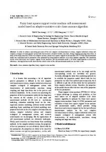
exchange and 121 stocks from Shenzhen stock exchange and is managed by the China Securities Index Company Ltd. Most researchers have chosen international indices in the past, including S & P 500, NIKKEI 225, NASDAQ, DAX, and gold price as input variables. They have examined the cross relationship between stock market index and macroeconomic variables. The potential input variables that can be used for forecasting model mainly consist of the gross domestic product (GDP), gross national product (GNP), short-term interest rate (ST), long-term interest rate (LT), and term structure of interest rate (TS) [1, 31, 32]. Although China has overtaken Japan to become the world’s second largest economy and the Chinese stock market has developed into one of the most important markets in the global economy, Chinese consumption capacity is limited in the domestic market. The movement of the stock market has a close relationship with the money available of the investors, which is determined by the money supply and the interest rate. Considering that the Chinese stock market is affected by the global economic situation as well as the domestic economic development, we choose US Dollar Index (USDX), Shanghai Interbank Offered Rate (SHIBOR), P/E ratio (PE), money supply (M2), repurchase agreement (REPO), China CNY Monthly New Loan, market capitalization of the 300 publicly traded companies (mkt cap), People’s Bank 5-year CDS, and short-mid note as input variables. The lag of input variables is 3 days. We use the daily data to predict the CSI 300 index by nonlinear SVM regression. Since M2, short-mid note, and New Loan are published once a month, we transform these variables into daily variables by dividing them by a daily variable. We divided all data sets into two sections and used the first section as the training part to find the optimal parameters for the LSSVM and avoid overfitting by training and validating the model. The other section is used for testing. As shown in Table 1, we choose nine variables as the input variables and one variable as the output variable including 643 daily data from May 1, 2009, to August 23, 2011, to train the parameters in the model. Once we obtain these parameters, we use the same input and output variables from August 24, 2011, to January 20, 2012, including 100 daily data to examine the performance of different model in the testing part. In the hybrid wavelet denoising least squares support vector machine model (WD-LSSVM), we first denoise the CSI 300 index with wavelet denoising technique. As shown in Figure 1, the original data, which is depicted in the upper part of the figure, is packed with irrelevant noise. Then the wavelet denoising algorithm is applied to reduce the noise in the upper figure of Figure 1. The denoised data is depicted in the lower part of Figure 1 and it is clear that the denoised data

CSI 300 index

CSI 300 index

Mathematical Problems in Engineering

4000 3500 3000 2500 2000 1500

4000 3500 3000 2500 2000 1500

Metrics NMSE 05/05/2009 28/12/2009 10/07/2010 21/01/2011 23/08/2010 Date (dd/mm/yy)

MAPE

Calculation 2 𝑛 ∑ (𝑎 − 𝑝𝑖 ) NMSE = 𝑖=1 2𝑖 𝛿𝑛 2 𝑛 ∑𝑖=1 (𝑎𝑖 − 𝑎) 2 𝛿 = 𝑛−1 1 𝑛 󵄨󵄨󵄨 𝑎 − 𝑝𝑖 󵄨󵄨󵄨󵄨 MAPE = ∑ 󵄨󵄨󵄨 𝑖 󵄨 × 100% 𝑛 𝑖=1 󵄨󵄨 𝑝𝑖 󵄨󵄨󵄨 𝑛

Denoised data

HR =

HR

05/05/2009 28/12/2009 10/07/2010 21/01/2011 23/08/2010 Date (dd/mm/yy)

Table 2: Parameters setting for simplex, GS, GA, and PSO. Method

Parameter setting

Simplex GS

Chi: 2, Gamma: 0.5, Rho: 1, Sigma: 0.5 TolX: 0.001, maxFunEvals: 70, grain: 7, zoomfactor: 5 Sizepop: 20, maxgen: 200, 𝑐min: 0, 𝑐max: 100, 𝑔min: 0, 𝑔max: 1000 Sizepop: 20, maxgen: 200, 𝑐min: 0, 𝑐max: 100, 𝑔min: 0, 𝑔max: 1000, 𝑘: 0.6

PSO

Table 3: Performance metrics and their calculations.

Original data

Figure 1: The original and denoised daily CSI 300 index.

GA

5

can better reveal the trend of the index. Also, in both EMDLSSVM and WD-LSSVM models, we preprocess the input data by scaling to the range of [0, 1] to prevent small numbers in the data sets from being overshadowed by large numbers, resulting in loss of information. 3.2. Optimization Methods and Parameters Setting. In both EMD-LSSVM models and WD-LSSVM, we try four kinds of search methods, that is, simplex, GS, GA, and PSO. In the simplex method, we define the parameters of expanding (Chi), contracting (Gamma), reflecting (Rho), and shrinking (Sigma) and get the optimal parameters for SVM through iteration until the stopping criteria is satisfied. Also, by calculating the objective function, we can get all points in the grids, which are related to the range and the unit grid search size. The optimal parameters can be obtained from the point which has the lowest cost. Another effective method to solve optimization problem is the genetic algorithm. The first step of this method is to randomly select parents from the population. Then, parents produce children continuously. Step by step, the population eventually develops and optimal solution can be obtained when the stopping criteria are met. The PSO algorithm works by moving the candidate solution (particles) within the given search range. These particles are moved by the best known positions of particles and the entire

∑𝑖=1 𝑑𝑖

𝑛 {1 if (𝑎𝑖 − 𝑎𝑖−1 ) (𝑝𝑖 − 𝑝𝑖−1 ) ≥ 0 𝑑𝑖 = { {0 otherwise Table 4: Results of eight different forecasting models.

Model EMD-LSSVM (simplex) EMD-LSSVM (GS) EMD-LSSVM (GA) EMD-LSSVM (PSO) WD-LSSVM (simplex) WD-LSSVM (GS) WD-LSSVM (GA) WD-LSSVM (PSO)

NMSE 0.0253 0.0245 2.5749 9.4471 0.0521 0.0609 0.0657 0.0910

MAPE 0.79222% 0.78834% 9.0641% 18.2733% 1.1772% 1.1357% 1.2997% 1.5072%

HR 77.7778% 79.798% 42.4242% 40.404% 65.6566% 61.6162% 62.6263% 63.6364%

swarm in the search space. When the particles arrive at a better position, they guide the swarm to move. The procedure is repeated until the stopping criteria are satisfied. In our experiment, Table 2 shows the setting of each optimization method. 3.3. Performance Criteria. We evaluate the performance of these models using three measurement methods, that is, normalized mean squared error (NMSE), mean absolute percentage error (MAPE), and the hitting ratio (HR) (Table 3). NMSE and MAPE are designed to measure the deviation of predicted value from the actual value; smaller values of NMSE and MAPE indicate better performance of the model. In the stock market, smaller values of MAPE and NMSE are able to control investment risk. We also introduce hitting rate to evaluate the model since the HR reveals accuracy of prediction of the CSI 300, which is valuable for individual and institutional traders. 3.4. Experiment Results. The experiments explore four parameter selection methods in both EMD-LSSVM and WDLSSVM. Results of the experiments are as in Table 4. From the results, we can see that the hybrid model EMD-LSSVM with GS parameter optimization method not only has the smallest NMSE and MAPE but also gets the best hitting rate, which means it outperforms the other model with different parameter search methods. From the experiment results, we can draw three conclusions.

6

Mathematical Problems in Engineering (1) For overall accuracy, the EMD-LSSVM (GS) is the best approach, followed by EMD-LSSVM (simplex), WD-LSSVM (simplex), WD-LSSVM (PSO), WDLSSVM (GA), and WD-LSSVM (GS). Hitting rates of the other approaches are below 60%. Prediction accuracy of all methods is also related to the chosen sample. So it is difficult to identify which model is the best and performs the best. However, tests based on the same sample may help us identify which is the best model. (2) According to the experiments, the PSO and GA need more computational time to obtain the best parameters for the model compared with simplex and GS optimization methods. Although the PSO and GA algorithm are relatively more complex than the other two methods, they do not perform better than GS and simplex. (3) Another interesting finding is that thresholds of the denoising algorithm also influence the performance of the model. When the threshold is too large, useful information in the data gets damaged. Besides, a small threshold makes the denoising process insignificant for handling noise. Therefore, we argue that the performance of the wavelet denoising algorithm is sensitive to the estimation method of the threshold level.

4. Conclusion We have examined the use of the hybrid EMD-LSSVM and WD-LSSVM models to predict financial time series by four different parameters selection methods in this paper. The study shows that the hybrid EMD-LSSVM model provides a better way to forecast financial time series compared with WD-LSSVM. The key findings contain two aspects. First, empirical mode decomposition can serve as a potential tool for removing noise from original data during the modeling process and improving the prediction accuracy. Second, we compare four kinds of search methods for parameters in the experiments. The results show that the EMD-LSSVM with GS parameter optimization method provides the best performance. Use of the GS algorithm reduces the computation time and improves the prediction accuracy of the model for forecasting financial time series. Future research in this direction mainly includes gaining better understanding of the relationship between optimal loss function, noise distribution, and the number of training samples. In this paper, we only consider applying different algorithm to denoise the original data without considering the distribution of the noise. The research on the density of noise which will be reduced for the SVM model will attract the effort of us. Moreover, another interesting research direction is to figure out the minimum number of samples based on which a theoretically optimal loss function will indeed have superior generalization performance.

Conflict of Interests The authors declare that there is no conflict of interests regarding the publication of this paper.

References [1] W. Huang, Y. Nakamori, and S.-Y. Wang, “Forecasting stock market movement direction with support vector machine,” Computers and Operations Research, vol. 32, no. 10, pp. 2513– 2522, 2005. [2] J. W. Hall, “Adaptive selection of U.S. stocks with neural nets,” in Trading on the Edge: Neural, Genetic, and Fuzzy Systems for Chaotic Financial Markets, G. J. Deboeck, Ed., John Wiley & Sons, New York, NY, USA, 1994. [3] Y. S. Abu-Mostafa and A. F. Atiya, “Introduction to financial forecasting,” Applied Intelligence, vol. 6, no. 3, pp. 205–213, 1996. [4] W. Cheng, L. Wagner, and C.-H. Lin, “Forecasting the 30-year US treasury bond with a system of neural networks,” Journal of Computational Intelligence in Finance, vol. 4, pp. 10–16, 1996. [5] R. Sharda and R. B. Patil, “A connectionist approach to time series prediction: an empirical test,” in Neural Networks in Finance and Investing: Using Artificial Intelligence to Improve Real World Performance, R. R. Trippi and E. Turban, Eds., Irwin Professional Publishing, Chicago, Ill, USA, 1996. [6] J. R. van Eyden, The Application of Neural Networks in the Forecasting of Share Prices, Finance and Technology Publishing, Haymarket, Va, USA, 1996. [7] I. Kaastra and M. S. Boyd, “Forecasting futures trading volume using neural networks,” Journal of Futures Markets, vol. 15, pp. 853–970, 1995. [8] G. Zhang and M. Y. Hu, “Neural network forecasting of the British pound/US dollar exchange rate,” Omega, vol. 26, no. 4, pp. 495–506, 1998. [9] W.-C. Chiang, T. L. Urban, and G. W. Baldridge, “A neural network approach to mutual fund net asset value forecasting,” Omega, vol. 24, no. 2, pp. 205–215, 1996. [10] F. E. H. Tay and L. Cao, “Application of support vector machines in financial time series forecasting,” Omega, vol. 29, no. 4, pp. 309–317, 2001. [11] V. N. Vapnik, The Nature of Statistical Learning Theory, Springer, New York, NY, USA, 2nd edition, 2000. [12] K.-R. Muller, A. J. Smola, G. Ratsch, B. Scholkopf, J. Kohlmorgen, and V. N. Vapnik, “Predicting time series with support vector machines,” in Proceedings of the International Conference on Artificial Neural Networks, pp. 999–1004, Lausanne, Switzerland, 1997. [13] S. Mukherjee, E. Osuna, and F. Girosi, “Nonlinear prediction of chaotic time series using support vector machines,” in Proceedings of the IEEE Workshop on Neural Networks for Signal Processing (NNSP ’97), pp. 511–520, Amelia Island, Fla, USA, September 1997. [14] V. N. Vapnik, S. E. Golowich, and A. Smola, “Support vector method for function approximation, regression estimation, and signal processing,” Advances in Neural Information Processing Systems, vol. 9, pp. 281–287, 1996. [15] C.-L. Huang, M.-C. Chen, and C.-J. Wang, “Credit scoring with a data mining approach based on support vector machines,” Expert Systems with Applications, vol. 33, no. 4, pp. 847–856, 2007.

Mathematical Problems in Engineering [16] K.-J. Kim, “Financial time series forecasting using support vector machines,” Neurocomputing, vol. 55, no. 1-2, pp. 307–319, 2003. [17] C.-J. Lu, T.-S. Lee, and C.-C. Chiu, “Financial time series forecasting using independent component analysis and support vector regression,” Decision Support Systems, vol. 47, no. 2, pp. 115–125, 2009. [18] V. Cherkassky and Y. Ma, “Practical selection of SVM parameters and noise estimation for SVM regression,” Neural Networks, vol. 17, no. 1, pp. 113–126, 2004. [19] G. S. Vijay, H. S. Kumar, P. P. Srinivasa, N. S. Sriram, and R. B. K. N. Rao, “Evaluation of effectiveness of wavelet based denoising schemes using ANN and SVM for bearing condition classification,” Computational Intelligence and Neuroscience, vol. 2012, Article ID 582453, 12 pages, 2012. [20] L. Zhou, K. K. Lai, and L. Yu, “Least squares support vector machines ensemble models for credit scoring,” Expert Systems with Applications, vol. 37, no. 1, pp. 127–133, 2010. [21] Y. Bao, X. Zhang, L. Yu, K. K. Lai, and S. Wang, “An integrated model using wavelet decomposition and least squares support vector machines for monthly crude oil prices forecasting,” New Mathematics and Natural Computation, vol. 7, no. 2, pp. 299–311, 2011. [22] C.-J. Lu and Y. E. Shao, “Forecasting computer products sales by integrating ensemble empirical mode decomposition and extreme learning machine,” Mathematical Problems in Engineering, vol. 2012, Article ID 831201, 15 pages, 2012. [23] N. E. Huang, Z. Shen, S. R. Long et al., “The empirical mode decomposition and the Hilbert spectrum for nonlinear and non-stationary time series analysis,” The Royal Society of London. Proceedings A: Mathematical, Physical and Engineering Sciences, vol. 454, no. 1971, pp. 903–995, 1998. [24] N. E. Huang, Z. Shen, and S. R. Long, “A new view of nonlinear water waves: the Hilbert spectrum,” Annual Review of Fluid Mechanics, vol. 31, pp. 417–457, 1999. [25] L. Yu, S. Wang, and K. K. Lai, “An EMD-based neural network ensemble learning model for world crude oil spot price forecasting,” in Soft Computing Applications in Business, B. Prasad, Ed., vol. 230 of Studies in Fuzziness and Soft Computing, pp. 261–271, Springer, 2008. [26] L. Yu, K. K. Lai, S. Wang, and K. He, “Oil price forecasting with an EMD-based multiscale neural network learning paradigm,” in International Conference on Computational Science, pp. 925– 932, 2007. [27] S. Zhou and K. K. Lai, “An improved EMD online learningbased model for gold market forecasting,” in Proceedings of the 3rd International Conference on Intelligent Decision Technologies, pp. 75–84, 2011. [28] K. He, C. Xie, and K. K. Lai, “Estimating real estate valueat-risk using wavelet denoising and time series model,” in Computational Science—ICCS 2008, vol. 5102 of Lecture Notes in Computer Science, pp. 494–503, Springer, Berlin, Germany, 2008. [29] S. Zhou, K. K. Lai, and J. Yen, “A dynamic meta-learning ratebased model for gold market forecasting,” Expert Systems with Applications, vol. 39, no. 6, pp. 6168–6173, 2012. [30] C.-W. Hsu, C.-C. Chang, and C.-J. Lin, A Practical Guide to Support Vector Classification, Department of Computer Science and Information Engineering, University of National Taiwan, Taipei, Taiwan, 2003.

7 [31] J. Lakonishok, A. Shleifer, and R. W. Vishny, “Contrarian investment, extrapolation, and risk,” Journal of Finance, vol. 49, pp. 1541–1578, 1994. [32] M. T. Leung, H. Daouk, and A.-S. Chen, “Forecasting stock indices: a comparison of classification and level estimation models,” International Journal of Forecasting, vol. 16, no. 2, pp. 173–190, 2000.

Advances in

Operations Research Hindawi Publishing Corporation http://www.hindawi.com

Volume 2014

Advances in

Decision Sciences Hindawi Publishing Corporation http://www.hindawi.com

Volume 2014

Journal of

Applied Mathematics

Algebra

Hindawi Publishing Corporation http://www.hindawi.com

Hindawi Publishing Corporation http://www.hindawi.com

Volume 2014

Journal of

Probability and Statistics Volume 2014

The Scientific World Journal Hindawi Publishing Corporation http://www.hindawi.com

Hindawi Publishing Corporation http://www.hindawi.com

Volume 2014

International Journal of

Differential Equations Hindawi Publishing Corporation http://www.hindawi.com

Volume 2014

Volume 2014

Submit your manuscripts at http://www.hindawi.com International Journal of

Advances in

Combinatorics Hindawi Publishing Corporation http://www.hindawi.com

Mathematical Physics Hindawi Publishing Corporation http://www.hindawi.com

Volume 2014

Journal of

Complex Analysis Hindawi Publishing Corporation http://www.hindawi.com

Volume 2014

International Journal of Mathematics and Mathematical Sciences

Mathematical Problems in Engineering

Journal of

Mathematics Hindawi Publishing Corporation http://www.hindawi.com

Volume 2014

Hindawi Publishing Corporation http://www.hindawi.com

Volume 2014

Volume 2014

Hindawi Publishing Corporation http://www.hindawi.com

Volume 2014

Discrete Mathematics

Journal of

Volume 2014

Hindawi Publishing Corporation http://www.hindawi.com

Discrete Dynamics in Nature and Society

Journal of

Function Spaces Hindawi Publishing Corporation http://www.hindawi.com

Abstract and Applied Analysis

Volume 2014

Hindawi Publishing Corporation http://www.hindawi.com

Volume 2014

Hindawi Publishing Corporation http://www.hindawi.com

Volume 2014

International Journal of

Journal of

Stochastic Analysis

Optimization

Hindawi Publishing Corporation http://www.hindawi.com

Hindawi Publishing Corporation http://www.hindawi.com

Volume 2014

Volume 2014