A NEW MULTI-CLASS SUPPORT VECTOR ALGORITHM†

Optimization Methods and Software Vol. 00, No. 00, Month 200x, 1–18

A NEW MULTI-CLASS SUPPORT VECTOR ALGORITHM† PING ZHONGa and MASAO FUKUSHIMAb,∗ a

b

Faculty of Science, China Agricultural University, Beijing, 100083, China; Department of Applied Mathematics and Physics, Graduate School of Informatics, Kyoto University, Kyoto, 606-8501, Japan

(Received 18 June 2004; Revised 22 November 2004; In final form 10 February 2005) Multi-class classification is an important and on-going research subject in machine learning. In this article, we propose a new support vector algorithm, called ν-K-SVCR, for multi-class classification based on ν-SVM. ν-K-SVCR has parameters that enable us to control the numbers of support vectors and margin errors effectively, which is helpful in improving the accuracy of each classifier. We give some theoretical results concerning the significance of the parameters and show the robustness of classifiers. In addition, we have examined the proposed algorithm on several benchmark data sets and artificial data sets, and our preliminary experiments confirm our theoretical conclusions. Keywords:

1

Machine learning; Multi-class classification; ν-SVM

INTRODUCTION

Multi-class classification, as an important problem in data mining and machine learning, refers to the construction of an approximation Fˆ of an unknown function F defined from an input space X ⊂ RN onto an unordered set of classes Y = {Θ1 , · · · , ΘK } based on independently and identically distributed (i.i.d.) data T = {(xp , θp )}lp=1 ⊂ X × Y.

(1)

† This work was supported in part by the Scientific Research Grant-in-Aid from Japan Society for the Promotion of Science and the National Science Foundation of China Grant No. 10371131. ∗ Corresponding author. Email: [email protected] c ISSN 1055-6788 print/ ISSN 1029-4937 online °200x Taylor & Francis Ltd DOI: doi

2

P. ZHONG AND M. FUKUSHIMA

Support vector machines (SVMs) is a useful tool for classification. At present, most existing SVMs are restricted to binary classification. However, in general, real world learning problems require examples to be mapped into one of several possible classes. How to effectively extend binary SVMs to multi-class classification is still an on-going research issue. Currently there are roughly two types of SVM-based approaches to solve the multi-class classification problems. One is the “decomposition-reconstruction” architecture approach [1, 5, 7, 9–12, 22] that makes direct use of binary SVMs to tackle the tasks of multi-class classification, while the other is the “all-together” approach [3, 6, 14, 22, 23] that solves the multi-class classification problems by considering all examples from all classes in one optimization formulation. In this article, we propose a new algorithm for multi-class classification with decomposition-reconstruction architecture. The decomposition-reconstruction architecture approach first uses a decomposition scheme to transform a K-partition F : X → Y into a series of dichotomizers f1 , · · · , fL , and then uses a reconstruction scheme to fuse the outputs of all classifiers for a particular example and assign it to one of the K classes. Among the decomposition schemes frequently used, there are the ‘oneagainst-all (1-a-a)’ method [5,22], the ‘one-against-one (1-a-1)’ method [11,12] and the ‘error-correcting output code (ECOC)’ method [1, 7, 9, 10]. The 1-a-a method constructs K binary SVM models with the ith one being trained by labelling +1 to the examples in the ith class and −1 to all the other examples. The 1-a-1 method requires K(K −1)/2 binary class machines, one for each pair of classes. That is, the machine associated with the pair (i, j) concentrates on the separation of class Θi and class Θj while ignoring all the other examples. The ECOC method applies some ideas from the theory of error correcting code to choose a collection of binary classifiers for training . Then the ECOC method aggregates the results obtained by the binary classifiers to assign each example to one of the K classes. The 1-a-1 method is reported to offer better performance than the 1-a-a method empirically [1, 10, 13]. However, the 1-a-a method has recently been pointed out to have as good performance as other approaches [19]. The usual reconstruction schemes consist of voting, winner-takes-all and tree-structure [18]. Other combinations are made by considering the estimates of a posteriori probabilities for machines’ outputs or by adapting the SVM to produce a posteriori class probabilities [16, 17]. Recently, K-SVCR algorithm has been proposed by combining SV classification and SV regression in [2]. The algorithm has the 1-versus-1-versus-rest structure during the decomposition by using the mixture of the formulations of SV classification and regression. In this article, we propose a new algorithm called ν-K-SVCR which is based on ν-SV classification and ν-SV regression.

A NEW MULTI-CLASS SUPPORT VECTOR ALGORITHM

3

Like K-SVCR, the new algorithm also requires K(K − 1)/2 binary classifiers, and each makes the fusion of 1-a-1 and 1-a-a. However, in K-SVCR, the accuracy parameter δ is chosen a priori (cf. (7)–(8) in [2]), while ν-K-SVCR automatically minimizes the accuracy parameter ε (cf. (13)–(18)). In addition, the parameters ν1 and ν2 in ν-K-SVCR allow us to control the numbers of support vectors and margin errors effectively, which is helpful in improving the accuracy of each classifier. We give some theoretical results concerning the meaning of the parameters and show the robustness of classifiers. Also, we show that ν-K-SVCR will result in the same classifiers as those of K-SVCR by choosing the parameters appropriately. Finally, we conduct numerical experiments on several artificial data sets and benchmark data sets to demonstrate the theoretical results and the good performance of ν-K-SVCR. The rest of this article is organized as follows. We first give a brief account of ν-SVM in Section 2. In Section 3, we present ν-K-SVCR algorithm and then show two theoretical results on ν-K-SVCR concerning the meaning of parameters ν1 and ν2 and the outlier resistance property of classifiers. In addition, we discuss the connection to K-SVCR. Section 4 gives numerical results to verify the theoretical results and show the performance of ν-K-SVCR. Section 5 concludes the article.

2

ν-SVM

Support vector machines consist of a new class of learning algorithms that are motivated by statistical theory [21]. To describe the basic idea of SVMs, we consider the binary classification problem. Let {(xi , yi ), i = 1, · · · , l} be a training example set with the ith example xi ∈ X ⊆ RN belonging to one of the two classes labelled by yi ∈ {+1, −1}. SVMs for classification are used to construct a separating hyperplane f (x) in a high-dimensional feature space F: f (x) = sgn((w · φ(x)) + b),

(2)

where φ : X → F is a nonlinear mapping transforming the examples in the input space into the feature space. This separating hyperplane corresponds to a linear separator in the feature space F which is equipped with the inner product defined by k(xi , xj ) = (φ(xi ) · φ(xj )),

(3)

where k is a function called a kernel. When k satisfies the Mercer’s theorem, we call it a Mercer kernel [15], and its typical choices include polynomial kernels

4

P. ZHONG AND M. FUKUSHIMA

k(x, y) = (x · y)d and Gaussian kernels k(x, y) = exp(−kx − yk2 /(2σ 2 )), where d ∈ N, σ > 0. The hypothesis space with kernel k is a reproducing kernel Hilbert space (RKHS) H of functions defined over the domain X ⊂ RN with k being the reproducing kernel, and H is a closed and bounded set [8]. Hence, it has the finite covering numbers. The kernels used in this article are Mercer kernels. An interesting type of SVM is ν-SVM developed in [20]. One of its main features is that it has an adjustable regularization parameter ν which has the following significance: ν is both an upper bound on the fraction of errors1 and a lower bound on the fraction of support vectors. Additionally, when the example size goes to infinity, both fractions converge almost surely to ν under general assumptions on the learning problems and the kernels used [20]. A quadratic programming (QP) formulation of ν-SV classification is given as follows: For ν ∈ (0, 1] and C > 0 chosen a priori, l

1 1X min τ (w, b, ξ, ρ) := kwk2 + C(−νρ + ξi ) 2 l

(4)

i=1

s.t. yi ((w · φ(xi )) + b) ≥ ρ − ξi ,

(5)

ξi ≥ 0, i = 1, · · · , l,

(6)

ρ ≥ 0.

(7)

As to ν-SV regression, the estimate function is constructed by using Vapnik’s ε-insensitive loss function |y − f (x)|ε = max{0, |y − f (x)| − ε},

(8)

where y ∈ R is a target value. The associated QP problem to be solved is written as l

1X 1 (ϕi + ϕ˜i )) min τ (w, b, ϕ, ϕ, ˜ ε) := kwk2 + D(νε + 2 l

(9)

i=1

s.t. −ε − ϕ˜i ≤ ((w · φ(xi )) + b) − yi ≤ ε + ϕi , ϕi , ϕ˜i ≥ 0, i = 1, · · · , l,

(10) (11)

where ν ∈ (0, 1] and D > 0 are parameters chosen a priori.

1 In ν-SV regression, errors refer to the training examples lying outside the ε-tube. In ν-SV classification, errors refer to margin errors including examples lying within the margin.

A NEW MULTI-CLASS SUPPORT VECTOR ALGORITHM

3 3.1

5

THE ν-K-SVCR LEARNING MACHINE The Formulation of ν-K-SVCR

Let the training set T be given by (1). For an arbitrary pair (Θj , Θk ) ∈ Y × Y of classes, we wish to construct a decision function f (x) based on a hyperplane similar to (2) which separates the two classes Θj and Θk as well as the remaining classes. Without loss of generality, let examples xi , i = 1, · · · , l1 , and xi , i = l1 + 1, · · · , l1 + l2 belong to the two classes Θj and Θk which will be labelled +1 and −1, respectively, and the remaining examples belong to the other classes which will be labelled 0. Specifically, we wish to find a function f (x) such that   +1, i = 1, · · · , l1 , f (xi ) = −1, i = l1 + 1, · · · , l1 + l2 ,  0, i = l1 + l2 + 1, · · · , l.

(12)

In the following, we denote l12 = l1 + l2 and l3 = l − l12 . For ν1 , ν2 ∈ (0, 1] and C, D > 0 chosen a priori, combining ν-SV classification and ν-SV regression, the ν-K-SVCR method solves the following optimization problem: min τ (w, b, ξ, ϕ, ϕ, ˜ ρ, ε) l12 l 1 X 1 1 X 2 (ϕi + ϕ˜i ) + ν2 ε) (13) := kwk + C( ξi − ν1 ρ) + D( 2 l12 l3 i=1

i=l12 +1

s.t. yi · ((w · φ(xi )) + b) ≥ ρ − ξi , i = 1, · · · , l12 ,

(14)

(w · φ(xi )) + b ≤ ε + ϕi , i = l12 + 1, · · · , l,

(15)

(w · φ(xi )) + b ≥ −ε − ϕ˜i , i = l12 + 1, · · · , l,

(16)

ξi , ϕi , ϕ˜i , ε ≥ 0,

(17)

ρ ≥ ε.

(18)

The ν-K-SVCR can be considered to include the ν-SV classification with yi = ±1 (cf.(14)) and the ν-SV regression with 0 being the only target value (cf.(15) and (16)). Introducing the dual variables αi ≥ 0, i = 1, · · · , l12 , βi , β˜i ≥ 0, i = l12 + 1, · · · , l, µi ≥ 0, i = 1, · · · , l12 , ηi , η˜i ≥ 0, i = l12 + 1, · · · , l, ζ ≥ 0, ς ≥ 0, we obtain the following formulation of Karush-Kuhn-Tucker (KKT) conditions

6

P. ZHONG AND M. FUKUSHIMA

for problem (13)–(18):

w=

l12 X i=1

l12 X

αi y i −

i=1

l X

αi yi φ(xi ) −

(βi − β˜i )φ(xi ),

i=l12 +1 l X

(βi − β˜i ) = 0,

(20)

i=l12 +1

C − µi − αi = 0, i = 1, · · · , l12 , l12 D − βi − ηi = 0, i = l12 + 1, · · · , l, l3 D − β˜i − η˜i = 0, i = l12 + 1, · · · , l, l3 l12 X

(19)

αi − Cν1 − ς = 0,

(21) (22) (23) (24)

i=1 l X

(βi + β˜i ) − Dν2 + ζ − ς = 0,

(25)

i=l12 +1

αi (yi · ((w · φ(xi )) + b) − ρ + ξi ) = 0, i = 1, · · · , l12 ,

(26)

βi ((w · φ(xi )) + b − ε − ϕi ) = 0, i = l12 + 1, · · · , l, β˜i ((w · φ(xi )) + b + ε + ϕ˜i ) = 0, i = l12 + 1, · · · , l,

(27) (28)

µi ξi = 0, i = 1, · · · , l12 ,

(29)

ηi ϕi = 0, i = l12 + 1, · · · , l,

(30)

η˜i ϕ˜i = 0, i = l12 + 1, · · · , l,

(31)

ζε = 0,

(32)

ς(ρ − ε) = 0.

(33)

By (19)–(33), the dual of problem (13)–(18) can be expressed as follows: For ν1 , ν2 ∈ (0, 1] chosen a priori, 1 min W (r) := rT Hr 2 C s.t. 0 ≤ ri yi ≤ , i = 1, · · · , l12 , l12

A NEW MULTI-CLASS SUPPORT VECTOR ALGORITHM

0 ≤ ri ≤ l12 X

ri =

i=1 l12 X

7

D , i = l12 + 1, · · · , l + l3 , l3 l X

ri −

i=l12 +1

l+l3 X

ri ,

i=l+1

ri yi ≥ Cν1 ,

i=1 l+l3 X

ri ≤ Dν2 ,

i=l12 +1

where r := (α1 y1 , · · · , αl12 yl12 , βl12 +1 , · · · , βl , β˜l12 +1 , · · · , β˜l )T ∈ Rl12 +l3 +l3 ,   (k(xi , xj )) −(k(xi , xj )) (k(xi , xj )) H = HT :=  −(k(xi , xj )) (k(xi , xj )) −(k(xi , xj ))  ∈ R(l12 +l3 +l3 )×(l12 +l3 +l3 ) , (k(xi , xj )) −(k(xi , xj )) (k(xi , xj )) with xi = xi−l3 , i = l + 1, · · · , l + l3 . Denote ½ vi =

αi yi , i = 1, · · · , l12 , β˜i − βi , i = l12 + 1, · · · , l.

(34)

Then, by (19), w is written as

w=

l X

vi φ(xi ),

(35)

i=1

and the hyperplane decision function is given by  X  +1, if vi k(xi , x) + b ≥ ε,     viX ∈SV f (x) = −1, if vi k(xi , x) + b ≤ −ε,    v ∈SV i   0, otherwise,

(36)

8

P. ZHONG AND M. FUKUSHIMA

where SV = {vi |vi 6= 0}, or alternatively f (x) = sgn(g(x) · |g(x)|ε ),

(37)

where g(x) =

X

vi k(xi , x) + b

(38)

vi ∈SV

and | · |ε is defined by (8). In (35), vi will be nonzero only if the corresponding constraint (14) or (15) or (16) is satisfied as an equality; the examples corresponding to those vi ’s are called support vectors (SVs). To compute b and ρ, we consider two sets S± . S+ contains the SVs xi with yi = 1 and 0 < vi < lC12 , i = 1, · · · , l12 , and S− contains the SVs xi with yi = −1 and − lC12 < vi < 0, i = 1, · · · , l12 . For these examples in S± , we get µi > 0 by (21) and then ξi = 0 by (29). Hence (14) becomes equality with ξi = 0, and we get X

(w · φ(x)) + |S+ |b − |S+ |ρ = 0,

x∈S+

−

X

(w · φ(x)) − |S− |b − |S− |ρ = 0,

x∈S−

where |S+ | and |S− | denote the number of examples in S+ and S− , respectively. Solving these equations for b and ρ, and using (35) and (3), we obtain 1 1 X X 1 X X b=− [ vi k(xi , x) + vi k(xi , x)], 2 |S+ | |S− | x∈S+ vi ∈SV

x∈S− vi ∈SV

1 X X 1 1 X X vi k(xi , x) − vi k(xi , x)]. ρ= [ 2 |S+ | |S− | x∈S+ vi ∈SV

(39)

(40)

x∈S− vi ∈SV

The value of ε can be calculated from (15) or (16) on the support vectors. 3.2

The Properties of ν-K-SVCR

In this subsection, we first show that the parameter ν in ν-K-SVCR has a similar significance to that in ν-SVM [20]. Note that, since the ν-SVM in [20] only aims at classifying examples into two classes, a margin error in [20] refers

A NEW MULTI-CLASS SUPPORT VECTOR ALGORITHM

9

+ρ Z

+ε

0 −ε

G

H

E

−ρ

B

X

Y

A F

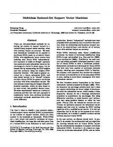
Figure 1. Working zones for a ν-K-SVCR in the feature space on a three-class problem.

to an example that is either misclassified or lying within the ρ-tube. Since our aim is to classify examples into multiple classes, we will modify the definition of margin errors. Namely, throughout this paper, the margin errors refer to two kinds of training examples: For the examples in the two classes to be separated, margin errors refer to the examples xi with ξi > 0, that is, the examples that are either misclassified or lying within the ρ-tube; for the examples that are not in either of the two classes, margin errors refer to the examples lying outside the ε-tube. Specifically, the margin errors are the training examples that belong to the set {i : yi g(xi ) < ρ, i = 1, · · · , l12 } ∪ {i : |g(xi )| > ε, i = l12 + 1, · · · , l},

(41)

where g(·) is defined by (38). Figure 1 depicts the working zones for a ν-K-SVCR in the feature space on a three-class problem: The ‘¦’, ‘◦’ and ‘∗’ represent the classes labelled by −1, +1 and 0 respectively. Examples with output −1: A, well-classified example (vi = 0); B, support vector (vi ∈ (− lC12 , 0)); X, margin error with label −1 (vi = − lC12 ) (X is regarded as a margin error since we have yi g(xi ) ≥ ρ for this example, even if it is labelled as −1, cf. (41)); Y, margin error with label 0 (vi = − lC12 ); Z, margin error with label +1 (vi = lC12 ). Examples with output +1: Similar to the above. Examples with output 0: E, well-classified example (vi = 0); F, support D vector (vi ∈ (0, D l3 )); G, support vector ( vi ∈ (− l3 , 0)); H, margin error (vi = −D l3 ). The fraction of margin errors is defined as the number of margin errors

10

P. ZHONG AND M. FUKUSHIMA

divided by the total number of examples, i.e., 1 {|{i : yi g(xi ) < ρ, i = 1, · · · , l12 }| + |{i : |g(xi )| > ε, i = l12 + 1, · · · , l}|} , l (42) where g(·) is defined by (38). FME :=

Theorem 3.1 Suppose ν-K-SVCR is applied to some data set, and the resulting ε and ρ satisfy ρ > ε > 0. Then the following statements hold: 2 l3 (i). ν1 l12 +ν is an upper bound on the fraction of margin errors. l ν1 l12 +ν2 l3 (ii). is a lower bound on the fraction of SVs. l (iii). Suppose the data are i.i.d. from a distribution P (x, θ) = P (x)P (θ|x) such that none of P (x, θ = Θ1 ), · · · , P (x, θ = ΘK ) contain any discrete component. Suppose that the kernel is analytic and non-constant. With probability 2 l3 1, asymptotically, ν1 l12 +ν equals both the fraction of SVs and the fraction of l margin errors. 12 Proof (i). Suppose the numbers of margin errors in examples {(xi , θi )}li=1 l and {(xi , θi )}i=l12 +1 are m1 and m2 , respectively. If an example belonging to l12 {(xi , θi )}i=1 is a margin error, then the corresponding slack variable satisfies ξi > 0, which along with (29) implies µi = 0. Hence by (21), the examples with ξi > 0 satisfy αi = lC12 . On the other hand, since ρ > ε, (33) yields ς = 0. Hence (24) becomes

l12 X

αi = Cν1 .

(43)

i=1 12 Therefore, at most ν1 l12 examples in {(xi , θi )}li=1 can have αi = obtain

m1 ≤ ν1 l12 .

C l12 .

Thus we

(44)

If an example belonging to {(xi , θi )}li=l12 +1 is a margin error, then the corresponding dual variables satisfy ϕi > 0 or ϕ˜i > 0. By (30) or (31), we have D ˜ ηi = 0 or η˜i = 0 correspondingly. By (22) and (23), we get βi = D l3 or βi = l3 . On the other hand, ρ > ε > 0 implies ζ = 0 and ς = 0. So (25) becomes l X

(βi + β˜i ) = Dν2 .

(45)

i=l12 +1

Since βi β˜i = 0, (45) implies that at most ν2 l3 examples in {(xi , θi )}li=l12 +1 can

A NEW MULTI-CLASS SUPPORT VECTOR ALGORITHM

have βi =

D l3

or β˜i =

D l3 .

11

Thus we obtain m2 ≤ ν2 l3 .

(46)

2 l3 Combining (44) and (46) shows that ν1 l12 +ν is an upper bound on the fracl tion of margin errors. 12 (ii). If an example belonging to {(xi , θi )}li=1 is a support vector, it can C contribute at most l12 to the left-hand side of (43). Hence there must be at least ν1 l12 SVs. Similarly, for the examples in {(xi , θi )}li=l12 +1 , by (45) and noting βi β˜i = 0, we can deduce that there must be at least ν2 l3 SVs. Therefore, ν1 l12 +ν2 l3 is an lower bound on the fraction of SVs. l (iii). We prove it by showing that, asymptotically, the probability of examples on the edges of ρ-tube or ε-tube (that is, the examples that satisfy yi g(xi ) = ρ, i = 1, · · · , l12 , or g(xi ) = ±ε, i = l12 + 1, · · · , l) vanishes. It follows from the condition on P (x, θ) that, apart from some set of measure zero, the K class distributions are absolutely continuous. Since the kernel is analytic and non-constant, it cannot be constant on any open set. Hence all the functions g constituting the argument of the sign in the decision function (cf. (37)) cannot be constant on any open set. Therefore, the distribution over x can be transformed into the distributions such that for all t ∈ R, limγ→0 P (|g(x) + t| < γ) = 0. On the other hand, since the class of these functions has well-behaved covering numbers, we get uniform convergence, i.e., for all γ > 0 and t ∈ R,

P sup |P (|g(x) + t| < γ) − Pˆl (|g(x) + t| < γ)| → 0, l → ∞, g

where Pˆl is the sample-based estimate of P with l being the sample size (that is, the proportion of examples that satisfy |g(x) + t| < γ). Then for any σ > 0 and any t ∈ R, we have lim lim P (sup Pˆl (|g(x) + t| < γ) > σ) = 0,

γ→0 l→∞

g

and hence P sup Pˆl (|g(x) + t| = 0) → 0, l → ∞. g

Setting t = ±ρ or t = ±ε shows that almost surely the fraction of examples exactly on the edges of ρ-tube or ε-tube tends to zero. Since SVs include the examples on the edges of ρ-tube or ε-tube and margin errors, the fraction of

12

P. ZHONG AND M. FUKUSHIMA

SVs equals that of margin errors. It then follows from (i) and (ii) that both 2 l3 fractions converge almost surely to ν1 l12 +ν . ¤ l Theorem 3.1 gives a theoretical bound on the fraction of margin errors. In fact, we will show in Section 4 by numerical experiments that this theoretical bound is practically useful in estimating the number of margin errors. For each classifier of ν-K-SVCR, the following theorem shows the ‘outlier’ resistance property. We use shorthand zi for φ(xi ) below. Theorem 3.2 Suppose w can be expressed in terms of the SVs that are not margin errors, that is, w=

l X

λi zi ,

(47)

i=1

where λi = 0 for all i ∈ / U := {i ∈ {1, · · · , l12 } : − lC12 < vi < 0 or 0 < S D vi < lC12 } {i ∈ {l12 + 1, · · · , l} : 0 < vi < D l3 or − l3 < vi < 0}. Then a sufficiently small perturbation of any margin error zm along the direction w does not change the hyperplane. Proof We first consider the case m ∈ {1, · · · , l12 }. Since the slack variable corresponding to zm satisfies ξm > 0, it follows from (29) that µm = 0. Then by (21) and (34), we get vm = lC12 or − lC12 . Let z0m := zm + ϑw, where |ϑ| is sufficiently small. Then the slack variable corresponding to z0m will still satisfy 0 > 0. Hence we have v 0 = v . Replacing ξ 0 ξm m m by ξm and keeping all other m primal variables unchanged, we obtain an updated vector of primal variables that is still feasible. In order to keep w unchanged, from the expression (35) of w, we need to let vi0 , i 6= m, satisfy l X i=1

vi zi =

X

vi0 zi + vm z0m .

(48)

i6=m

Substituting z0m = zm + ϑw and (47) into (48), and noting that m ∈ / U, we get a sufficient condition for (48) to hold is that for all i 6= m vi0 = vi − ϑλi vm .

(49)

We next show that b is also kept unchanged. Recall that by assumption λi = 0 0 = v , (49) yields for any i ∈ / U, and so λm = 0. Hence by (34) and vm m αi0 = αi − ϑλi yi αm ym ,

i = 1, · · · , l12 .

A NEW MULTI-CLASS SUPPORT VECTOR ALGORITHM

13

´ ³ ´ ³ If αi ∈ 0, lC12 , then αi0 will be in 0, lC12 , provided |ϑ| is sufficiently small. If αi = lC12 , then by assumption we have λi = 0, and hence αi0 will equal lC12 . Thus a small perturbation zm along the direction w does not change the status of examples (xi , θi ), i = 1, · · · , l12 . By (39), b does not change. Thus (w, b) remains to be the hyperplane parameters. In the case m ∈ {l12 + 1, · · · , l}, the result can be obtained in a similar way. ¤. The new learning machine makes the fusion of the standard structures, oneagainst-one and one-against-all, employed in the decomposition scheme of a multi-class classification procedure. In brief, a ν-K-SVCR classifier is trained to focus on the separation between two classes, as one-against-one does. At the same time, it also gives useful information about the other classes that are labelled 0, as one-against-all does. In addition, for each classifier, we can use the parameters ν1 and ν2 to control the number of margin errors, which is helpful in improving the accuracy of each classifier. Theorem 3.2 indicates that every classifier is robust. 3.3

The Connection to K-SVCR

Angulo et al. [2] propose K-SVCR method for the multi-class classification. The following theorem shows that ν-K-SVCR formulation will result in the same classifier as that of K-SVCR by selecting the parameters properly. Theorem 3.3 If wν , bν , ξiν , ϕνi , ϕ˜νi , εν and ρν > 0 constitute an optimal ν C = bν , ξ C = solution to a ν-K-SVCR with given ν1 , ν2 , then wC = w i ρν , b ρν ξiν ρν ,

ν

ν

ϕi ϕ ˜i ϕC ˜C i = ρν , ϕ i = ρν constitute an optimal solution to the corresponding Cν C = Dν and δ C = εν being a priori chosen K-SVCR, with C C = l12 ρν , D l3 ρν ρν parameters in K-SVCR.

Proof Consider the primal formulation of ν-K-SVCR. Let an optimal solution be given by wν , bν , ξiν , ϕνi , ϕ˜νi , εν and ρν . Substituting w0 = ρwν , b0 = ρbν ,

ξi0 = ρξνi , ϕ0i = ρϕνi and ϕ˜0i = optimization problem

ϕ ˜i ρν

in the ν-K-SVCR (13)–(18), we have the

l l X X 1 min{w0 ,b0 ,ξ0 ,ϕ0 ,ϕ˜0 } kw0 k2 + C C ξi0 + DC ( (ϕ0i + ϕ˜0i )) 2 i=1

s.t.

yi ((w0 · φ(xi )) + b0 ) ≥ 1 − ξi0 , i = 1, · · · , l12 , C

−δ − ϕ˜0i ≤ (w0 ξi0 , ϕ0i , ϕ˜0i ≥ 0.

0

(50)

i=1

C

· φ(xi )) + b ≤ δ +

ϕ˜0i ,

i = l12 + 1, · · · , l,

(51) (52) (53)

14

P. ZHONG AND M. FUKUSHIMA

Note that this has the same form as K-SVCR. It is not difficult to see that wC , bC , ξiC , ϕC ˜C i , ϕ i constitute an optimal solution to problem (50)–(53). ¤ 3.4

The Combination Method

After the decomposition scheme, we need a reconstruction scheme to fuse the outputs of all classifiers for each example and assign it to one of the classes. In a K-class problem, for each pair, say Θj and Θk , we have a classifier fj,k (·) to separate them as well as the other classes (cf.(12)). So we have K(K − 1)/2 classifiers in total. Hence, for an example xp , we get K(K − 1)/2 outputs. We translate the outputs as follows: When fj,k (xp ) = +1, a positive vote is added on Θj , and no votes are added on the other classes; when fj,k (xp ) = −1, a positive vote is added on Θk , and no votes are added on the other classes; when fj,k (xp ) = 0, a negative vote is added on both Θj and Θk , and no votes are added on the other classes. After we translate all of the K(K − 1)/2 outputs, we will get the total votes of each class by adding the positive and negative votes on this class. Finally, xp will be assigned to the class that gets the most votes.

4

EXPERIMENTS

In this section, we present two types of experiments demonstrating the performance of ν-K-SVCR: Experiments on artificial data sets which are used to verify the theoretical results, and experiments on benchmark data sets.

4.1

Experiments on Artificial Data Sets

In this subsection, several experiments with artificial data in R2 are carried out using Matlab v6.5 on Intel Pentium IV 3.00GHz PC with 1GB of RAM. The QP problems are solved with the standard Matlab routine. For simplicity, we set ν1 = ν2 , which is denoted ν. The main tasks in the experiments are the following: (1) To investigate the effect of parameter ν on the fraction of margin errors, the fraction of SVs, and the values of ε and ρ; (2) To observe an asymptotic behavior of the fractions of margin errors and SVs. The effect of parameter ν The influence of parameter ν is investigated on the training set T generated from a Gaussian distribution on R2 . The set T contains 150 examples in three classes, each of which has 50 examples, as shown in Figure 2.

A NEW MULTI-CLASS SUPPORT VECTOR ALGORITHM

15

Figure 2. Training set T

Table 1. Fractions of margin errors and SVs and the values of ε and ρ for T .

ν FMEa FSVb ε ρ

0.1

0.2

0.3

0.4

0.5

0.6

0.7

0.8

0 0.3867 0.0246 14.2287

0.0667 0.4067 0.0112 29.1982

0.1667 0.5333 0.0085 49.2638

0.2667 0.6133 0.0045 72.9279

0.3533 0.6867 0.0041 100.2379

0.4600 0.7867 0.0009 131.1074

0.5600 0.8333 0.0005 166.9139

0.6400 0.8933 0 213.3048

a Fraction

of margin errors.

b Fraction

of support vectors.

In the experiment, a Gaussian kernel with σ = 0.2236 is employed. We choose C = 2000 and D = 300. Table 1 shows that ν provides an upper bound of the fraction of margin errors and a lower bound of the fraction of SVs, and that increasing ν allows more margin errors, increases the value of ρ, and decreases the value of ε. It is worth noticing from Table 1 that the assumption ρ > ε in Theorem 3.1 does hold in practice. The tendency of the fractions of margin errors and SVs In this experiment, we show the tendency of the fractions of margin errors and SVs when the number of training examples increases. We choose ν = 0.2. Ten training sets are generated from the same Gaussian distribution. In each training set, there are three classes. The total number of examples in each 2 l3 training set is l, and each class has l/3 examples. Hence we have ν1 l12 +ν = l 0.2. We use a polynomial kernel with degree 4, and set C = 100, D = 50. Table 2 shows that both the fraction of margin errors and the fraction of SVs tend to 0.2 from below and above, respectively, when the total number of examples l increases. This confirms the results established in Theorem 3.1.

16

P. ZHONG AND M. FUKUSHIMA Table 2.

Asymptotic behavior of the fractions of margin errors and SVs.

l

30

60

90

120

150

180

210

240

270

300

0.13 0.30

0.13 0.25

0.18 0.23

0.17 0.22

0.18 0.22

0.19 0.23

0.19 0.22

0.19 0.22

0.19 0.21

0.20 0.20

FME FSV

Table 3. The percentage of error by 1-a-a, 1-a-1, qp-mc-sv, lp-mc-sv, K-SVCR and ν-K-SVCR.

name

#ptsa

#attb

#class

1-a-a

1-a-1

qp-mc-sv

lp-mc-sv

K-SVCR

ν-K-SVCR

Iris Wine Glass

150 178 214

4 13 9

3 3 6

1.33 5.6 35.2

1.33 5.6 36.4

1.33 3.6 35.6

2.0 10.8 37.2

[1.93, 3.0] [2.29, 4.29] [30.47, 36.35]

1.33 3.3 [32.38, 36.19]

a

The number of training data.

b

The attributes of examples.

4.2

Experiments on Benchmark Data Sets

In this subsection, we test ν-K-SVCR on a collection of three benchmark data sets from the UCI machine learning repository [4], ‘Iris’, ‘Wine’ and ‘Glass’. In problem ‘Glass’, there is one missing class. Since no test data sets are provided in the three benchmark data sets, we use ten-fold cross validation to evaluate the performance of the algorithms. That is, each data set is split randomly into ten subsets and one of those sets is reserved as a test set; this process is repeated ten times. For ‘Iris’ and ‘Wine’, the polynomial kernels with degree 4 and 3 are employed, respectively. For ‘Glass’, the Gaussian kernel with σ = 0.2236 is employed. We choose ν = 0.01 in each algorithm. We compare the obtained results with one-against-all (1-a-a), one-against-one (1-a-1), quadratic multi-class SVM (qp-mc-sv) and linear multi-class SVM (lp-mc-sv) proposed in [23], and K-SVCR proposed in [2]. The results are summarized in Table 3. In the table, [·, ·] refers to the case where two or more classes get the most votes in a tie. The first and second numbers in the brackets are the percentage of error when examples are assigned to the right and the wrong classes, respectively, among those with the most votes. It can be observed that the performance of the new algorithm is generally comparable to the other ones. Specifically, for the ‘Iris’ set, ν-K-SVCR outperforms the lp-mc-sv and K-SVCR methods; and it is comparable to the others. For the ‘Wine’ set, ν-K-SVCR is comparable to K-SVCR; and it outperforms the others. For the ‘Glass’ set, ν-K-SVCR shows a similar performance to all the others. Note that the new algorithm is not fundamentally different from the K-SVCR algorithm. Indeed, we have shown that for a certain parameter setting, both algorithms will produce the same results. In practice, however, it may sometimes be desirable to specify a fraction of points that are allowed to become errors.

A NEW MULTI-CLASS SUPPORT VECTOR ALGORITHM

5

17

CONCLUSION

We have proposed a new algorithm, ν-K-SVCR, for the multi-class classification based on ν-SV classification and ν-SV regression. By redefining the concept of margin errors, we have clarified the theoretical meaning of the parameters in ν-K-SVCR. We have also shown the robustness of the classifiers and connection to K-SVCR. We have confirmed the established theoretical results and good behavior of the algorithm through experiments on several artificial data and benchmark data sets. Future research subjects include more comprehensive testing of the algorithm and application to real-world problems.

References [1] E. L. Allwein, R. E. Schapire and Y. Singer (2001). Reducing multiclass to binary: A unifying approach for margin classifiers. Journal of Machine Learning Research, 1, 113–141. [2] C. Angulo, X. Parra and A. Catal` a (2003). K-SVCR. A support vector machine for multi-class classification. Neurocomputing, 55, 57–77. [3] K.P. Bennett (1999). Combining support vector and mathematical programming methods for classification. in: B. Sch¨ olkopf, C. J. C. Burges and A. J. Smola (Eds.), Advances in Kernel Methods: Support Vector Learning, pp. 307–326. MIT Press, Cambridge, MA. [4] C. L. Blake and C. J. Merz (1998). UCI repository of machine learning databases. University of California. [www http://www.ics.uci.edu/∼mlearn/MLRepository.html] [5] L. Bottou, C. Cortes, J. S. Denker, H. Drucker, I. Guyon, L. D. Jackel, Y. LeCun, U. A. M¨ uller, E. Sackinger, P. Simard and V. Vapnik (1994). Comparison of classifier methods: a case study in handwriting digit recognition. in: IAPR (Ed.), Proceedings of the International Conference on Pattern Recognition, pp. 77–82. IEEE Computer Society Press. [6] K. Crammer and Y. Singer (2002). On the algorithmic implementation of multiclass kernel-basd vector machines. Journal of Machine Learning Research, 2, 265–292. [7] K. Crammer and Y. Singer (2002). On the learnability and design of output codes for multiclass problems. Machine Learning, 47, 201–233. [8] N. Cristianini and J. Shawe-Taylor (2000). An Introduction to Support Vector Machines. Cambridge University Press, Cambridge, UK. [9] T.G. Dietterich and G. Bakiri (1995). Solving multi-class learning problems via error-correcting output codes. Journal of Artificial Intelligence Research, 2, 263–286. [10] J. F¨ urnkranz (2002). Round robin classification. Journal of Machine Learning Research, 2, 721– 747. [11] T. J. Hastie and R. J. Tibshirani (1998). Classification by pairwise coupling. in: M. I. Jordan, M. J. Kearns and S. A. Solla (Eds.), Advances in Neural Information Processing Systems, 10, 507–513. MIT Press, Cambridge, MA. [12] U. Kreßel (1999). Pairwise classification and support vector machines. in: B. Sch¨ olkopf, C. J. C. Burges and A. J. Smola (Eds.), Advances in Kernel Methods: Support Vector Learning, pp. 255–268. MIT Press, Cambridge, MA. [13] C. W. Hsu and C. J. Lin (2002). A comparison of methods for multiclass support vector machines. IEEE Transactions on Neural Networks, 13, 415–425. [14] Y. Lee, Y. Lin and G. Wahba (2001). Multicategory support vector machines. Computing Science and Statistics, 33, 498–512. [15] J. Mercer (1909). Functions of positive and negative type and their connection with the theory of integral equations. Philosophical Transactions of the Royal Society, London, A 209, 415–446. [16] M. Moreira and E. Mayoraz (1998). Improved pairwise coupling classification with correcting classifiers. Lecture Notes in Computer Science: Proceedings of the 10th European conference on Machine Learning, pp. 160–171. [17] J. Platt (1999). Probabilistic outputs for support vector machines and comparisons to regularized likelihood methods. in: A.J. Smola, P. Bartlett, B. Sch¨ olkopf and D. Schuurmans (Eds.), Advances in Large Margin Classifiers, pp. 61–74. MIT Press, Cambridge, MA. [18] J. Platt, N. Cristianini and J. Shawe-Taylor (2000). Large margin DAGs for multiclass classifi-

18

[19] [20] [21] [22] [23]

P. ZHONG AND M. FUKUSHIMA cation. in: S. A. Solla, T. K. Leen and K. -R. M¨ uller (Eds.), Advances in Neural Information Processing Systems, 12, 547–553. MIT Press, Cambridge, MA. R. Rifkin and A. Klautau (2004). In defense of one-vs-all classification. Journal of Machine Learning Research, 5, 101–141. B. Sch¨ olkopf, A. J. Smola, R. C. Williamson and P. L. Bartlett (2000). New support vector algorithms. Neural Computation, 12, 1207–1245. V. Vapnik (1995). The Nature of Statistical Learning Theory. Springer-Verlag, New York. V. Vapnik (1998). Statistical Learning Theory. Wiley, New York. J. Weston and C. Watkins (1998). Multi-class support vector machines. CSD-TR-98-04 Royal Holloway, University of London, Egham, UK.