A Simulated Annealing Algorithm to Construct Covering Perfect Hash

Hindawi Mathematical Problems in Engineering Volume 2018, Article ID 1860673, 14 pages https://doi.org/10.1155/2018/1860673

Research Article A Simulated Annealing Algorithm to Construct Covering Perfect Hash Families Jose Torres-Jimenez

and Idelfonso Izquierdo-Marquez

CINVESTAV-Tamaulipas, Cd. Victoria 87130, Tamaulipas, Mexico Correspondence should be addressed to Jose Torres-Jimenez; [email protected] Received 27 January 2018; Accepted 29 May 2018; Published 26 July 2018 Academic Editor: Fiorenzo A. Fazzolari Copyright © 2018 Jose Torres-Jimenez and Idelfonso Izquierdo-Marquez. This is an open access article distributed under the Creative Commons Attribution License, which permits unrestricted use, distribution, and reproduction in any medium, provided the original work is properly cited. Covering perfect hash families (CPHFs) are combinatorial designs that represent certain covering arrays in a compact way. In previous works, CPHFs have been constructed using backtracking, tabu search, and greedy algorithms. Backtracking is convenient for small CPHFs, greedy algorithms are appropriate for large CPHFs, and metaheuristic algorithms provide a balance between execution time and quality of solution for small and medium-size CPHFs. This work explores the construction of CPHFs by means of a simulated annealing algorithm. The neighborhood function of this algorithm is composed of three perturbation operators which together provide exploration and exploitation capabilities to the algorithm. As main computational results we have the generation of 64 CPHFs whose derived covering arrays improve the best-known ones. In addition, we use the simulated annealing algorithm to construct quasi-CPHFs from which quasi covering arrays are derived that are then completed and postoptimized; in this case the number of new covering arrays is 183. Together, the 247 new covering arrays improved the upper bound of 683 covering array numbers.

1. Introduction A covering arrayCA(𝑁; 𝑡, 𝑘, V) of strength 𝑡 is an 𝑁 × 𝑘 array over the symbol set ZV = {0, 1, . . . , V − 1} such that in every 𝑁 × 𝑡 subarray all 𝑡-tuples over ZV occur at least once. If each 𝑡-tuple over ZV occurs exactly once in every 𝑁 × 𝑡 subarray, then the array is an orthogonal array of strength 𝑡, denoted by OA(𝑁; 𝑡, 𝑘, V). Every orthogonal array is a covering array, but not every covering array is an orthogonal array. The main applications of covering arrays are in software and hardware testing. In the testing strategy called combinatorial testing, covering arrays are viewed as test-suites where the strength 𝑡 is the size of the interactions to be checked in a software component. For example, a covering array of strength 𝑡 = 3 can be used to test all possible combinations of values among any three of the 𝑘 parameters; see [1] for an introduction to the use of covering arrays in combinatorial testing. In the area of hardware testing, covering arrays have been used to check the presence of hardware Trojans [2]. Given the values of the strength 𝑡, the number of columns 𝑘, and the order V, the problem of constructing covering arrays is the problem of finding the minimum number of

rows 𝑁 such that a CA(𝑁; 𝑡, 𝑘, V) exists. Currently, there is no polynomial-time algorithm to solve optimally this problem for general values of 𝑡, 𝑘, and V; only some particular cases have been solved optimally [3–6]. The smallest 𝑁, for which a covering array exists with strength 𝑡, 𝑘 columns, and order V, is called the covering array number of 𝑡, 𝑘, V, and it is denoted by CAN(𝑡, 𝑘, V). A trivial lower bound for the covering array number is CAN(𝑡, 𝑘, V) ≥ V𝑡 , since every subarray of 𝑡 columns must cover every one of the V𝑡 possible 𝑡-tuples over the V symbols. In addition to the cases with optimal solution, a number of improvements in the lower bounds for specific cases have been reported in [7–9]. With regard to upper bounds, much work has been done to constantly improve them, and several algorithms have been developed to construct increasingly better covering arrays. To keep track of the advances in the construction of covering arrays, the Covering Array Tables [10] contain the current best-known upper bounds for strengths 2 ≤ 𝑡 ≤ 6 and orders 2 ≤ V ≤ 25. The techniques used to construct covering arrays can be classified as exact, greedy, metaheuristic, algebraic, and

2 recursive; see [11–14] for an overview of covering array construction methods. Metaheuristic algorithms to construct covering arrays include tabu search [15], genetic algorithms [16], simulated annealing [17], ant colony [18], particle swarm optimization [19], harmony search [20], hill climbing [21], bird swarm [22], a combination of bee colony and harmony search [23], Cuckoo search [24], differential evolution [25], tabu search as a hyperheuristic [26], and a combination of simulated annealing with a greedy algorithm [27]. One way to construct covering arrays is to use a high level representation of them called covering perfect hash family (CPHF). The elements of a CPHF are (𝑡 − 1)-tuples or 𝑡-tuples over ZV that represent a column vector of length V𝑡 . CPHFs are a compact representation of covering arrays because a CPHF with 𝑛 rows and 𝑘 columns represents a covering array with 𝑛V𝑡 rows and 𝑘 columns. Commonly CPHFs have few rows (say 𝑛 ≤ 20), but their corresponding covering arrays may have a large number of rows depending on the values of V and 𝑡. In this work we develop a simulated annealing (SA) algorithm to construct CPHFs. The neighborhood function of the SA algorithm is composed of three perturbation operators which together provide exploration and exploitation capabilities to the SA algorithm. The probability of using one of the three operators in an application of the neighborhood function is tuned by experimenting with a number of probability distributions. Relevant results obtained with the SA algorithm are 64 new CPHFs whose respective covering arrays improved the best-known ones and other 183 new covering arrays obtained by means of a procedure based on constructing quasi-CPHFs. In total, these 64+183 = 247 new covering arrays improve the upper bound of 683 covering array numbers CAN(𝑡, 𝑘, V). This paper is organized as follows: Section 2 provides a background on CPHFs; Section 3 reviews some related works; Section 4 describes the components of the SA algorithm and shows the experimentation done to set the utilization rate of the operators in the neighborhood function; Section 5 presents the computational results; and Section 6 gives the conclusions of the work.

2. Covering Perfect Hash Families CPHFs were introduced by Sherwood et al. [28]. Let V be a prime power and let FV denote the finite fields with V elements. (𝑖) For a given strength 𝑡, let (𝛽0(𝑖) , 𝛽1(𝑖) , . . . , 𝛽𝑡−1 ) be the base V (𝑖) 𝑡 𝑗 representation of 𝑖 ∈ {0, 1, . . . , V − 1}; that is, 𝑖 = ∑𝑡−1 𝑗=0 V ⋅ 𝛽𝑗 . 󳨀󳨀󳨀󳨀󳨀󳨀󳨀󳨀󳨀󳨀󳨀󳨀󳨀󳨀→ As defined in [28], a permutation vector (ℎ1 , ℎ2 , . . . , ℎ𝑡−1 ) is the vector of length V𝑡 that has the symbol 𝛽0(𝑖) + (ℎ1 × 𝛽1(𝑖) ) + (𝑖) (ℎ2 × 𝛽2(𝑖) ) + ⋅ ⋅ ⋅ + (ℎ𝑡−1 × 𝛽𝑡−1 ) in position 𝑖 for 0 ≤ 𝑖 ≤ V𝑡 − 1. Permutation vectors are vectors with V𝑡 elements from FV , but they are represented by (𝑡 − 1)-tuples over FV . For fixed V and 𝑡 the number of distinct permutation vectors is V𝑡−1 . The term “permutation vector” is because the vectors of length V𝑡 are formed by concatenating V𝑡−1 permutations of (0, 1, . . . , V − 1). For example, Table 1 shows the V𝑡−1 = 32 = 9 distinct permutation vectors for V = 3 and 𝑡 = 3.

Mathematical Problems in Engineering Table 1: Permutation vectors for V = 3 and 𝑡 = 3. Starting from the first element, every group of V = 3 elements is a permutation of (0, 1, 2). Perm Vec 󳨀󳨀󳨀→ (0, 0) (0 󳨀󳨀󳨀→ (0, 1) (0 󳨀󳨀󳨀→ (0, 2) (0 󳨀󳨀󳨀→ (1, 0) (0 󳨀󳨀󳨀→ (1, 1) (0 󳨀󳨀󳨀→ (1, 2) (0 󳨀󳨀󳨀→ (2, 0) (0 󳨀󳨀󳨀→ (2, 1) (0 󳨀󳨀󳨀→ (2, 2) (0

Elements 1 2 0 1 2 0 1 2 0 1 2 0 1 2 0 1 2 0 1 2 0 1 2 0 1 2) 1 2 0 1 2 0 1 2 1 2 0 1 2 0 1 2 0 2 0 1 2 0 1 2 0 1) 1 2 0 1 2 0 1 2 2 0 1 2 0 1 2 0 1 1 2 0 1 2 0 1 2 0) 1 2 1 2 0 2 0 1 0 1 2 1 2 0 2 0 1 0 1 2 1 2 0 2 0 1) 1 2 1 2 0 2 0 1 1 2 0 2 0 1 0 1 2 2 0 1 0 1 2 1 2 0) 1 2 1 2 0 2 0 1 2 0 1 0 1 2 1 2 0 1 2 0 2 0 1 0 1 2) 1 2 2 0 1 1 2 0 0 1 2 2 0 1 1 2 0 0 1 2 2 0 1 1 2 0) 1 2 2 0 1 1 2 0 1 2 0 0 1 2 2 0 1 2 0 1 1 2 0 0 1 2) 1 2 2 0 1 1 2 0 2 0 1 1 2 0 0 1 2 1 2 0 0 1 2 2 0 1)

Another characteristic of permutation vectors is that their first V elements are 0, 1, . . . , V − 1 in that order. Given a tuple of 𝑡 permutation vectors, let 𝐴 be the array of size V𝑡 × 𝑡 whose columns are the 𝑡 permutation vectors of the tuple. If 𝐴 is an OA(V𝑡 ; 𝑡, 𝑡, V) then the 𝑡tuple of permutation vectors is covering; otherwise the 𝑡tuple is noncovering. For example, the 3-tuple of permutation 󳨀󳨀󳨀→ 󳨀󳨀󳨀→ 󳨀󳨀󳨀→ vectors ((0, 2), (1, 0), (1, 1)) is covering, because we can verify 󳨀󳨀󳨀→ in Table 1 that the array of size 27 × 3 with columns (0, 2), 󳨀󳨀󳨀→ 󳨀󳨀󳨀→ (1, 0), and (1, 1) is an OA(27; 3, 3, 3). On the other hand, the 󳨀󳨀󳨀→ 󳨀󳨀󳨀→ 󳨀󳨀󳨀→ tuple ((0, 0), (0, 1), (0, 2)) is noncovering since we can see in Table 1 that the array formed by the permutation vectors of the tuple is not an orthogonal array. A CPHF(𝑛; 𝑘, V𝑡−1 , 𝑡) is an 𝑛 × 𝑘 array with elements from 𝑡−1 FV such that every subarray of 𝑡 columns has at least one row that is a covering tuple of 𝑡 permutation vectors [28]. A CPHF(𝑛; 𝑘, V𝑡−1 , 𝑡) generates a CA(𝑛(V𝑡 ); 𝑡, 𝑘, V) replacing the elements of the CPHF by the corresponding permutation vectors of length V𝑡 . However, since the first V elements of every permutation vector are (0, 1, . . . , V − 1), it is possible to delete the first V elements from every permutation vector given by the last 𝑛 − 1 rows of the CPHF; the result is a CA(𝑛(V𝑡 − V) + V; 𝑡, 𝑘, V). Equation (1) shows a CPHF(3; 15, 52 , 3); the 󳨀󳨀󳨀󳨀󳨀󳨀→ permutation vectors (ℎ1 , ℎ2 ) are written as ℎ1 ℎ2 . Every one of the ( 15 3 ) subarrays of 𝑡 = 3 columns contains as a row a covering tuple of permutation vectors. This CPHF generates a CA(365; 3, 15, 5). Example of a 𝐶𝑃𝐻𝐹(3; 15, 52 , 3) 11 00 02 01 20 03 34 23 24 13 31 44 40 41 33 (23 01 21 04 12 40 44 01 14 22 44 02 31 41 30) (1) 21 04 30 30 13 01 40 02 31 41 21 12 55 43 03

In addition to permutation vectors generated by a (𝑡 − 1)tuple over FV , we have that a 𝑡-tuple (ℎ0 , ℎ1 , . . . , ℎ𝑡−1 ) over FV also generates a vector of V𝑡 elements when evaluated as (𝑖) (ℎ0 × 𝛽0(𝑖) ) + (ℎ1 × 𝛽1(𝑖) ) + ⋅ ⋅ ⋅ + (ℎ𝑡−1 × 𝛽𝑡−1 ) in the base V (𝑖) (𝑖) (𝑖) representation (𝛽0 , 𝛽1 , . . . , 𝛽𝑡−1 ) of every 0 ≤ 𝑖 ≤ V𝑡 − 1. However, some of these 𝑡-tuples (ℎ0 , ℎ1 , . . . , ℎ𝑡−1 ) generate

Mathematical Problems in Engineering Table 2: Example of extended permutation vectors for V = 3 and 𝑡 = 3. E. Perm Vec 󳨀󳨀󳨀󳨀󳨀󳨀→ (0, 0, 1) 󳨀󳨀󳨀󳨀󳨀󳨀→ (0, 2, 1) 󳨀󳨀󳨀󳨀󳨀󳨀→ (1, 0, 1) 󳨀󳨀󳨀󳨀󳨀󳨀→ (1, 1, 2) 󳨀󳨀󳨀󳨀󳨀󳨀→ (2, 0, 1) 󳨀󳨀󳨀󳨀󳨀󳨀→ (2, 1, 2)

Elements (0 0 0 0 0 0 0 0 0 1 1 1 1 1 1 1 1 1 2 2 2 2 2 2 2 2 2) (0 0 0 2 2 2 1 1 1 1 1 1 0 0 0 2 2 2 2 2 2 1 1 1 0 0 0) (0 1 2 0 1 2 0 1 2 1 2 0 1 2 0 1 2 0 2 0 1 2 0 1 2 0 1) (0 1 2 1 2 0 2 0 1 2 0 1 0 1 2 1 2 0 1 2 0 2 0 1 0 1 2) (0 2 1 0 2 1 0 2 1 1 0 2 1 0 2 1 0 2 2 1 0 2 1 0 2 1 0) (0 2 1 1 0 2 2 1 0 2 1 0 0 2 1 1 0 2 1 0 2 2 1 0 0 2 1)

vectors that are not permutation vectors; specifically, the 𝑡tuples with ℎ0 = 0 generate vectors of length V𝑡 , where every group of V elements is formed by V occurrences of the same symbol. 󳨀󳨀󳨀󳨀󳨀󳨀󳨀󳨀󳨀󳨀󳨀󳨀󳨀󳨀→ An extended permutation vector(ℎ0 , ℎ1 , . . . , ℎ𝑡−1 ) is 𝑡 defined as the vector of length V that has the symbol (𝑖) (ℎ0 × 𝛽0(𝑖) ) + (ℎ1 × 𝛽1(𝑖) ) + ⋅ ⋅ ⋅ + (ℎ𝑡−1 × 𝛽𝑡−1 ) in position 𝑖 for 0 ≤ 𝑡 𝑖 ≤ V − 1 [29]. For given V and 𝑡, the total number of extended permutation vectors is V𝑡 . As examples of extended permutation vectors, Table 2 shows six of the V𝑡 = 33 = 27 extended permutation vectors for V = 3 and 𝑡 = 3. Extended permutation vectors enlarge the available options to construct CPHFs, because the number of possible symbols is now V𝑡 . As for permutation vectors, a CPHF(𝑛; 𝑘, V𝑡 , 𝑡) generates a covering array replacing the elements of the CPHF by their corresponding extended permutation vectors of length V𝑡 . However, in this case it is not possible to delete the first V elements of the extended permutation vectors given by the last 𝑛 − 1 rows of the CPHF; only the first element can be deleted because it is zero in any extended permutation vector. Thus, a CPHF(𝑛; 𝑘, V𝑡 , 𝑡) generates a CA(𝑛(V𝑡 − 1) + 1; 𝑡, 𝑘, V) [29]. To make a distinction between CPHFs with elements from FV𝑡−1 and CPHFs with elements from FV𝑡 , we follow the convention of Colbourn et al. [30], where the first kinds of CPHFs are called Sherwood-CPHFs or SCPHFs, and the second ones are called simply CPHFs. For the same number of columns 𝑘 and the same number of rows 𝑛 > 1, a SCPHF(𝑛; 𝑘, V𝑡−1 , 𝑡) is better than a CPHF(𝑛; 𝑘, V𝑡 , 𝑡), because the SCPHF produces a covering array with less rows. However, CPHFs may have more columns than SCPHFs since there are more extended permutation vectors than permutation vectors.

3. Related Works This section reviews some methods to construct SCPHFs and CPHFs, and some SA algorithms to construct covering arrays. 3.1. Methods to Construct CPHFs. CPHFs were introduced by Sherwood et al. [28]. In that work SCPHFs were constructed by a backtracking algorithm. The first step of the algorithm is to initialize a candidate array of size 𝑛 × 𝑘; in this candidate array each entry takes its first valid element from FV𝑡−1 , but not

3 all entries of the candidate array have the same set of valid elements due to the following constraints: (1) If 𝑘 < V𝑡−1 the elements of the first row are in ascending order, and all elements are distinct. The other 𝑛 − 1 rows contain any permutation of FV𝑡−1 .

(2) If 𝑘 ≥ V𝑡−1 the array is divided into subarrays with at most V𝑡−1 columns; in each subarray every row has distinct elements from FV𝑡−1 , and the first row of each subarray has the 𝑖th element of FV𝑡−1 in its 𝑖th column. Once a candidate array is formed, i.e., all its entries are assigned with an element from FV𝑡−1 , the array is tested to see if it is a SCPHF. The test consists in verifying that every subarray of 𝑡 columns contains a covering tuple of permutation vectors. The following candidate arrays are generated using backtracking on the elements assigned to each entry of the array. This backtracking technique is only effective for a small number of columns, say 𝑘 ≤ 50, since the number of candidate arrays grows considerably with each new column. The authors report SCPHFs with up to 𝑘 = 44 columns for strength 𝑡 = 3, and with 𝑘 = 16 columns for strength four. Walker II and Colbourn [31] constructed SCPHFs using tabu search. The initial solution is an array of size 𝑛 × 𝑘 generated randomly. The algorithm employs a tabu list to store the last 50000 moves performed by the algorithm. A move replaces the value of one entry of the current solution by another value. Moves are only done in columns that are part of subarrays of 𝑡 columns with no covering tuple; such subarrays are called “uncovered subarrays”. The reason to restrict moves is that moves in columns that are not part of uncovered subarrays cannot improve the “score” of the current array. The score of the current solution is the number of subarrays with no covering tuple; when the score becomes zero a SCPHF has been obtained. The neighborhood of the current solution is all possible moves in all columns that are part of an uncovered subarray. At the beginning of the execution, the size of the neighborhood can be very large, and for this reason the neighborhood is restricted to the column that appears in more uncovered subarrays; such column is the worst column of the current solution. As the algorithm executes, the number of columns that belong to an uncovered subarray decreases and so the restriction of only considering the worst column is removed. The tabu search algorithm was able to construct SCPHFs with up to 255 columns for strength three, 62 columns for strength four, 19 columns for strength five, 14 columns for strength six, and 13 columns for strength seven. Recently Colbourn et al. [30] constructed SCPHFs and CPHFs by combining randomized and greedy algorithms. Firstly, a column resampling algorithm generates an initial CPHF (or SCPHF) and then a greedy algorithm adds new columns to the CPHF. The column resampling algorithm works as follows: the initial array of size 𝑛 × 𝑘 is generated by assigning its entries randomly; then, all subarrays of 𝑡 columns are checked to see if they are “covered”, that is if they have a covering tuple as a row. From each uncovered subarray one column is selected and its entries are reassigned with

4 random elements to try to decrease the number of uncovered subarrays. Columns are resampled until all subarrays are covered. After generating the initial CPHF, a greedy algorithm adds new columns to the CPHF. For each new column the algorithm generates randomly a number of candidates columns; if one of these candidates does not introduce uncovered subarrays then it is appended to the current CPHF, which now has one more column. If none candidate column can be appended to the CPHF without introducing uncovered subarrays, then one of the candidate columns replaces one of the current columns if there is one current column that is part of all uncovered subarrays introduced by the candidate column. This is a greedy strategy to replace the column most likely to participate in uncovered subarrays. By means of the combination of the column resampling algorithm and the greedy random extension algorithm, the authors constructed a great number of new SCPHFs and CPHFs whose corresponding covering arrays established a new upper bound of CAN(𝑡, 𝑘, V). Sizes of the SCPHFs and CPHFs constructed are 𝑘 = 10000 columns for strength three, 𝑘 = 2500 for strength four, 𝑘 = 600 for strength five, and 𝑘 = 200 for strength six. It is very difficult for a metaheuristic algorithm to construct CPHFs of these sizes in a reasonable amount of time. Then, our simulated annealing algorithm concentrates in small and medium-size CPHFs (𝑘 ≤ 50 and 50 < 𝑘 ≤ 350, respectively); we consider CPHFs with 𝑘 > 350 columns as large CPHFs. 3.2. SA Algorithms to Construct Covering Arrays. The SA technique has been used many times to find new upper bounds of CAN(𝑡, 𝑘, V). One of the most successful algorithms is the augmented annealing algorithm developed by Cohen et al. [32]. In that work the target covering array is divided into smaller arrays or “ingredients” using a combinatorial construction; after that, each ingredient is constructed either by a combinatorial technique or by SA if there is no combinatorial construction to generate the ingredient. Other work that uses SA is the one by Torres-Jimenez and Rodriguez-Tello [17]. In this SA algorithm only binary (V = 2) covering arrays are constructed. The initial solution is created randomly, but in such a way the symbols are balanced in each column; that is, there are ⌊𝑁/2⌋ zeros and 𝑁 − ⌊𝑁/2⌋ ones in every column. To generate a new solution from the current one the algorithm uses one of two relatively simple neighborhood functions 𝑁1 and 𝑁2 . The function 𝑁1 employs a procedure called switch (𝐴, 𝑖, 𝑗) that changes an entry of the current solution from 0 to 1, or from 1 to 0. The function 𝑁2 uses a procedure called swap (𝐴, 𝑖, 𝑗, 𝑙) to interchange the elements in the rows 𝑖 and 𝑙 of the column 𝑗. Avila-George et al. [33] developed three parallel SA algorithms called, respectively, independent search, semiindependent search, and cooperative search. In the independent search each processes runs an instance of the SA algorithm independently of the others; at the end, the best solution among all processes is taken as the final solution of the parallel SA algorithm. On the other hand, in the

Mathematical Problems in Engineering semi-independent search the processes exchange intermediate solutions in a synchronous way. After a predefined number of applications of the neighborhood function the processes share their best solution to select a global winner which is communicated to all processes, in order for all of them to know the current best global solution. In the cooperative search the processes share their current best solutions asynchronously. The SA algorithms developed so far to construct covering arrays work directly in the domain of covering arrays; that is, to construct a CA(𝑁; 𝑡, 𝑘, V) they work with matrices of size 𝑁 × 𝑘 over ZV , or with parts of the matrix as in the augmented annealing technique [32]. On the other hand, the SA algorithm developed in this work constructs the CAs in the domain of CPHFs, which is a high level representation of some covering arrays. Covering arrays and CPHFs are two distinct combinatorial objects; in covering arrays the requirement is that every subarray of 𝑡 columns contains at least once 𝑡-tuple over ZV , while in CPHFs the requirement is that every subarray of 𝑡 columns contains at least one covering tuple of permutation vectors. Then, although the structure of the SA algorithms proposed in this work may be similar to the structure of the SA algorithms developed to construct covering arrays, the neighborhood functions are different.

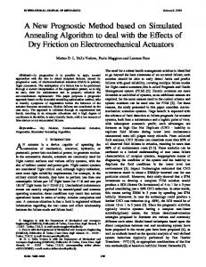
4. Simulated Annealing Algorithm This section describes the SA algorithm to construct SCPHFs and CPHFs. Section 4.1 shows the general structure of the SA algorithm. Section 4.2 presents the operators that form the neighborhood function and describes the experimentation done to find the more convenient values for the utilization rate of each operator. Section 4.3 reviews the noncovering test of [28, 31] to determine efficiently if a tuple of permutation vectors is noncovering; also this subsection describes how the noncovering test is adapted to extended permutation vectors. 4.1. Structure of the SA Algorithm. Simulated annealing is a metaheuristic inspired in the process of heating and cooling metals to obtain a strong crystalline structure. A metal is heated until it melts and then it is cooled in a controlled way. At the end of the process, the particles of the metal are arranged in such a way the energy of the system is minimal [34]. The evolution of the metal from melted to ground state is simulated as follows: given a current solution 𝑥 with energy 𝐸𝑥 ; from a perturbation of 𝑥 a new solution 𝑦 with energy 𝐸𝑦 is created. If 𝐸𝑦 < 𝐸𝑥 then 𝑦 becomes the new current solution; otherwise 𝑦 becomes the new current solution with probability 𝑒−(𝐸𝑦 −𝐸𝑥 )/𝑇 , where 𝑇 is the current temperature. When the temperature is high, the probability of accepting a solution with more energy than the current one is high; but as the temperature decreases the probability of accepting such solutions also decreases. The cooling process requires three parameters: the initial temperature 𝑇𝑖 , the final temperature 𝑇𝑓 , and the cooling rate 0 < 𝛾 < 1. Perturbations of the current solution 𝑥 are done by means of a neighborhood function that takes 𝑥 as argument, makes some changes to 𝑥, and returns a new solution 𝑦. In simulated annealing, the neighborhood function is applied a certain

Mathematical Problems in Engineering

5

(1) 𝑇𝑖 = 4 (2) 𝑇𝑓 ←󳨀 1 × 10−10 (3) 𝛾 = 0.99 (4) 𝐿 𝑖 = 𝑛𝑘V (5) 𝐿 𝑓 ←󳨀 (𝐿 𝑖 )2 (6) 𝑚 ←󳨀 log𝛾 (𝑇𝑓 /𝑇𝑖 ) (7) 𝛿 ←󳨀 (𝐿 𝑓 /𝐿 𝑖 )1/𝑚 (8) 𝑇 ←󳨀 𝑇𝑖 (9) 𝐿 ←󳨀 𝐿 𝑖 (10) 𝐺 ←󳨀 𝑀 ←󳨀 random initial solution() (11) if 𝑐(𝐺) = 0 then (12) return 𝐺 (13) end if (14) while 𝑇 > 𝑇𝑓 do (15) best global improved ←󳨀 false (16) for 𝑖 = 0, 1, . . . , 𝐿 − 1 do (17) 𝑀󸀠 ←󳨀 neighborhood function(𝑀) 󸀠 (18) if 𝑐(𝑀󸀠 ) < 𝑐(𝑀) or random(0, 1) < 𝑒−(𝑐(𝑀 )−𝑐(𝑀))/𝑇 then 󸀠 (19) 𝑀 ←󳨀 𝑀 (20) if 𝑐(𝑀) < 𝑐(𝐺) then (21) 𝐺 ←󳨀 𝑀 (22) best global improved ←󳨀 true (23) if 𝑐(𝐺) = 0 then (24) return 𝐺 (25) end if (26) end if (27) end if (28) end for (29) if best global improved = false then (30) 𝑇 ←󳨀 𝛾𝑇 (31) 𝐿 ←󳨀 𝛿𝐿 (32) end if (33) end while (34) return NULL Algorithm 1: SA(𝑛, 𝑘, V, 𝑡).

number of times for each temperature value. In this work, the number of perturbations of the current solution (the length of the Markov chain) done at each temperature value is not fixed. The number of perturbations is incremented as the temperature drops. For this reason, the SA algorithm requires another three parameters for increasing the length of the Markov chain: the initial length 𝐿 𝑖 , the final length 𝐿 𝑓 , and the increment factor 𝛿 > 1. The parameter 𝛿 can be expressed in terms of the other five parameters if we establish that the Markov chain reaches its final value 𝐿 𝑓 when the temperature reaches its final value 𝑇𝑓 . Let 𝑚 be the number of iterations to decrease the temperature from 𝑇𝑖 to 𝑇𝑓 ; then 𝑇𝑓 = 𝛾𝑚 𝑇𝑖 . From this last expression we get 𝛾𝑚 = 𝑇𝑓 /𝑇𝑖 , and so 𝑚 = log𝛾 (𝑇𝑓 /𝑇𝑖 ). Now, from the equation 𝐿 𝑓 = 𝛿𝑚 𝐿 𝑖 we obtain 𝛿𝑚 = 𝐿 𝑓 /𝐿 𝑖 , and so 𝛿 = (𝐿 𝑓 /𝐿 𝑖 )1/𝑚 . For the cooling schedule we take the values of the successful SA algorithm developed in [17] to construct covering arrays: 𝑇𝑖 = 4, 𝑇𝑓 = 1 × 10−10 , and 𝛾 = 0.99. In addition, we set the initial length of the Markov chain to 𝐿 𝑖 = 𝑛𝑘V and the final length to 𝐿 𝑓 = (𝐿 𝑖 )2 . Algorithm 1 shows the

SA algorithm to construct either a SCPHF(𝑛; 𝑘, V𝑡−1 , 𝑡) or a CPHF(𝑛; 𝑘, V𝑡 , 𝑡). The current solution is stored in matrix 𝑀, and matrix 𝐺 stores the best global solution found. At the end of the while loop the current temperature 𝑇 and the current length of the Markov chain 𝐿 are updated only if the global best solution was not improved in the last Markov chain. The neighborhood function is called in every iteration of the for loop to generate a new solution 𝑀󸀠 based on the current solution 𝑀. The cost of a solution is the number of subarrays of 𝑡 columns that do not have a covering tuple as a row. When the cost of the current solution is zero a CPHF has been constructed. Function 𝑐 is used to compute the cost of a solution. If the cost of the solution 𝑀󸀠 generated by the neighborhood function is better than the cost of the current solution 𝑀, then 𝑀󸀠 is accepted as the new current solution; 󸀠 otherwise 𝑀󸀠 has a probability of 𝑒−(𝑐(𝑀 )−𝑐(𝑀))/𝑇 of being accepted as the new current solution. 4.2. Neighborhood Function. Let 𝑀 be the 𝑛 × 𝑘 matrix that stores the current solution. As said before, the cost of 𝑀 is the

6 number of subarrays with no row containing a covering tuple. We will refer to such subarrays as uncovered combinations, because a subarray is associated with a combination of 𝑡 columns from 𝑀. The neighborhood function changes 𝑀 by applying one of three operators 𝑅1 , 𝑅2 , and 𝑅3 , with the objective of reducing the number of uncovered combinations. Since Algorithm 1 can be used to construct SCPHFs and CPHFs we denote by W the symbol set of the current solution 𝑀; then, W = FV𝑡−1 for SCPHFs and W = FV𝑡 for CPHFs; the number of elements in W is 𝑤 = |W|. The most basic operator is 𝑅1 , which only changes the content of a random cell 𝑀𝑖,𝑗 by a random value from W. The purpose of this operator is to provide exploration capabilities to the SA algorithm, given that a random change can direct the algorithm to another region of the search space. Operator 𝑅2 selects an uncovered combination denoted by 𝑋 = (𝑥0 , 𝑥1 , . . . , 𝑥𝑡−1 ) and makes changes in every cell of the submatrix of 𝑡 columns given by 𝑋, which is 𝑆𝑖,𝑗 = 𝑀𝑖,𝑋𝑗 , in order to transform one row of 𝑆 in a covering tuple. Let 𝜋 be a permutation of W. For 𝑟 = 0, 1, . . . , 𝑤 − 1 the value of 𝑆𝑖,𝑗 is replaced by 𝜋𝑟 until finding 𝑝 elements 𝑓0 , 𝑓1 , . . . , 𝑓𝑝−1 of 𝜋 such that when 𝑓𝑙 (𝑙 ∈ {0, 1, . . . , 𝑝 − 1}) is assigned to 𝑆𝑖,𝑗 the row 𝑖 of 𝑆 is a covering tuple. Then, for each cell 𝑆𝑖,𝑗 the operator tests at most 𝑝 distinct covering tuples in row 𝑖, for a total of at most (𝑛)(𝑡)(𝑝) distinct covering tuples in 𝑆, and the one that minimizes the number of uncovered combinations is selected as a result of 𝑅2 . Sometimes no element of W makes covering the row 𝑖 of 𝑆; in these cases all elements of W are assigned to 𝑆𝑖,𝑗 . The changes in the cells of 𝑆 are done independently, so that when a cell is being changed the other cells in its row have their original values. The value 𝑝 limits the number of changes done in a cell; the reason to set a limit is that when 𝑤 is large the process of assigning every symbol of W to 𝑆𝑖,𝑗 can be time consuming. By experimenting with several values of 𝑤 and 𝑝, we set 𝑝 = 4 in the operator 𝑅2 . The last operator 𝑅3 is a specialized version of 𝑅2 that randomly selects a cell 𝑆𝑖,𝑗 of the submatrix 𝑆 given by an uncovered combination 𝑋 and assigns independently to 𝑆𝑖,𝑗 all elements of W. There may be several elements of W that cover the row 𝑖 of 𝑆, but the symbol selected for 𝑆𝑖,𝑗 is the one that covers 𝑋 and minimizes the number of uncovered combinations in 𝑀. In case of ties, the symbol for 𝑆𝑖,𝑗 is selected randomly among the best symbols. If no symbol of W covers the row 𝑖 of 𝑆 then 𝑆𝑖,𝑗 is assigned randomly. The reason for this operator is to increase the probability of finding the best symbol for 𝑆𝑖,𝑗 that at the same time covers 𝑋 and minimizes the number of uncovered combinations in the current solution 𝑀. Thus, this operator is intended for exploitation of the current neighborhood. For better performance of the neighborhood function, the probabilities of using one of the three operators 𝑅1 , 𝑅2 , and 𝑅3 in an application of the neighborhood function were tuned by experimentation. Assuming a granularity of 0.1 for the probability of using each operator, we consider the distinct sixty-six triples (𝑎, 𝑏, 𝑐) where 𝑎, 𝑏, and 𝑐 are nonnegative integers such that 𝑎 + 𝑏 + 𝑐 = 10. From a triple (𝑎, 𝑏, 𝑐) the probabilities for the three operators are given by 𝑃(𝑅1 ) = 𝑎/10, 𝑃(𝑅2 ) = 𝑏/10, and 𝑃(𝑅3 ) = 𝑐/10. The

Mathematical Problems in Engineering Table 3: Best four results for each one of the six CPHFs used in the experimentation. Instance SCPHF(3; 14, 34 , 5) SCPHF(3; 14, 34 , 5) SCPHF(3; 14, 34 , 5) SCPHF(3; 14, 34 , 5) SCPHF(5; 34, 43 , 4) SCPHF(5; 34, 43 , 4) SCPHF(5; 34, 43 , 4) SCPHF(5; 34, 43 , 4) SCPHF(3; 21, 43 , 4) SCPHF(3; 21, 43 , 4) SCPHF(3; 21, 43 , 4) SCPHF(3; 21, 43 , 4) CPHF(4; 32, 44 , 4) CPHF(4; 32, 44 , 4) CPHF(4; 32, 44 , 4) CPHF(4; 32, 44 , 4) CPHF(3; 53, 53 , 3) CPHF(3; 53, 53 , 3) CPHF(3; 53, 53 , 3) CPHF(3; 53, 53 , 3) CPHF(6; 44, 34 , 4) CPHF(6; 44, 34 , 4) CPHF(6; 44, 34 , 4) CPHF(6; 44, 34 , 4)

𝑎 2 0 2 1 0 1 0 2 0 1 1 2 1 0 2 2 0 0 2 1 0 0 1 2

𝑏 6 7 7 7 9 9 8 7 10 6 7 8 7 9 7 6 5 6 6 4 9 8 9 8

𝑐 2 3 1 2 1 0 2 1 0 3 2 0 2 1 1 2 5 4 2 5 1 2 0 0

Avg uncovered 9.1613 9.1935 9.4516 9.5806 64.0000 64.6452 65.4194 65.7419 13.2581 13.3871 13.3871 13.4194 25.2258 25.6129 25.8710 25.9677 33.4286 34.0000 34.7143 34.8571 51.2581 52.8065 53.2903 53.7097

experimentation is based on executing sixty-six instances of the SA algorithm, one for each distinct triple (𝑎, 𝑏, 𝑐), with the objective of identifying the utilization rate of the operators for which the SA algorithm performs better. The CPHFs used in the experimentation were SCPHF(3; 14, 34 , 5), SCPHF(5; 34, 43 , 4), SCPHF(3; 21, 43 , 4), CPHF(4; 32, 44 , 4), CPHF(3; 53, 53 , 3), and CPHF(6; 44, 34 , 4). However, given the nondeterministic nature of the SA algorithm, we repeated each case 31 times. Thus, the SA algorithm was executed (66)(6)(31) = 12276 times to determine the utilization rate of the operators 𝑅1 , 𝑅2 , and 𝑅3 . Table 3 shows the best four results obtained for each CPHF. The first column contains the CPHF instance. Columns 2-4 contain the triple (𝑎, 𝑏, 𝑐) that gives the probabilities of using the three operators of the neighborhood function, where 𝑎 corresponds to 𝑅1 , 𝑏 corresponds 𝑅2 , and 𝑐 corresponds to 𝑅3 . The last column contains the average over the 31 runs of the number of uncovered combinations reached by the SA algorithm after 7000 executions of the neighborhood function. The results of Table 3 do not show an absolute winner triple (𝑎, 𝑏, 𝑐), but they show that operator 𝑅2 should have a higher probability of being used. To obtain the winner triple we averaged the values in columns 2, 3, and 4: 𝑎=

(2 + 0 + 2 + 1 + 0 + ⋅ ⋅ ⋅ + 1 + 2) 23 = ≈1 23 24

Mathematical Problems in Engineering

7

(6 + 7 + 7 + 7 + 9 + ⋅ ⋅ ⋅ + 9 + 8) 175 = ≈7 24 24 (2 + 3 + 1 + 2 + 1 + ⋅ ⋅ ⋅ + 0 + 0) 42 = ≈2 𝑐= 24 24

𝑏=

(2) Therefore, the probability that each operator has been used in an application of the neighborhood function is 𝑎 1 = = 0.1 𝑃 (𝑅1 ) = 10 10 𝑏 7 = = 0.7 10 10 𝑐 2 = = 0.2 𝑃 (𝑅3 ) = 10 10 𝑃 (𝑅2 ) =

(3)

From this result we concluded that the three operators are required by the neighborhood function, but each one with a different utilization rate. 4.3. Noncovering Test. This section describes the test of [28, 31] to check efficiently if a 𝑡-tuple of permutation vectors is noncovering. The noncovering test is executed several times in every application of the neighborhood function, and therefore it is very important to execute this test efficiently. A 𝑡-tuple of permutation vectors is noncovering if the array of size V𝑡 ×𝑡 on V symbols generated by the 𝑡 permutation vectors has two distinct rows 𝑖, 𝑗 ∈ {0, 1, . . . , V𝑡 − 1} that contain the same 𝑡-tuple on V symbols. If the array generated by the 𝑡 permutation vectors has two identical rows, then it cannot be an orthogonal array OA(V𝑡 ; 𝑡, 𝑡, V), and therefore the 𝑡-tuple is noncovering. 󳨀󳨀󳨀󳨀󳨀󳨀󳨀󳨀󳨀󳨀󳨀󳨀󳨀󳨀󳨀(𝑟) 󳨀→ 󳨀󳨀→ ) be For 0 ≤ 𝑟 ≤ 𝑡 − 1 let ℎ(𝑟) = (ℎ1(𝑟) , ℎ2(𝑟) , . . . , ℎ𝑡−1 󳨀󳨀→ 󳨀 󳨀 → 󳨀 󳨀 󳨀 󳨀→ a permutation vector. Then, the 𝑡-tuple (ℎ(0) , ℎ(1) , . . . , ℎ(𝑡−1) ) is noncovering if and only if there exist distinct 𝑖, 𝑗 ∈ {0, 1, . . . , V𝑡 − 1} such that (𝑟) (𝑖) × 𝛽𝑡−1 )] [𝛽0(𝑖) + (ℎ1(𝑟) × 𝛽1(𝑖) ) + ⋅ ⋅ ⋅ + (ℎ𝑡−1 (𝑗)

(𝑗)

(𝑗)

(𝑟) × 𝛽𝑡−1 )] = [𝛽0 + (ℎ1(𝑟) × 𝛽1 ) + ⋅ ⋅ ⋅ + (ℎ𝑡−1

(4)

for 0 ≤ 𝑟 ≤ 𝑡 − 1. Now, let 𝛼𝑟 = 𝛽𝑟(𝑖) − 𝛽𝑟(𝑗) for 0 ≤ 𝑟 ≤ 󳨀󳨀󳨀󳨀→ 󳨀󳨀→ 󳨀󳨀→ 𝑡 − 1; then (ℎ(0) , ℎ(1) , . . . , ℎ(𝑡−1) ) is noncovering if and only if the following linear system with unknowns 𝛼0 , 𝛼1 , . . ., 𝛼𝑡−1 has a nonzero solution over FV : (0) 𝛼0 + (ℎ1(0) × 𝛼1 ) + (ℎ2(0) × 𝛼2 ) + ⋅ ⋅ ⋅ + (ℎ𝑡−1 × 𝛼𝑡−1 ) = 0 (1) × 𝛼𝑡−1 ) = 0 𝛼0 + (ℎ1(1) × 𝛼1 ) + (ℎ2(1) × 𝛼2 ) + ⋅ ⋅ ⋅ + (ℎ𝑡−1

.. .

(5)

𝛼0 + (ℎ1(𝑡−1) × 𝛼1 ) + (ℎ2(𝑡−1) × 𝛼2 ) + ⋅ ⋅ ⋅ (𝑡−1) × 𝛼𝑡−1 ) = 0 + (ℎ𝑡−1

Solving this linear system for each 𝑡-tuple of permutation vectors is time consuming. Thus, we follow the method of [28]

to find the set of permutation vectors for which a nonzero tuple (𝛼0 , 𝛼1 , . . . , 𝛼𝑡−1 ) solves the system (5). For each 𝑡-tuple 𝛼 = (𝛼0 , 𝛼1 , . . . , 𝛼𝑡−1 ) over FV , where at least one 𝛼𝑖 is distinct of zero for some 1 ≤ 𝑖 ≤ 𝑡 − 1, consider the following equation with unknowns ℎ1 , ℎ2 , . . . , ℎ𝑡−1 : 𝛼0 + (ℎ1 × 𝛼1 ) + (ℎ2 × 𝛼2 ) + ⋅ ⋅ ⋅ + (ℎ𝑡−1 × 𝛼𝑡−1 ) = 0

(6)

If 𝛼𝑖 is nonzero for some 1 ≤ 𝑖 ≤ 𝑡 − 1 then the corresponding ℎ𝑖 is obtained by assigning arbitrarily the other unknowns ℎ𝑗 , 𝑗 ≠ 𝑖, and solving for ℎ𝑖 . Therefore, there are V𝑡−2 solutions in FV for (6). Let 𝐴 be the set of 𝑡-tuples (𝛼0 , 𝛼1 , . . . , 𝛼𝑡−1 ) over FV with at least one nonzero 𝛼𝑖 for some 1 ≤ 𝑖 ≤ 𝑡 − 1; the cardinality of 𝐴 is V(V𝑡−1 − 1). To store the set of vectors that are solved by each 𝛼 ∈ 𝐴 we use a binary matrix 𝐻 of size |𝐴| × V𝑡−1 . This matrix has a row for each 𝛼 ∈ 𝐴 and has a column for each permutation vector; recall that the total number of permutation vectors is V𝑡−1 and each one can be represented by an integer 𝑗 ∈ {0, 1, . . . , V𝑡−1 − 1}. For each row 𝑖 of 𝐻 the entry at column 0 ≤ 𝑗 ≤ V𝑡−1 is 1 if and only if the permutation vector 𝑗 is solved by the 𝑡-tuple (𝛼0 , 𝛼1 , . . . , 𝛼𝑡−1 ) associated with row 𝑖 of 𝐻; otherwise the entry at column 𝑗 is 0. A 𝑡-tuple of permutation vectors (𝑗0 , 𝑗1 , . . . , 𝑗𝑡−1 ) is noncovering if there exists a row 𝑖 of 𝐻 such that 𝐻𝑖,𝑗𝑙 = 1 for 0 ≤ 𝑙 ≤ 𝑡 − 1; in this case the 𝑡-tuple (𝛼0 , 𝛼1 , . . . , 𝛼𝑡−1 ) associated with row 𝑖 of 𝐻 is a nonzero solution of system (5) generated by the permutation vectors 𝑗0 , 𝑗1 , . . . , 𝑗𝑡−1 . On the other hand, if in every row 𝑖 of 𝐻 there is at least one 𝑙 such that 𝐻𝑖,𝑗𝑙 = 0 then the 𝑡-tuple (𝑗0 , 𝑗1 , . . . , 𝑗𝑡−1 ) is covering. This noncovering test requires in the worst case V(V𝑡−1 − 1)(𝑡) operations. The strategy of [31] stores for each 𝛼 ∈ 𝐴 only the V𝑡−2 permutation vectors solved by 𝛼 and uses binary search to check if a permutation vector 𝑗𝑙 is in the set solved by 𝛼. In that method, the worst case is V(V𝑡−1 −1)(𝑡)(log(V𝑡−2 )), because for each 𝛼 are required 𝑡 binary searches in a set of V𝑡−2 elements. For extended permutation vectors consider (7) with unknowns ℎ0 , ℎ1 , . . . , ℎ𝑡−1 for each nonzero 𝑡-tuple 𝛼 = (𝛼0 , 𝛼1 , . . . , 𝛼𝑡−1 ) over FV : (ℎ0 × 𝛼0 ) + (ℎ1 × 𝛼1 ) + (ℎ2 × 𝛼2 ) + ⋅ ⋅ ⋅ + (ℎ𝑡−1 × 𝛼−1 ) =0

(7)

In this case the nonzero element of 𝛼 can be at any position, and therefore there are V𝑡 − 1 nonzero 𝑡-tuples 𝛼. In addition, there are V𝑡−1 solutions in FV for (7) because 𝑡 − 1 of the 𝑡 unknowns can be assigned arbitrarily in order to solve the equation for the remaining unknown (that must be associated with a nonzero 𝛼𝑖 ). Since there are V𝑡 extended permutation vectors, the matrix 𝐻 has V𝑡 columns, and so its dimensions are (V𝑡 −1)×V𝑡 . The worst case of the noncovering test for extended permutation vectors is (V𝑡 − 1)(𝑡).

5. Computational Results This section shows the main computational results obtained with the SA algorithm. In Section 5.1, the results for complete

8

Mathematical Problems in Engineering

Table 4: New upper bounds of CAN(𝑡, 𝑘, V) obtained from SCPHFs. The CPHF(𝑛; 𝑘, V𝑡−1 , 𝑡) of the first column generates the CA(𝑛(V𝑡 − V) + V; 𝑡, 𝑘, V) of the second column. The third column shows the number of rows of the previous best-known covering array, and the fourth column contains the number of upper bounds of CAN(𝑡, 𝑘, V) improved by the covering array constructed. SCPHF(𝑛; 𝑘, V𝑡−1 , 𝑡) SCPHF(3; 17, 33 , 4) SCPHF(2; 12, 34 , 5) SCPHF(4; 17, 34 , 5) SCPHF(5; 21, 34 , 5) SCPHF(2; 12, 35 , 6) SCPHF(3; 13, 35 , 6) SCPHF(5; 17, 35 , 6) SCPHF(4; 71, 42 , 3) SCPHF(2; 16, 43 , 4) SCPHF(5; 48, 43 , 4) SCPHF(6; 64, 43 , 4) SCPHF(4; 20, 44 , 5) SCPHF(5; 28, 44 , 5) SCPHF(6; 34, 44 , 5) SCPHF(7; 42, 44 , 5) SCPHF(8; 56, 44 , 5) SCPHF(9; 69, 44 , 5) SCPHF(2; 12, 45 , 6) SCPHF(4; 17, 45 , 6) SCPHF(5; 20, 45 , 6) SCPHF(6; 24, 45 , 6) SCPHF(7; 29, 45 , 6) SCPHF(8; 34, 45 , 6) SCPHF(9; 41, 45 , 6) SCPHF(10; 50, 45 , 6) SCPHF(3; 52, 52 , 3) SCPHF(4; 115, 52 , 3) SCPHF(5; 237, 52 , 3) SCPHF(4; 41, 53 , 4) SCPHF(2; 13, 54 , 5) SCPHF(3; 18, 54 , 5) SCPHF(4; 25, 54 , 5) SCPHF(5; 33, 54 , 5) SCPHF(6; 45, 54 , 5) SCPHF(2; 12, 55 , 6) SCPHF(5; 24, 55 , 6) SCPHF(6; 31, 55 , 6) SCPHF(3; 90, 72 , 3)

CA(𝑁; 𝑡, 𝑘, V) CA(237; 4, 17, 3) CA(483; 5, 12, 3) CA(963; 5, 17, 3) CA(1203; 5, 21, 3) CA(1455; 6, 12, 3) CA(2181; 6, 13, 3) CA(3633; 6, 17, 3) CA(244; 3, 71, 4) CA(508; 4, 16, 4) CA(1264; 4, 48, 4) CA(1516; 4, 64, 4) CA(4084; 5, 20, 4) CA(5104; 5, 28, 4) CA(6124; 5, 34, 4) CA(7144; 5, 42, 4) CA(8164; 5, 56, 4) CA(9184; 5, 69, 4) CA(8188; 6, 12, 4) CA(16372; 6, 17, 4) CA(20464; 6, 20, 4) CA(24556; 6, 24, 4) CA(28648; 6, 29, 4) CA(32740; 6, 34, 4) CA(36832; 6, 41, 4) CA(40924; 6, 50, 4) CA(365; 3, 52, 5) CA(485; 3, 115, 5) CA(605; 3, 237, 5) CA(2485; 4, 41, 5) CA(6245; 5, 13, 5) CA(9365; 5, 18, 5) CA(12485; 5, 25, 5) CA(15605; 5, 33, 5) CA(18725; 5, 45, 5) CA(31245; 6, 12, 5) CA(78105; 6, 24, 5) CA(93725; 6, 31, 5) CA(1015; 3, 90, 7)

CPHFs are presented; complete CPHFS are CPHFs where all 𝑡-combinations of columns have at least one covering tuple as a row. On the other hand, in Section 5.2, the results obtained by a three-stage procedure based on constructing quasi-CPHFs are presented; a quasi-CPHF is a CPHF with a relatively few number of uncovered combinations. 5.1. Construction of Complete CPHFs. The SA algorithm produced in total 64 new complete CPHFs whose derived covering arrays are the best-known ones. Of these results,

Previous 𝑁 267 485 1083 1276 2181 2667 3653 246 511 1396 1588 4093 5872 6640 7408 8680 9448 11260 18424 20476 26608 30700 33772 37864 41956 373 497 621 2497 8745 11245 14365 16865 20605 43745 84365 103105 1027

New UBs 1 1 1 2 1 1 1 1 3 3 1 1 2 1 1 2 4 1 1 1 1 1 1 1 1 2 4 8 1 1 1 1 2 2 1 1 1 2

38 covering arrays were derived from SCPHFs and 26 were derived from CPHFs. Table 4 shows the 38 new SCPHFs. The first column of the table shows the SCPHF(𝑛; 𝑘, V𝑡−1 , 𝑡) constructed; the second column shows the CA(𝑛(V𝑡 − V) + V; 𝑡, 𝑘, V) generated by the SCPHF in the first column; the third column shows the number of rows of the previous best-known covering array with the same 𝑡, 𝑘, V of the covering array in the second column; and the fourth column contains the number of covering array numbers improved by the covering array in the

Mathematical Problems in Engineering

9

Table 5: New upper bounds obtained from CPHFs. The CPHF(𝑛; 𝑘, V𝑡 , 𝑡) of the first column generates the CA(𝑛(V𝑡 − 1) + 1; 𝑡, 𝑘, V) of the second column. The third column shows the number of rows of the previous best-known covering array, and the fourth column contains the number of upper bounds of CAN(𝑡, 𝑘, V) improved by the covering array constructed. CPHF(𝑛; 𝑘, V𝑡 , 𝑡) CPHF(5; 49, 44 , 4) CPHF(6; 71, 44 , 4) CPHF(7; 91, 44 , 4) CPHF(2; 12, 45 , 5) CPHF(6; 35, 45 , 5) CPHF(7; 43, 45 , 5) CPHF(8; 58, 45 , 5) CPHF(9; 72, 45 , 5) CPHF(10; 90, 45 , 5) CPHF(11; 113, 45 , 5) CPHF(12; 140, 45 , 5) CPHF(3; 14, 46 , 6) CPHF(4; 18, 46 , 6) CPHF(6; 25, 46 , 6) CPHF(7; 30, 46 , 6) CPHF(8; 36, 46 , 6) CPHF(9; 43, 46 , 6) CPHF(10; 51, 46 , 6) CPHF(3; 27, 54 , 4) CPHF(4; 42, 54 , 4) CPHF(5; 63, 54 , 4) CPHF(6; 47, 55 , 5) CPHF(7; 61, 55 , 5) CPHF(5; 25, 56 , 6) CPHF(6; 32, 56 , 6) CPHF(7; 37, 56 , 6)

CA(𝑁; 𝑡, 𝑘, V) CA(1276; 4, 49, 4) CA(1531; 4, 71, 4) CA(1786; 4, 91, 4) CA(2047; 5, 12, 4) CA(6139; 5, 35, 4) CA(7162; 5, 43, 4) CA(8185; 5, 58, 4) CA(9208; 5, 72, 4) CA(10231; 5, 90, 4) CA(11254; 5, 113, 4) CA(12277; 5, 140, 4) CA(12286; 6, 14, 4) CA(16381; 6, 18, 4) CA(24571; 6, 25, 4) CA(28666; 6, 30, 4) CA(32761; 6, 36, 4) CA(36856; 6, 43, 4) CA(40951; 6, 51, 4) CA(1873; 4, 27, 5) CA(2497; 4, 42, 5) CA(3121; 4, 63, 5) CA(18745; 5, 47, 5) CA(21869; 5, 61, 5) CA(78121; 6, 25, 5) CA(93745; 6, 32, 5) CA(109369; 6, 37, 5)

second column. Let 𝑟 be the value in the last column; then, the number of rows 𝑁 of the covering array CA(𝑁; 𝑡, 𝑘, V) in the second column is the new upper bound of the covering array numbers CAN(𝑡, 𝑘, V), CAN(𝑡, 𝑘−1, V), . . . , CAN(𝑡, 𝑘−𝑟+1, V). Sizes of the best-known covering arrays were taken from the Covering Array Tables [10]. To obtain the SCPHFs shown in Table 4, the SA algorithm was launched with parameters 𝑛, 𝑘, 𝑡, V such that if constructed the SCPHF gives a covering array that improves a current upper bound. For example, a SCPHF(5; 𝑘, 43 , 4) produces a covering array CA(1264; 4, 𝑘, 4) with 𝑛(V𝑡 − V) + V = 5(44 − 4) + 4 = 1264 rows. The current upper bound of CAN(4, 45, 4) is 1264, and the current upper bound of CAN(4, 46, 4) is 1396 (see [10]); then, to improve a current upper bound the SCPHF must have 𝑘 ≥ 46 columns. Thus, for this particular case the SA algorithm was launched with parameters 𝑛 = 5, 𝑘 = 46, 𝑡 = 4, and V = 4. If the SA algorithm was able to construct a SCPHF(𝑛; 𝑘, V𝑡−1 , 𝑡), then the algorithm searches for a SCPHF with one more column SCPHF(𝑛; 𝑘 + 1, V𝑡−1 , 𝑡). To do this, a quasi-SCPHF with 𝑘 + 1 columns is created by appending a column generated randomly to the SCPHF with 𝑘 columns. In general, this quasi-SCPHF has considerably

Previous 𝑁 1396 1708 1840 2812 6640 7660 8932 9700 10720 11992 12508 14332 19444 27628 30700 34792 37864 42976 2245 2865 3365 20605 23105 87485 103105 112485

New UBs 4 8 3 1 2 2 4 4 3 7 7 1 2 2 2 3 3 2 1 1 1 4 3 2 2 1

less uncovered combinations than a quasi-SCPHF of the same size generated randomly, and therefore the SA algorithm has more possibilities of constructing a SCPHF with 𝑘 + 1 columns. For the above-mentioned instance 𝑛 = 5, 𝑘 = 46, 𝑡 = 4, V = 4, Table 4 shows that the SA algorithm was able to reach 𝑘 = 48 columns. Table 5 shows the 26 new CPHFs constructed by the SA algorithm. The best SCPHF(𝑛; 𝑘, V𝑡−1 , 𝑡) constructed was used to initialize a quasi-CPHF with 𝑘+1 columns (where the extra column was generated randomly). From this quasi-CPHF the SA algorithm started the search of CPHF(𝑛; 𝑘 + 1, V𝑡 , 𝑡). All SCPHFs and CPHFs constructed by the SA algorithm are small and medium-size CPHFs, according to our classification of CPHFs based on the number of columns. For large CPHFs (𝑘 > 350) the SA algorithm takes too much execution time, because for each change in an entry of the current solution we need to verify the ( 𝑘−1 𝑡−1 ) subarrays of 𝑡 columns affected by the change. The verification consists in determining if the subarray is covered or uncovered. However, for small CPHFs the SA algorithm produced good results. The SCPHFs and CPHFs listed in Tables 4 and 5 are the best-known ones since the covering arrays derived from them improved their respective best-known covering arrays.

10

Mathematical Problems in Engineering Table 6: Results for strength 𝑡 = 4.

CA constructed CA(159; 4, 11, 3) CA(271; 4, 20, 3) CA(278; 4, 21, 3) CA(288; 4, 22, 3) CA(296; 4, 23, 3) CA(337; 4, 27, 3) CA(353; 4, 28, 3) CA(361; 4, 30, 3) CA(378; 4, 33, 3) CA(380; 4, 34, 3) CA(389; 4, 35, 3) CA(396; 4, 36, 3) CA(403; 4, 37, 3) CA(420; 4, 40, 3) CA(436; 4, 41, 3) CA(441; 4, 42, 3) CA(450; 4, 43, 3) CA(453; 4, 44, 3) CA(454; 4, 45, 3) CA(463; 4, 46, 3) CA(465; 4, 47, 3)

Previous 𝑁 161 291 305 307 315 345 360 363 387 410 411 423 433 453 455 460 471 472 474 475 481

New UBs 1 3 1 1 1 4 1 2 3 1 1 1 1 3 1 1 1 1 1 1 1

The total number of upper bounds of covering array numbers CAN(𝑡, 𝑘, V) improved by the covering arrays in Tables 4 and 5 is 62 + 75 = 137. 5.2. Construction of Quasi-CPHFs. In this section, we employ the SA algorithm given in Algorithm 1 to construct quasiCPHFs with a relatively few number of uncovered combinations, say less than or equal to 5% of the total number of 𝑡-combinations of columns. The advantage of constructing quasi-CPHFs instead of complete CPHFs is that quasiCPHFs are constructed in less time, and also quasi-CPHFs may be constructed for values of 𝑛, 𝑡, 𝑘, V for which a complete CPHF(𝑛; 𝑘, V𝑡 , 𝑡) may not even exist. To construct quasi-CPHFs, Algorithm 1 was modified to finalize when the number of uncovered combinations in the best global solution is less than or equal to 0.05 ( 𝑘𝑡 ). The array derived from a quasi-CPHF is a quasi-CA (quasi covering array) with some missing tuples. To be a covering array with strength 𝑡, a matrix of size 𝑁 × 𝑘 over ZV must satisfy the property that every submatrix of 𝑡 columns contains every 𝑡-tuple over ZV at least once. The 𝑡-tuples not covered in a subarray of 𝑡 columns are the missing tuples in that subarray. Let 𝐴 be the array of size (𝑛(V𝑡 − 1) + 1) × 𝑘 derived from a quasi-CPHF(𝑛; 𝑘, V𝑡 , 𝑡) or the array of size (𝑛(V𝑡 − V) + V) × 𝑘 derived from a quasi-SCPHF(𝑛; 𝑘, V𝑡−1 , 𝑡). To cover the missing tuples in the submatrices 𝑆 of 𝑡 columns from 𝐴 we use a greedy algorithm that works in two steps. The first step of the algorithm is to determine which 𝑡-tuples over ZV are missing in 𝑆; these missing tuples are stored in a list 𝜋. The second step covers the tuples in 𝜋 by adding new

CA constructed CA(471; 4, 48, 3) CA(484; 4, 49, 3) CA(488; 4, 51, 3) CA(506; 4, 53, 3) CA(509; 4, 54, 3) CA(516; 4, 57, 3) CA(526; 4, 60, 3) CA(546; 4, 66, 3) CA(559; 4, 70, 3) CA(566; 4, 71, 3) CA(573; 4, 74, 3) CA(577; 4, 76, 3) CA(579; 4, 78, 3) CA(596; 4, 81, 3) CA(602; 4, 82, 3) CA(605; 4, 85, 3) CA(614; 4, 88, 3) CA(624; 4, 92, 3) CA(630; 4, 94, 3) CA(637; 4, 97, 3) CA(639; 4, 99, 3)

Previous 𝑁 487 495 499 507 512 518 531 548 561 567 579 585 591 597 603 609 615 627 633 639 645

New UBs 1 1 2 2 1 2 2 3 3 1 2 2 2 3 1 3 3 4 2 3 2

rows to 𝐴 or by overwriting unassigned elements in the rows previously added to cover a tuple in 𝜋. For each tuple of 𝜋, the algorithm first searches if there is a candidate row to cover the tuple by overwriting some unassigned elements of the row. Suppose 𝑆 is formed by columns 𝑗0 , 𝑗1 , . . . , 𝑗𝑡−1 , then a row 𝑟 = (𝑟0 , 𝑟1 , . . . , 𝑟𝑘−1 ) is a candidate row to cover a tuple 𝑥 = (𝑥0 , 𝑥1 , . . . , 𝑥𝑡−1 ) if for 0 ≤ 𝑙 ≤ 𝑡 − 1 either 𝑟𝑗𝑙 = 𝑥𝑙 or 𝑟𝑗𝑙 is unassigned. If there is no candidate row to cover a tuple 𝑥, then a new row is added to 𝐴. The final result of the greedy algorithm is a complete covering array that has a number of unassigned or redundant elements. The redundant elements are elements that can be freely modified without affecting the coverage properties of a covering array; so these elements are not needed to satisfy the covering conditions. To reduce redundancy in the covering array, we use the postoptimization method of [35]. This postoptimization method deletes some rows from a covering array by copying their nonredundant elements to the redundant elements of other rows. Because of time constraints we only apply the threestage procedure (construction of a quasi-CPHF, coverage of missing tuples, and postoptimization) to order V = 3 and strength 𝑡 ∈ {4, 5, 6}. A similar three-stage procedure was developed in [36]. For 𝑡 = 4 we constructed CAs with up to 𝑘 = 99 columns, and the relevant results obtained are shown in Table 6. The first column of the table contains the covering array generated by the three-stage procedure; the second column of the table contains the number of rows of the previous best-known covering array; and the third column contains the number of upper bounds of covering array numbers improved. For 𝑡 = 5

Mathematical Problems in Engineering

11 Table 7: Results for strength 𝑡 = 5.

CA constructed CA(687; 5, 13, 3) CA(805; 5, 14, 3) CA(842; 5, 15, 3) CA(920; 5, 16, 3) CA(1034; 5, 18, 3) CA(1064; 5, 19, 3) CA(1108; 5, 20, 3) CA(1200; 5, 22, 3) CA(1258; 5, 23, 3) CA(1302; 5, 24, 3) CA(1350; 5, 25, 3) CA(1371; 5, 26, 3) CA(1413; 5, 27, 3) CA(1435; 5, 28, 3) CA(1480; 5, 29, 3) CA(1520; 5, 30, 3) CA(1541; 5, 31, 3) CA(1580; 5, 32, 3) CA(1600; 5, 33, 3) CA(1630; 5, 34, 3) CA(1661; 5, 35, 3) CA(1681; 5, 36, 3) CA(1693; 5, 37, 3) CA(1730; 5, 38, 3) CA(1760; 5, 39, 3) CA(1780; 5, 40, 3) CA(1811; 5, 41, 3) CA(1838; 5, 42, 3) CA(1855; 5, 44, 3) CA(1870; 5, 45, 3) CA(1903; 5, 46, 3) CA(1931; 5, 47, 3) CA(1947; 5, 48, 3) CA(1975; 5, 49, 3) CA(2041; 5, 50, 3) CA(2054; 5, 51, 3) CA(2068; 5, 52, 3) CA(2076; 5, 53, 3) CA(2098; 5, 54, 3) CA(2109; 5, 55, 3) CA(2125; 5, 56, 3) CA(2131; 5, 57, 3) CA(2150; 5, 58, 3)

Previous 𝑁 723 885 939 963 1143 1190 1239 1311 1360 1394 1435 1474 1511 1542 1575 1600 1635 1659 1695 1707 1743 1767 1785 1821 1839 1863 1887 1899 1941 1965 1989 2007 2025 2043 2067 2085 2103 2115 2133 2157 2169 2187 2205

New UBs 1 1 1 1 2 1 1 2 1 1 1 1 1 1 1 1 1 1 1 1 1 1 1 1 1 1 1 1 2 1 1 1 1 1 1 1 1 1 1 1 1 1 1

we generate CAs with maximum number of columns 𝑘 = 148, and the more important results are shown in Table 7. Finally, Table 8 displays the main results for 𝑡 = 6. The accumulated sum of the results in Tables 6, 7, and 8 is 183 new covering arrays and 546 new upper bounds of covering array numbers CAN(𝑡, 𝑘, V).

CA constructed CA(2157; 5, 59, 3) CA(2200; 5, 60, 3) CA(2258; 5, 61, 3) CA(2266; 5, 62, 3) CA(2284; 5, 63, 3) CA(2288; 5, 64, 3) CA(2297; 5, 65, 3) CA(2304; 5, 66, 3) CA(2308; 5, 67, 3) CA(2318; 5, 68, 3) CA(2327; 5, 70, 3) CA(2354; 5, 71, 3) CA(2361; 5, 72, 3) CA(2364; 5, 73, 3) CA(2379; 5, 74, 3) CA(2391; 5, 75, 3) CA(2403; 5, 76, 3) CA(2419; 5, 77, 3) CA(2427; 5, 78, 3) CA(2438; 5, 79, 3) CA(2450; 5, 80, 3) CA(2457; 5, 81, 3) CA(2488; 5, 82, 3) CA(2494; 5, 83, 3) CA(2497; 5, 84, 3) CA(2505; 5, 85, 3) CA(2519; 5, 87, 3) CA(2544; 5, 89, 3) CA(2548; 5, 90, 3) CA(2617; 5, 97, 3) CA(2626; 5, 98, 3) CA(2646; 5, 99, 3) CA(2649; 5, 100, 3) CA(2660; 5, 101, 3) CA(2675; 5, 102, 3) CA(2681; 5, 103, 3) CA(2690; 5, 104, 3) CA(2699; 5, 105, 3) CA(2880; 5, 108, 3) CA(2907; 5, 110, 3) CA(2942; 5, 114, 3) CA(3140; 5, 148, 3)

Previous 𝑁 2211 2229 2370 2387 2397 2413 2439 2447 2459 2477 2504 2518 2531 2546 2564 2588 2593 2608 2615 2625 2635 2651 2668 2677 2684 2700 2728 2747 2761 2834 2838 2854 2862 2871 2878 2898 2901 2908 2934 2955 2993 3156

New UBs 1 1 1 1 1 1 1 1 1 1 2 1 1 1 1 1 1 1 1 1 1 1 1 1 1 1 2 2 1 7 1 1 1 1 1 1 1 1 3 2 4 32

6. Conclusions In this work, we developed a simulated annealing algorithm to construct covering perfect hash families (CPHFs) formed by either permutation vectors or extended permutation vectors. CPHFs formed by permutation vectors are denominated

12

Mathematical Problems in Engineering Table 8: Results for strength 𝑡 = 6.

CA constructed CA(1431; 6, 11, 3) CA(2701; 6, 14, 3) CA(2901; 6, 15, 3) CA(3126; 6, 16, 3) CA(3961; 6, 19, 3) CA(4006; 6, 20, 3) CA(4200; 6, 21, 3) CA(4400; 6, 22, 3) CA(4600; 6, 23, 3) CA(4661; 6, 24, 3) CA(4880; 6, 25, 3) CA(5020; 6, 26, 3) CA(5200; 6, 27, 3) CA(5359; 6, 28, 3) CA(5410; 6, 29, 3) CA(5572; 6, 30, 3) CA(5691; 6, 31, 3) CA(5786; 6, 32, 3) CA(5825; 6, 35, 3) CA(6248; 6, 36, 3) CA(6316; 6, 37, 3) CA(6454; 6, 38, 3) CA(6583; 6, 39, 3) CA(6663; 6, 40, 3) CA(6755; 6, 41, 3) CA(6870; 6, 42, 3) CA(7153; 6, 43, 3) CA(7264; 6, 44, 3)

Previous 𝑁 1449 2907 3216 3433 4050 4359 4534 4699 4854 5032 5178 5351 5478 5631 5757 5883 6245 6348 6715 6832 6932 7036 7131 7233 7315 7411 7506 7600

New UBs 1 1 1 1 1 1 1 1 1 1 1 1 1 1 1 1 1 1 3 1 1 1 1 1 1 1 1 1

Sherwood-CPHFs or SCPHFs. For the same number of columns 𝑘 and for the same 𝑛 > 1, a SCPHF(𝑛; 𝑘, V𝑡−1 , 𝑡) is better than a CPHF(𝑛; 𝑘, V𝑡 , 𝑡) because the first generates a CA(𝑛(V𝑡 −V)+V; 𝑡, 𝑘, V), while the second generates a CA(𝑛(V𝑡 − 1)+1; 𝑡, 𝑘, V). However, sometimes CPHFs can be constructed with more columns than SCPHFs. The simulated annealing algorithm developed in this work has a neighborhood function composed of three perturbation operators whose probabilities of being used in an application of the neighborhood function were tuned by experimentation. The use of a compound neighborhood function allows combining exploration and exploitation operators in the neighborhood function, and this is very important for the success of the algorithm. The results obtained from the simulated annealing algorithm were 64 new CPHFs whose derived covering arrays improved the best-known ones. In addition, the simulated annealing algorithm was used to construct quasi-CPHFs whose derived arrays are then completed and postprocessed; in this case the number of new covering arrays constructed was 183. Then, in total we constructed 64 + 183 = 247 new covering arrays; and these 247 covering arrays improved in total the upper bound of 683 covering array numbers.

CA constructed CA(7348; 6, 45, 3) CA(7482; 6, 46, 3) CA(7567; 6, 47, 3) CA(7576; 6, 50, 3) CA(7635; 6, 51, 3) CA(7656; 6, 52, 3) CA(7746; 6, 54, 3) CA(7797; 6, 55, 3) CA(7999; 6, 58, 3) CA(8687; 6, 61, 3) CA(8758; 6, 62, 3) CA(8955; 6, 63, 3) CA(9025; 6, 64, 3) CA(9033; 6, 66, 3) CA(9154; 6, 68, 3) CA(9249; 6, 73, 3) CA(9997; 6, 82, 3) CA(10406; 6, 86, 3) CA(10490; 6, 88, 3) CA(10673; 6, 90, 3) CA(10927; 6, 96, 3) CA(10942; 6, 98, 3) CA(10974; 6, 120, 3) CA(12297; 6, 136, 3) CA(14592; 6, 186, 3) CA(15310; 6, 219, 3) CA(19657; 6, 300, 3) CA(14467; 6, 350, 3)

Previous 𝑁 7702 7766 7856 8108 8179 10179 10419 10659 10665 10911 11145 11151 11385 11619 11631 12111 12831 12993 13089 13323 13563 13791 15249 15975 17427 41141 48965 49598

New UBs 1 1 1 3 1 1 2 1 3 3 1 1 1 2 2 5 9 4 2 2 6 2 22 16 50 33 81 50

The construction of CPHFs using metaheuristic algorithms can be further improved by developing more sophisticated neighborhood functions or by employing parallel computing to handle larger instances.

Data Availability All the input data needed to produce the output data is given in the paper; in case output data is needed write to the corresponding author.

Conflicts of Interest The authors declare that they have no conflicts of interest.

Acknowledgments The authors acknowledge ABACUS-CINVESTAV, CONACYT Grant, EDOMEX-2011-COI-165873 for providing access of high performance computing and General Coordination of Information and Communications Technologies (CGSTIC) at CINVESTAV for providing HPC resources on the Hybrid Cluster Supercomputer “Xiuhcoatl”. The CONACyT

Mathematical Problems in Engineering ´ M´etodos Exactos para Construir Covering Arrays Optimos Project 238469 has funded partially the research reported in this paper.

References [1] D. R. Kuhn, R. N. Kacker, and Y. Lei, “Practical combinatorial testing,” Tech. Rep., United States,, National Institute of Standards Technology, Gaithersburg, MD, 2010. [2] P. Kitsos, D. E. Simos, J. Torres-Jimenez, and A. G. Voyiatzis, “Exciting FPGA cryptographic Trojans using combinatorial testing,” in Proceedings of the 26th IEEE International Symposium on Software Reliability Engineering, ISSRE 2015, pp. 69–76, usa, November 2015. [3] K. A. Bush, “Orthogonal arrays of index unity,” Annals of Mathematical Statistics, vol. 23, pp. 426–434, 1952. [4] G. O. Katona, “Two applications (for search theory and truth functions) of Sperner type theorems,” Periodica Mathematica Hungarica, vol. 3, pp. 19–26, 1973. [5] D. J. Kleitman and J. Spencer, “Families of k-independent sets,” Discrete Mathematics, vol. 6, pp. 255–262, 1973. [6] K. A. Johnson and R. Entringer, “Largest induced subgraphs of the n-cube that contain no 4-cycles,” Journal of Combinatorial Theory, Series B, vol. 46, no. 3, pp. 346–355, 1989. [7] C. J. Colbourn, G. K´eri, P. P. Soriano, and J.-C. SchlagePuchta, “Covering and radius-covering arrays: constructions and classification,” Discrete Applied Mathematics: The Journal of Combinatorial Algorithms, Informatics and Computational Sciences, vol. 158, no. 11, pp. 1158–1180, 2010. [8] J. Lawrence, R. N. Kacker, Y. Lei, D. Kuhn, and M. Forbes, “A survey of binary covering arrays,” Electronic Journal of Combinatorics, vol. 18, no. 1, Paper 84, 30 pages, 2011. [9] S. Choi, H. K. Kim, and D. Y. Oh, “Structures and lower bounds for binary covering arrays,” Discrete Mathematics, vol. 312, no. 19, pp. 2958–2968, 2012. [10] C. J. Colbourn, “Covering array tables for t = 2, 3, 4, 5, 6,” Accessed on May 14, 2018, http://www.public.asu.edu/∼ ccolbou/src/tabby/catable.html. [11] C. J. Colbourn, “Combinatorial aspects of covering arrays,” Le Matematiche, vol. 59, no. 1-2, pp. 125–172 (2006), 2004. [12] V. V. Kuliamin and A. A. Petukhov, “A survey of methods for constructing covering arrays,” Programming and Computer Software, vol. 37, no. 3, pp. 121–146, 2011. [13] J. Torres-Jimenez and I. Izquierdo-Marquez, “Survey of covering arrays,” in Proceedings of the 15th International Symposium on Symbolic and Numeric Algorithms for Scientific Computing (SYNASC), pp. 20–27, rou, 2013. [14] J. Zhang, Z. Zhang, and F. Ma, Automatic Generation of Combinatorial Test Data, Incorporated, Springer Publishing Company, 2014. [15] K. J. Nurmela, “Upper bounds for covering arrays by tabu search,” Discrete Applied Mathematics: The Journal of Combinatorial Algorithms, Informatics and Computational Sciences, vol. 138, no. 1-2, pp. 143–152, 2004. [16] S. Esfandyari and V. Rafe, “A tuned version of genetic algorithm for efficient test suite generation in interactive t-way testing strategy,” Information and Software Technology, vol. 94, pp. 165– 185, 2018. [17] J. Torres-Jimenez and E. Rodriguez-Tello, “New bounds for binary covering arrays using simulated annealing,” Information Sciences, vol. 185, no. 1, pp. 137–152, 2012.

13 [18] X. Chen, Q. Gu, A. Li, and D. Chen, “Variable Strength Interaction Testing with an Ant Colony System Approach,” in Proceedings of the 2009 16th Asia-Pacific Software Engineering Conference (APSEC), pp. 160–167, Batu Ferringhi, Penang, Malaysia, December 2009. [19] T. Mahmoud and B. S. Ahmed, “An efficient strategy for covering array construction with fuzzy logic-based adaptive swarm optimization for software testing use,” Expert Systems with Applications, vol. 42, no. 22, pp. 8753–8765, 2015. [20] X. Bao, S. Liu, N. Zhang, and M. Dong, “Combinatorial Test Generation using Improved Harmony Search Algorithm,” International Journal of Hybrid Information Technology, vol. 8, no. 9, pp. 121–130, 2015. [21] M. Bazargani, J. H. Drake, and E. K. Burke, “Late Acceptance Hill Climbing for Constrained Covering Arrays,” in Applications of Evolutionary Computation, vol. 10784 of Lecture Notes in Computer Science, pp. 778–793, Springer International Publishing, Cham, 2018. [22] Y. Zhang, L. Cai, and W. Ji, “Combinatorial testing data generation based on bird swarm algorithm,” in Proceedings of the 2017 2nd International Conference on System Reliability and Safety (ICSRS), pp. 491–499, Milan, December 2017. [23] P. Bansal, S. Sabharwal, and N. Mittal, “A hybrid artificial bee colony and harmony search algorithm to generate covering arrays for pair-wise testing,” International Journal of Intelligent Systems and Applications, vol. 9, no. 8, pp. 59–70, 2017. [24] B. S. Ahmed, T. S. Abdulsamad, and M. Y. Potrus, “Achievement of minimized combinatorial test suite for configuration-aware software functional testing using the Cuckoo Search algorithm,” Information and Software Technology, vol. 66, pp. 13–29, 2015. [25] Y. Wang, M. Zhou, X. Song, M. Gu, and J. Sun, “Constructing Cost-Aware Functional Test-Suites Using Nested Differential Evolution Algorithm,” IEEE Transactions on Evolutionary Computation, 2017. [26] K. Z. Zamli, B. Y. Alkazemi, and G. Kendall, “A Tabu Search hyper-heuristic strategy for t-way test suite generation,” Applied Soft Computing, vol. 44, pp. 57–74, 2016. [27] J. Torres-Jimenez, H. Avila-George, and I. Izquierdo-Marquez, “A two-stage algorithm for combinatorial testing,” Optimization Letters, vol. 11, no. 3, pp. 457–469, 2017. [28] G. B. Sherwood, S. S. Martirosyan, and C. J. Colbourn, “Covering arrays of higher strength from permutation vectors,” Journal of Combinatorial Designs, vol. 14, no. 3, pp. 202–213, 2006. [29] J. Torres-Jimenez and I. Izquierdo-Marquez, “Covering arrays of strength three from extended permutation vectors,” Designs, Codes and Cryptography, 2018. [30] C. J. Colbourn, E. Lanus, and K. Sarkar, “Asymptotic and constructive methods for covering perfect hash families and covering arrays,” Designs, Codes and Cryptography. An International Journal, vol. 86, no. 4, pp. 907–937, 2018. [31] I. Walker and C. J. Colbourn, “Tabu search for covering arrays using permutation vectors,” Journal of Statistical Planning and Inference, vol. 139, no. 1, pp. 69–80, 2009. [32] M. B. Cohen, C. J. Colbourn, and A. C. Ling, “Constructing strength three covering arrays with augmented annealing,” Discrete Mathematics, vol. 308, no. 13, pp. 2709–2722, 2008. [33] H. Avila-George, J. Torres-Jimenez, and V. Hern´andez, “New Bounds for Ternary Covering Arrays Using a Parallel Simulated Annealing,” Mathematical Problems in Engineering, vol. 2012, pp. 1–19, 2012.

14 [34] E. Aarts and J. K. Lenstra, Eds., Local search in combinatorial optimization, John Wiley & Sons, Ltd., New York, NY, USA, 1st edition, 1997. [35] J. Torres-Jimenez and A. Rodriguez-Cristerna, “Metaheuristic post-optimization of the NIST repository of covering arrays,” CAAI Transactions on Intelligence Technology, vol. 2, no. 1, pp. 31–38, 2017. [36] I. Izquierdo-Marquez, J. Torres-Jimenez, B. Acevedo-Ju´arez, and H. Avila-George, “A greedy-metaheuristic 3-stage approach to construct covering arrays,” Information Sciences, vol. 460-461, pp. 172–189, 2018.

Mathematical Problems in Engineering

Advances in

Operations Research Hindawi www.hindawi.com

Volume 2018

Advances in

Decision Sciences Hindawi www.hindawi.com

Volume 2018

Journal of

Applied Mathematics Hindawi www.hindawi.com

Volume 2018

The Scientific World Journal Hindawi Publishing Corporation http://www.hindawi.com www.hindawi.com

Volume 2018 2013

Journal of

Probability and Statistics Hindawi www.hindawi.com

Volume 2018

International Journal of Mathematics and Mathematical Sciences

Journal of

Optimization Hindawi www.hindawi.com

Hindawi www.hindawi.com

Volume 2018

Volume 2018

Submit your manuscripts at www.hindawi.com International Journal of

Engineering Mathematics Hindawi www.hindawi.com

International Journal of

Analysis

Journal of

Complex Analysis Hindawi www.hindawi.com

Volume 2018

International Journal of

Stochastic Analysis Hindawi www.hindawi.com

Hindawi www.hindawi.com

Volume 2018

Volume 2018

Advances in

Numerical Analysis Hindawi www.hindawi.com

Volume 2018

Journal of

Hindawi www.hindawi.com

Volume 2018

Journal of

Mathematics Hindawi www.hindawi.com

Mathematical Problems in Engineering

Function Spaces Volume 2018

Hindawi www.hindawi.com

Volume 2018

International Journal of

Differential Equations Hindawi www.hindawi.com

Volume 2018

Abstract and Applied Analysis Hindawi www.hindawi.com

Volume 2018

Discrete Dynamics in Nature and Society Hindawi www.hindawi.com

Volume 2018

Advances in

Mathematical Physics Volume 2018

Hindawi www.hindawi.com

Volume 2018