A Task-specific Approach to Computational Imaging

A Task-specific Approach to Computational Imaging System Design

by Amit Ashok

A Dissertation Submitted to the Faculty of the

Department of Electrical and Computer Engineering In Partial Fulfillment of the Requirements For the Degree of

Doctor of Philosophy In the Graduate College

The University of Arizona

2008

2

THE UNIVERSITY OF ARIZONA GRADUATE COLLEGE As members of the Dissertation Committee, we certify that we have read the dissertation prepared by Amit Ashok entitled "A Task-Specific Approach to Computational Imaging System Design" and recommend that it be accepted as fulfilling the dissertation requirement for the Degree of Doctor of Philosophy _______________________________________________________________________

Date: 07/30/2008

Prof. Mark A. Neifeld _______________________________________________________________________

Date: 07/30/2208

Prof. Raymond K. Kostuk _______________________________________________________________________

Date: 07/30/2008

Prof. William E. Ryan _______________________________________________________________________

Date: 07/30/2008

Prof. Michael W. Marcellin _______________________________________________________________________

Date:

Final approval and acceptance of this dissertation is contingent upon the candidate’s submission of the final copies of the dissertation to the Graduate College. I hereby certify that I have read this dissertation prepared under my direction and recommend that it be accepted as fulfilling the dissertation requirement.

________________________________________________ Date: 07/30/2008 Dissertation Director: Prof. Mark A. Neifeld

3

Statement by Author This dissertation has been submitted in partial fulfillment of requirements for an advanced degree at The University of Arizona and is deposited in the University Library to be made available to borrowers under rules of the Library. Brief quotations from this dissertation are allowable without special permission, provided that accurate acknowledgment of source is made. Requests for permission for extended quotation from or reproduction of this manuscript in whole or in part may be granted by the head of the major department or the Dean of the Graduate College when in his or her judgment the proposed use of the material is in the interests of scholarship. In all other instances, however, permission must be obtained from the author.

Signed: Amit Ashok

Approval by Dissertation Director This dissertation has been approved on the date shown below:

Mark A. Neifeld Professor of Electrical and Computer Engineering

Date

4

Acknowledgements Signal processing has found a multitude of applications ranging from communications to pattern recognition. Its application to various imaging modalities such as sonar, radar, tomography, and optical imaging systems has been a very interesting topic of research to me. I am fortunate to have had to opportunity to conduct dissertation research in the multi-disciplinary area of computational imaging systems that involves various subjects such as optics, statistics, optimization, and of course, signal processing. I would like to express my sincere gratitude to my advisor, Prof. Mark Neifeld, who has always provided invaluable guidance and steadfast support. He has been an inspiring mentor who has set a very high standard to achieve. Thanks to my colleagues in the OCPL lab, in particular Ravi Pant, Pawan Baheti, and Jun Ke, who were very helpful and supportive and helped create an exciting and friendly work environment. I wish to express my heartfelt thanks to my parents and my wife, Sabina, who have always believed in me and encouraged me to persist. I want to thank Prof. W. Ryan, Prof. R. Kostuk, and Prof. M. Marcellin for serving on my dissertation committee and providing invaluable feedback on my dissertation research work.

5

Table of Contents

List of Tables . . . . . . . . . . . . . . . . . . . . . . . . . . . . . . . . . .

7

List of Figures . . . . . . . . . . . . . . . . . . . . . . . . . . . . . . . . .

8

Abstract . . . . . . . . . . . . . . . . . . . . . . . . . . . . . . . . . . . . .

13

Introduction . . . . . . . . . . . . . . . . . . Evolution of Imaging Systems . . . . . . . . . . . Computational Imaging and Task-specific Design Main Contributions . . . . . . . . . . . . . . . . . Dissertation Organization . . . . . . . . . . . . .

. . . . .

15 15 16 20 22

Object Reconstruction . . . . . . . . . . . . . . . . . . . . . . . . . . . . . . . . . . . . . . . . . . . . . . . . . . . . . . . . . . . . . . . . . . . . . . . . . . . . . . . . . . . . . . . . . . . . . . . . . . . . . . . . . . . . . . . . . . . . . . . . . . . . . . . . . . . . . . . . . . . . . . . . . . . . . . . . .

25 25 28 32 38 50 51 52 53

Chapter 1. 1.1. 1.2. 1.3. 1.4. Chapter 2. Task . . 2.1. 2.2. 2.3. 2.4. 2.5.

Optical PSF Engineering: . . . . . . . . . . . . . . . . . . . Introduction . . . . . . . . . . . . Imaging System Model . . . . . . Simulation results . . . . . . . . . Experimental results . . . . . . . Imager parameters . . . . . . . . 2.5.1. Pixel size . . . . . . . 2.5.2. Broadband operation . 2.6. Conclusions . . . . . . . . . . . .

. . . . .

. . . . .

. . . . .

. . . . .

. . . . .

. . . . .

. . . . .

Chapter 3. Optical PSF Engineering: Iris Recognition Task 3.1. Introduction . . . . . . . . . . . . . . . . . . . . . . . . . . 3.2. Imaging System Model . . . . . . . . . . . . . . . . . . . . 3.2.1. Multi-aperture imaging system . . . . . . . . . 3.2.2. Reconstruction algorithm . . . . . . . . . . . . 3.2.3. Iris-recognition algorithm . . . . . . . . . . . . 3.3. Optimization framework . . . . . . . . . . . . . . . . . . . 3.4. Results and Discussion . . . . . . . . . . . . . . . . . . . . 3.5. Conclusions . . . . . . . . . . . . . . . . . . . . . . . . . .

. . . . . . . . .

. . . . . . . . .

. . . . . . . . .

55 55 57 57 59 63 65 68 77

Chapter 4. Task-Specific Information . . . . . . . . . . 4.1. Introduction . . . . . . . . . . . . . . . . . . . . . 4.2. Task-Specific Information . . . . . . . . . . . . . 4.2.1. Detection with deterministic encoding 4.2.2. Detection with stochastic encoding . . 4.2.3. Classification with stochastic encoding

. . . . . .

. . . . . .

. . . . . .

79 79 82 87 89 92

. . . . . .

. . . . . .

. . . . . .

. . . . . .

. . . . . .

6 Table of Contents—Continued . . . . . . . . .

94 99 102 105 109 110 113 116 123

Chapter 5. Compressive Imaging System Design With Task Specific Information . . . . . . . . . . . . . . . . . . . . . . . . . . . . . . 5.1. Introduction . . . . . . . . . . . . . . . . . . . . . . . . . . . . . 5.2. Task-specific information: Compressive imaging system . . . . . 5.2.1. Model for target-detection task . . . . . . . . . . . . 5.2.2. Simulation details . . . . . . . . . . . . . . . . . . . 5.3. Optimization framework . . . . . . . . . . . . . . . . . . . . . . 5.3.1. Principal component projections . . . . . . . . . . . 5.3.2. Generalized matched-filter projections . . . . . . . . 5.3.3. Generalized Fisher discriminant projections . . . . . 5.3.4. Independent component projections . . . . . . . . . 5.4. Results and Discussion . . . . . . . . . . . . . . . . . . . . . . . 5.5. Conventional metric: Probability of error . . . . . . . . . . . . . 5.6. Conclusions . . . . . . . . . . . . . . . . . . . . . . . . . . . . .

125 125 129 130 135 137 139 142 144 148 150 157 160

4.3.

4.4.

4.5. 4.6.

4.2.4. Joint Detection/Classification and Localization Simple Imaging Examples . . . . . . . . . . . . . . . . . . 4.3.1. Ideal Geometric Imager . . . . . . . . . . . . . 4.3.2. Ideal Diffraction-limited imager . . . . . . . . . Compressive imager . . . . . . . . . . . . . . . . . . . . . 4.4.1. Principal component projection . . . . . . . . . 4.4.2. Matched filter projection . . . . . . . . . . . . Extended depth of field imager . . . . . . . . . . . . . . . Conclusions . . . . . . . . . . . . . . . . . . . . . . . . . .

Chapter 6. Conclusions and Future Work

. . . . . . . . .

. . . . . . . . .

. . . . . . . . . . . . . . 163

Appendix A: Conditional mean estimators for detection, classification, and localization tasks . . . . . . . . . . . . . . . . . . . . .

167

References . . . . . . . . . . . . . . . . . . . . . . . . . . . . . . . . . . . . 171

7

List of Tables

Table 3.1. Imaging system performance K = 16 on training set. . . . . . . . Table 3.2. Imaging system performance K = 16 on validation set. . . . . . .

for K . . . . for K . . . .

= 1, . . . = 1, . . .

K . . K . .

= 4, . . . = 4, . . .

K . . K . .

= 9, . . . = 9, . . .

and . . . and . . .

68 75

Table 5.1. TSI (in bits) for candidate compressive imagers at three representative values of SNR: low(s = 0.5), medium(s = 5.0), and high(s = 20.0). 155

8

List of Figures

Figure 1.1. System layout of (a) a traditional imaging system and (b) a computational imaging system. . . . . . . . . . . . . . . . . . . . . . . Figure 1.2. Extended depth of field imaging system layout (image examples are taken from Ref. [7]). . . . . . . . . . . . . . . . . . . . . . . . . . . . Figure 1.3. A two-dimensional illustration of the joint optical and postprocessing design space. . . . . . . . . . . . . . . . . . . . . . . . . . . . Figure 2.1. Schematic depicting the effect of pixel-limited resolution: (a) optical PSF is impulse-like and (b) engineered optical PSF is extended. Figure 2.2. Imaging system setup used in the simulation study. . . . . . . . Figure 2.3. Example simulated PSFs: (a) Conventional sinc2 (·) PSF and (b) PSF obtained from PRPEL imager. . . . . . . . . . . . . . . . . . . . . Figure 2.4. Reconstruction incorporates object priors: (a) object class used for training and (b) power spectral density obtained from the object class and the best power-law fit used to define the LMMSE operator. . . . . . Figure 2.5. Rayleigh resolution estimation for multi-frame imagers using a sinc2 (·) fit to the post-processed PSF. . . . . . . . . . . . . . . . . . . . Figure 2.6. Conventional imager performance with number of frames (a) RMSE and (b) Rayleigh resolution. . . . . . . . . . . . . . . . . . . . . . Figure 2.7. PRPEL imager performance versus mask roughness parameter ∆ with ρ = 10λc and K = 3: (a) Rayleigh resolution and (b) RMSE. . . Figure 2.8. PRPEL and conventional imager performance versus number of frames: (a) Rayleigh resolution, and (b) RMSE. . . . . . . . . . . . . . Figure 2.9. Schematic of the optical setup used for experimental validation of the PRPEL imager. . . . . . . . . . . . . . . . . . . . . . . . . . . . . Figure 2.10. Experimentally measured PSFs obtained from the (a) conventional imager, (b) PRPEL imager, and (c) simulated PRPEL PSF with phase mask parameters ∆ = 2.0λc and ρ = 175λc . . . . . . . . . . . . . . Figure 2.11. Experimentally measured Rayleigh resolution versus number of frames for both the PRPEL and conventional imagers. . . . . . . . . . . Figure 2.12. The USAF resolution target (a) Group 0 element 1 and (b) Group 0 elements 2 and 3. . . . . . . . . . . . . . . . . . . . . . . . . . . . . . . Figure 2.13. Raw detector measurements obtained using USAF Group 0 element 1 from (a) the conventional imager and (b) the PRPEL imager. . . Figure 2.14. LMMSE reconstructions of USAF group 0 element 1 with left column for PRPEL imager and right column for conventional imager: top row for K=1, middle row for K=4, and bottom row for K=9. . . . . . .

17 17 19 27 30 31

34 35 36 37 38 39

40 41 42 43

44

9 List of Figures—Continued Figure 2.15. Horizontal line scans through the USAF target and its LMMSE reconstruction for conventional and PRPEL imagers for K=4: (a) group 0 elements 1 and (b) group 0 elements 2 and 3. . . . . . . . . . . . . . . Figure 2.16. LMMSE reconstructions of USAF group 0 element 2 and 3 with left column for PRPEL imager and right column for conventional imager: top row for K=1, middle row for K=4, and bottom row for K=9. . . . . Figure 2.17. Richardson-Lucy reconstructions of USAF group 0 element 1 with left column for PRPEL imager and right column for conventional imager: top row for K=1, middle row for K=4, and bottom row for K=9. Figure 2.18. Richardson-Lucy reconstructions of USAF group 0 element 2 and 3 with left column for PRPEL imager and right column for conventional imager: top row for K=1, middle row for K=4, and bottom row for K=9. Figure 2.19. Horizontal line scans through the USAF target and its RichardsonLucy reconstruction for conventional and PRPEL imagers for K=4: (a) group 0 elements 1 and (b)group 0 elements 2 and 3. . . . . . . . . . . . Figure 2.20. (a) Rayleigh resolution and (b) RMSE versus number of frames for multi-frame imagers that employ smaller pixels and lower measurement SNR. . . . . . . . . . . . . . . . . . . . . . . . . . . . . . . . . . . Figure 2.21. The optical PSF obtained using PRPEL with both narrowband (10 nm) and broadband (150 nm) illumination. . . . . . . . . . . . . . . Figure 2.22. (a) Rayleigh resolution and (b) RMSE versus number of frames for broadband PRPEL and conventional imagers. . . . . . . . . . . . . . Figure 3.1. PSF-engineered multi-aperture imaging system layout. . . . . . Figure 3.2. Iris examples from the training dataset. . . . . . . . . . . . . . Figure 3.3. Examples of (a) iris-segmentation, (b) masked iris-texture region, (c) unwrapped iris, and (d) iris-code. . . . . . . . . . . . . . . . . . . . . Figure 3.4. Illustration of FRR and FAR definitions in the context of intraclass and inter-class probability densities. . . . . . . . . . . . . . . . . . Figure 3.5. Optimized ZPEL imager with K = 1 (a) pupil-phase, (b) optical PSF, and (c) optical PSF of conventional imager . . . . . . . . . . . . . Figure 3.6. Cross-section MTF profiles of optimized ZPEL imager with K = 1. Figure 3.7. Optimized ZPEL imager with K = 4: (a) pupil-phase and (b) optical PSF. . . . . . . . . . . . . . . . . . . . . . . . . . . . . . . . . . Figure 3.8. Cross-section MTF profiles of optimized ZPEL imager with K = 4. Figure 3.9. Optimized ZPEL imager with K = 9: (a) pupil-phase and (b) optical PSF. . . . . . . . . . . . . . . . . . . . . . . . . . . . . . . . . . Figure 3.10. Cross-section MTF profiles of optimized ZPEL imager with K = 9. Figure 3.11. Optimized ZPEL imager with K = 16: (a) pupil-phase and (b) optical PSF. . . . . . . . . . . . . . . . . . . . . . . . . . . . . . . . . .

45

46

48

49

50

51 52 53 57 60 62 65 70 71 71 72 73 73 74

10 List of Figures—Continued Figure 3.12. Cross-section MTF profiles of optimized ZPEL imager with K = 16. . . . . . . . . . . . . . . . . . . . . . . . . . . . . . . . . . . . . . . . Figure 3.13. Iris examples from the validation dataset. . . . . . . . . . . . .

74 76

Figure 4.1. (a) A 256 × 256 image, (b) the compressed version of image in (a) using JPEG2000, and (c) 64 × 64 image obtained by rescaling image in (a). . . . . . . . . . . . . . . . . . . . . . . . . . . . . . . . . . . . . . 80 Figure 4.2. Block diagram of an imaging chain. . . . . . . . . . . . . . . . . 83 Figure 4.3. Example scenes from the deterministic encoder. . . . . . . . . . 83 Figure 4.4. Example scenes from the stochastic encoder. . . . . . . . . . . . 84 Figure 4.5. (a) mmse and (b) TSI versus signal to noise ratio for the scalar detection task. . . . . . . . . . . . . . . . . . . . . . . . . . . . . . . . . 88 Figure 4.6. Illustration of stochastic encoding Cdet : (a) Target profile matrix T and position vector ρ~ and (b) clutter profile matrix Vc and mixing ~ . . . . . . . . . . . . . . . . . . . . . . . . . . . . . . . . . . . 90 vector β. Figure 4.7. Structure of T and ρ matrices for the two-class problem. . . . . 92 Figure 4.8. Structure of T and Λ matrices for the joint detection/localization problem. . . . . . . . . . . . . . . . . . . . . . . . . . . . . . . . . . . . 94 Figure 4.9. Structure of T and Ω matrices for the joint classification/localization problem. . . . . . . . . . . . . . . . . . . . . . . . . . . . . . . . . . . . 96 Figure 4.10. Example scenes: (a) Tank in the middle of the scene, (b) Tank in the top of the scene, (c) Jeep at the bottom of the scene, and (d) Jeep in the middle of the scene. . . . . . . . . . . . . . . . . . . . . . . . . . . 98 Figure 4.11. Detection task: (a) mmse versus signal to noise ratio for an ideal geometric imager and (b) TSI versus signal to noise ratio for geometric and diffraction-limited imagers. . . . . . . . . . . . . . . . . . . . . . . . 101 Figure 4.12. Scene partitioned into four regions: (a) Tank in the top left region of the scene, (b) Tank in the top right region of the scene, (c) Tank in the bottom left region of the scene, and (d) Tank in the bottom right region of the scene. . . . . . . . . . . . . . . . . . . . . . . . . . . . . . . . . . 103 Figure 4.13. Joint detection/localization task: (a) mmse versus signal to noise ratio for an ideal geometric imager and (b) TSI versus signal to noise ratio for geometric and diffraction-limited imagers. . . . . . . . . . . . . . . . 104 Figure 4.14. Classification task: TSI versus signal to noise ratio for geometric and diffraction-limited imagers. . . . . . . . . . . . . . . . . . . . . . . . 106 Figure 4.15. Joint classification/localization task: TSI versus signal to noise ratio for geometric and diffraction-limited imagers. . . . . . . . . . . . . 107 Figure 4.16. Example scenes with optical blur: (a) Tank in the top of the scene, (b) Tank in the middle of the scene, (c) Jeep at the bottom of the scene, and (d) Jeep in the middle of the scene. . . . . . . . . . . . . . . 108

11 List of Figures—Continued Figure 4.17. Block diagram of a compressive imager. . . . . . . . . . . . . . Figure 4.18. Detection task: TSI for PC compressive imager versus signal to noise ratio. . . . . . . . . . . . . . . . . . . . . . . . . . . . . . . . . . . Figure 4.19. Joint detection/localization task: TSI for PC compressive imager versus signal to noise ratio. . . . . . . . . . . . . . . . . . . . . . . . . . Figure 4.20. Detection task: TSI for MF compressive imager versus signal to noise ratio. . . . . . . . . . . . . . . . . . . . . . . . . . . . . . . . . . . Figure 4.21. Joint detection/localization task: TSI for MF compressive imager versus signal to noise ratio. . . . . . . . . . . . . . . . . . . . . . . . . . Figure 4.22. Example textures (a) from each of the 16 texture classes and (b) within one of the texture class. . . . . . . . . . . . . . . . . . . . . . . . Figure 4.23. TSI versus signal to noise ratio at various values of defocus. . . Figure 4.24. TSI versus defocus at s = 10 and s = 4 for the texture classification task. . . . . . . . . . . . . . . . . . . . . . . . . . . . . . . . . . . Figure 4.25. Optical PSF of conventional imager at (a) Wd = 0, (b) Wd = 3 and cubic phase-mask imager with γ = 2.0 at (c) Wd = 0, (d) Wd = 3. . Figure 4.26. Depth of Field and TSI versus γ parameter at s = 10. . . . . . Figure 4.27. TSI versus defocus at s = 10: DOF of conventional imager and cubic phase-mask EDOF imager with optimized optical PSF. . . . . . . Figure 5.1. Candidate optical architectures for compressive imaging (a) sequential and (b) parallel. . . . . . . . . . . . . . . . . . . . . . . . . . . Figure 5.2. Block diagram of a compressive imaging system. . . . . . . . . . Figure 5.3. Illustration of stochastic encoding C: (a) Target profile matrix T and position vector ρ~ and (b) clutter profile matrix Vc and mixing vector ~ . . . . . . . . . . . . . . . . . . . . . . . . . . . . . . . . . . . . . . . β. Figure 5.4. Difference mmse and mmse components versus SNR for a conventional imager. . . . . . . . . . . . . . . . . . . . . . . . . . . . . . . . Figure 5.5. Example scenes with optical blur and noise: (a) Tank in the top of the scene, (b) Tank in the middle of the scene . . . . . . . . . . . . . Figure 5.6. Example projection vectors in the PC projection basis, clockwise from upper left, #2,#6,#16,#31. . . . . . . . . . . . . . . . . . . . . . . Figure 5.7. TSI versus SNR for PC compressive imager. . . . . . . . . . . . Figure 5.8. Example projection vectors in the GMF projection basis, clockwise from upper left, #1,#16,#32,#64. . . . . . . . . . . . . . . . . . . Figure 5.9. Example projection vectors in the GFD1 projection basis, clockwise from upper left, #1,#10,#11,#14. . . . . . . . . . . . . . . . . . . Figure 5.10. Projection vector in the GFD2 projection basis. . . . . . . . . . Figure 5.11. Example projection vectors in the IC projection basis, clockwise from upper left, #8,#16,#22,#28. . . . . . . . . . . . . . . . . . . . . .

109 111 112 114 115 116 117 118 119 122 122 126 129

132 135 136 140 141 143 146 147 149

12 List of Figures—Continued Figure 5.12. Optimized compressive imagers: TSI versus SNR for candidate CI system and conventional imager. . . . . . . . . . . . . . . . . . . . . Figure 5.13. Optimal photon allocation vectors for PC compressive imager at: (a) s = 0.5 , (b) s = 5.0 , and (c) s = 20.0. . . . . . . . . . . . . . . . . . Figure 5.14. Optimal photon allocation vectors for GFD1 compressive imager at: (a) s = 0.5 , (b) s = 5.0 , and (c) s = 20.0. . . . . . . . . . . . . . . Figure 5.15. Lower bound on probability of error as a function of TSI. . . . Figure 5.16. Comparison of probability of error obtained via Bayes’ detector versus lower bound obtained by Fano’s inequality as a function of SNR.

150 151 156 158 159

13

Abstract

The traditional approach to imaging system design places the sole burden of image formation on optical components. In contrast, a computational imaging system relies on a combination of optics and post-processing to produce the final image and/or output measurement. Therefore, the joint-optimization (JO) of the optical and the post-processing degrees of freedom plays a critical role in the design of computational imaging systems. The JO framework also allows us to incorporate task-specific performance measures to optimize an imaging system for a specific task. In this dissertation, we consider the design of computational imaging systems within a JO framework for two separate tasks: object reconstruction and iris-recognition. The goal of these design studies is to optimize the imaging system to overcome the performance degradations introduced by under-sampled image measurements. Within the JO framework, we engineer the optical point spread function (PSF) of the imager, representing the optical degrees of freedom, in conjunction with the post-processing algorithm parameters to maximize the task performance. For the object reconstruction task, the optimized imaging system achieves a 50% improvement in resolution and nearly 20% lower reconstruction root-mean-square-error (RMSE ) as compared to the un-optimized imaging system. For the iris-recognition task, the optimized imaging system achieves a 33% improvement in false rejection ratio (FRR) for a fixed alarm ratio (FAR) relative to the conventional imaging system. The effect of the performance measures like resolution, RMSE, FRR, and FAR on the optimal design highlights the crucial role of task-specific design metrics in the JO framework. We introduce a fundamental measure of task-specific performance known as task-specific information (TSI), an information-theoretic measure that quantifies the information content of an image measurement relevant to a specific task. A variety of source-models are derived to illustrate the application of a TSI-based analysis to conventional and compressive

14 imaging (CI) systems for various tasks such as target detection and classification. A TSI-based design and optimization framework is also developed and applied to the design of CI systems for the task of target detection, it yields a six-fold performance improvement over the conventional imaging system at low signal-to-noise ratios.

15

Chapter 1

Introduction 1.1.

Evolution of Imaging Systems

The first imaging systems simply imaged a scene onto a screen for viewing purposes. One of the earliest imaging devices “camera obscura,” invented in the 10th century, relied on a pinhole and a screen to form an inverted image [1]. The next significant step in the evolution of imaging systems was the development of photo-sensitive material that allowed the image to be recorded for later viewing. The perfection of photographic film gave birth to a multitude of new applications, ranging from medical imaging using X-rays for diagnosis purposes to aerial imaging for surveillance. Development of the charge-coupled device (CCD) in 1969 by George Smith and Willard Boyle at Bell labs [2] combined with the advances in communication theory revolutionized imaging system design and its applications. The electronic recording of an image allowed it to be stored digitally and transmitted over long distances reliably using digital communication systems. Furthermore, with the advent of computed-aided optical design coupled with the development of modern machining tools and new optical materials such as plastics/polymers allowed imaging system designs that were light-weight, low-cost, and high-performance. This led to an explosion of applications, such as medical imaging for diagnosis, military applications involving surveillance, tracking, recognition, weapon guidance, and a host of commercial imaging applications such as security, consumer photography, automotive, aerospace, and entertainment. Advances in the semiconductor industry have allowed the processing power of computers and embedded processors to grow at an exponential rate following Moore’s law [3]. This has led to real-time implementations of

16 sophisticated image processing algorithms that can further enhance the capabilities of digital imaging systems. The post-processing algorithms, operating on acquired images, have been developed for a variety of tasks such as pattern-recognition in security and surveillance, image restoration, detection in medical diagnosis, estimation in computer vision, compression of still images and video storage/transmission applications. However, due to the separate evolutionary paths of imaging system design and image processing technology, they have been viewed as two separate processes by imaging system designers. As a result, there has been a disconnect between the imaging system design and the post-processing algorithm design. Recently, this disconnect has been addressed with the emergence of a new imaging system paradigm known as computational imaging [4, 5, 6]. Computational imaging offers several advantages over traditional imaging techniques, especially when dealing with specific tasks. This dissertation investigates the task-specific aspects of design methodologies for computational imaging system design. Before discussing the specific contributions of this dissertation we begin by defining computational imaging and outlining its various benefits relative to traditional imaging.

1.2.

Computational Imaging and Task-specific Design

In a traditional imaging system, the optics has the sole burden of the image formation. The post-processing algorithm, which is not an essential part of the imaging system, operates on the image measurement to extract the desired information. Note that the optics and the post-processing algorithms are designed separately. Fig. 1.1(a) shows the architecture of a traditional imaging system. In contrast, a computational imaging system involves the use of both a front-end optical system and a post-processing algorithm in the image formation process. As shown in Fig. 1.1(b), the post-processing algorithm forms an integral part of the overall imaging system design. Here the front-end optics does not yield the final image directly but instead relies on the

17

Imaging optics Detector array Object

Post−processing algorithm

Output data

Image

(a) Encoded optics Detector array Object

Post−processing algorithm Intermediate image

Final image/output data

(b)

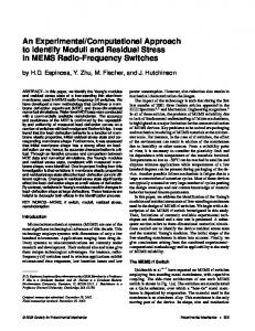
Figure 1.1. System layout of (a) a traditional imaging system and (b) a computational imaging system.

Aperture stop Detector array

Cubic phase mask Object

Y−axis

Reconstruction filter Intermediate image

Z−axis X−axis

Final image

Imaging optics

Figure 1.2. Extended depth of field imaging system layout (image examples are taken from Ref. [7]).

18 post-processing sub-system to form the image. The extended depth of field (EDOF) imaging system, described in Ref. [4], is an example of a computational imaging system. Fig. 1.2 shows the system layout of this EDOF imaging system. Note that it consists of a front-end optical system to form an intermediate image on the sensor array that is subsequently processed by an image reconstruction algorithm to yield the final focused image. The EDOF is achieved by modifying a traditional optical imaging system with the addition of a cubic-phase mask in the aperture stop. The resulting optical point spread function (PSF) has a larger support compared to a traditional PSF and therefore, the optical image formed on the sensor array appears to be blurred. However, as the optical PSF is invariant over an extended range of object distances, a simple reconstruction filter can be used in the post-processing step to form the final image that is focused throughout an extended object volume. This imaging system demonstrates the potential of the computational imaging paradigm to yield designs with novel capabilities, like EDOF, that simply could not be achieved by a traditional imaging system without significant performance trade-offs. Nevertheless, it is important to recognize that this EDOF imaging system does not fully exploit the capabilities of the computational imaging paradigm. The true potential of computational imaging can only be realized via a jointoptimization of the optical and the post-processing degrees of freedom. The joint design methodology yields a larger and richer design space for the designer. In order to understand this advantage let us examine the multi-dimensional design space depicted in Fig. 1.3, the optical design parameters are represented on the vertical axis and the post-processing design parameters are shown on the horizontal axis. Note that the traditional approach constrains the designer to a relatively small design subspace, outlined in brown and green. The region outlined in brown represents a design sub-space resulting from optimization of only optical parameters without any consideration to the degrees of freedom available in the post-processing domain. In the traditional design methodology, the optical design is followed by the optimization of

19

Global optima

Maxima Minima

Optical domain parameters

Joint design space

Post−processing design sub−space

Optical design sub−space

Post−processing domain parameters

Figure 1.3. A two-dimensional illustration of the joint optical and post-processing design space. post-processing parameters, represented by the sub-space in the green region. This approach does not guarantee an overall optimal system design and it usually leads to a sub-optimal system performance. In contrast, the joint-optimization design method combines the degrees of freedom available from the optical and the post-processing domains expanding the design space to a larger volume, represented by the red outlined region. This larger design space encompasses potential designs that offer benefits such as lower system cost, reduced complexity, improved yields and perhaps most importantly optimal/near-optimal system performance. Another key aspect of the joint design methodology is that it inherently supports a task-specific approach to imaging system design. To support this assertion let us consider an example of imaging system design for a classification task. The traditional design approach would involve: 1) design an optical imaging system to maximize the fidelity of the output image measurement and 2) design a classification algorithm that operates on the image measurement and minimizes the probability of misclassifica-

20 tion. Note that in this approach the optical imaging system and the classification algorithm are designed separately (and sequentially). Typically, a classification algorithm involves two steps: the feature extraction step and the classification step. In the feature extraction step, the original high-dimensional image measurement is transformed (compressed) into a low-dimensional data vector that is referred to as a feature vector. This dimensionality reduction step effectively lowers the computational complexity of the subsequent classification step. Acquiring a high-dimensional image measurement and subsequently reducing it to a low-dimensional feature clearly represents an inefficient data measurement process and a poor utilization of optical design resources. Thus, the traditional approach results in an imaging system design with sub-optimal performance for the classification task. Alternatively, a more logical approach would suggest an optical imaging system design that directly measures the optimal low-dimensional feature(s) for post-processing such that it maximizes the task performance, within the system constraints. This approach yields a computational imaging system design that offers two main advantages: a) a direct feature measurement yields a higher measurement signal to noise ratio (SNR) and b) the number of detectors required is significantly reduced. The high measurement SNR directly translates into improved system performance. This type of imaging system, referred to as a feature-specific imager (FSI) or a compressive imager, is an example of a computational imaging system [6]. This example clearly illustrates that the computational imaging paradigm supports and enables a task-specific approach to imaging system design.

1.3.

Main Contributions

The task-specific approach to computational imaging system design is an emerging area of research. Barrett et al. have conducted an extensive task-based analysis of imaging systems for detection and classification tasks in the area of medical imag-

21 ing [8, 9, 10]. Their focus has been primarily on the performance of ideal Bayesian observers and human observers. However, the application of the task-specific approach within a joint-optimization design framework is a relatively unexplored area. In this dissertation, we apply a task-specific approach to maximize the performance of a computational imaging system for a given task within a joint-optimization design framework. We consider two separate example tasks in this work: a reconstruction task and a classification task. In each case, the computational imaging system is optimized to maximize the task performance as measured by a task-specific metric. For example, the reconstruction task employs the traditional root mean square error (RMSE) and resolution metrics to quantify the quality of the reconstructed images. In the case of the classification task, false rejection ratio (FRR) and false alarm ratio (FAR) statistics are used as task-specific metrics to evaluate the overall system performance. In addition to the two design studies, a novel information theoretic taskspecific metric is also derived. A formal design framework based on this task-specific metric is developed and applied to the design of a compressive imaging system for the task of target detection. More specifically, the main contributions of this dissertation work are as follows: 1. The application of the optical PSF engineering method to optimize the imaging system performance for a specific task is considered. This task-specific method is first applied to a reconstruction task to overcome the distortions introduced by the detector under-sampling in the sensor array. Simulation results show nearly a 20% improvement in RMSE for the optimized imaging system design relative to the conventional imaging system. The optical PSF engineering method is also successfully applied to the design of an iris-recognition imaging system to minimize the impact of detector under-sampling on the overall performance. The optimized iris-recognition imaging system design achieves a 33% lower FRR compared to the conventional imaging system design.

22 2. Development a formal task-specific framework for computational imaging system design based on a novel information theoretic task-specific metric. This metric, known as task-specific information (TSI), quantifies the information content of an imaging system measurement relevant to a specific task. The TSI metric can also be used to derive an upper-bound on the performance of any post-processing algorithm for a specific task. Therefore, within the proposed design framework, the TSI metric can be used improve the upper-bound on imaging system performance thereby allowing the designer to optimize the imaging system for a particular task. The utility of the TSI metric is investigated for a variety of target detection and classification tasks. The application of the TSI-based design framework to extend the depth of field of an imager by optical PSF engineering is also considered. 3. The TSI-based design framework is used to design several compressive imaging systems for a target detection task. The resulting optimized imaging system designs shows a significant performance improvement over the un-optimized imaging designs.

1.4.

Dissertation Organization

The rest of the dissertation is organized as follows: • Chapter 2 presents the application of the optical PSF engineering method, within a multi-aperture imaging architecture, to overcome the distortions due to under-sampling in the detector array. The reconstruction task is considered in this study. RMSE and resolution are used as task-specific metrics during the imaging system optimization process. In the simulation study, the optimized imaging system designs show significant improvement, both in terms of RMSE and resolution metrics, compared to imaging system with a traditional

23 diffraction-limited PSF. The experimental results support the performance improvements predicted by the simulation study. • The task of iris-recognition, in the presence of detector under-sampling, is considered in Chapter 3. A multi-aperture imaging system in conjunction with optical PSF engineering is employed to optimize the overall performance of the imaging system. The task-specific design framework employs the FAR and FRR metrics to quantify the imaging system performance in this study. The simulation results show a substantial improvement in iris-recognition performance as a result of PSF optimization compared to the design that employs a traditional optical PSF. • As emphasized by the design studies described in Chapter 2 and Chapter 3, the performance metric plays a crucial role in the task-specific approach to imaging system design. In Chapter 4, the notion of task-specfic information is introduced as an objective metric for task-specfic design. TSI is an information theoretic metric that is derived using the recently discovered relationship between estimation theory and mutual-information. This metric is applied to a variety of detection and classification tasks to demonstrate its utility for task-specific performance evaluation. A brief analysis of a TSI-based optical PSF engineering approach for extending the depth of field of an imager is also presented in the context of a texture-classification task. • Chapter 5 presents a formal task-specific design framework that utilizes the TSI metric to optimize a compressive imaging system for a target detection task. The optimized imaging system designs deliver substantial performance improvement over the conventional design. The implementation issues regarding compressive imaging systems and the computational complexity associated with the TSI-based design framework are also discussed.

24 • Chapter 6 draws conclusions from the various aspects of the task-specifc approach investigated in this dissertation and provides direction for future work relevant to the further development of the joint-optimization design framework for computational imaging systems.

25

Chapter 2

Optical PSF Engineering: Object Reconstruction Task The optical PSF represents a degree of freedom that can be exploited to optimize an imaging system for a specific task. In a digital imaging system, the detector can limit the overall resolution when the optical PSF is smaller than the extent of the detector, leading to under-sampling or aliasing. In this chapter, we apply the optical PSF engineering method to improve the overall system resolution beyond the detector-limit and also increase the object reconstruction fidelity in such undersampled imaging systems.

2.1.

Introduction

In a traditional (i.e. film-based) design paradigm the optical PSF is typically viewed as the resolution-limiting element and therefore, optical designers strive for an impulselike PSF. Digital imagers however, employ photodetectors that are sometimes large relative to the extent of the optical PSF and in such cases the resulting pixel-blur and/or aliasing can become the dominant distortion limiting overall imager performance. This is illustrated by Fig. 2.1(a). This figure is a one-dimensional depiction of the image formed by a traditional camera when two point objects are separated by a sub-pixel distance. We see that the resulting impulse-like PSFs are imaged onto essentially the same pixel leading to spatial ambiguity and hence a loss of resolution. In such an imager the resolution is said to be pixel-limited [11]. The effect depicted in Fig. 2.1(a) may also be understood by noting that the detector array under-samples the image and therefore, introduces aliasing. The gen-

26 eralized sampling theorem by Papoulis [12] provides a mechanism through which this aliasing distortion can be mitigated. The theorem states that a bandlimited signal (−Ω ≤ ω ≤ Ω) can be completely/perfectly reconstructed from the sampled outputs of R non-redundant (i.e., diverse) linear channels, each of which employs a sample rate of

2Ω R

(i.e., each of the R signals is under-sampled at

1 R

the Nyquist rate). This theo-

rem suggests that the aliasing distortion can be reduced by combining multiple undersampled/low-resolution images to obtain a high-resolution image. A detailed description of this technique can be found in Borman [13]. This approach has been used by several researchers in the image processing community [11, 14, 15, 16, 17, 18] and was recently adopted for use in the TOMBO (Thin observing module with bounded optics) imaging architecture [19, 20]. The TOMBO system was designed to simultaneously acquire multiple low-resolution images of an object through multiple lenslets in an integrated aperture. The resulting collection of low-resolution measurements is then processed to yield a high-resolution image. Within the TOMBO system the multiple non-redundant images were obtained via a diverse set of sub-pixel shifts. The use of other forms of diversity including magnification, rotation, and defocus has also been considered [21]. However, it is important to note that these methods of obtaining measurement diversity do not fully exploit the optical degrees of freedom available to the designer. The approach described in this chapter will utilize PSF engineering in order to obtain additional diversity from a set of sub-pixel shifted measurements. The optical PSF of a digital imager may be viewed as a mechanism for encoding object information so as to better tolerate distortions introduced by the detector array. From this viewpoint an impulse-like optical PSF may be sub-optimal [22, 23]. To support this assertion let us consider the scenario depicted in Fig. 2.1(b), it shows an image of two point objects formed using a non-impulse-like PSF. The two point objects are displaced by the same amount as in Fig. 2.1(a). We see that the use of an extended PSF enables the extraction of sub-pixel position information from the sampled detector outputs. For example, a simple correlation-based processor [24] can

27

(a)

(b)

Figure 2.1. Schematic depicting the effect of pixel-limited resolution: (a) optical PSF is impulse-like and (b) engineered optical PSF is extended. yield the PSF centroid/point-source location to sub-pixel accuracy, given sufficient measurement signal-to-noise ratio (SNR). In this chapter, we study the performance of one such extended PSF design obtained by placing a pseudo-random phase mask in the aperture-stop of a conventional imager. Our choice of pseudo-random phase mask has been motivated in part by the pseudo-random sequences found in CDMA multi-user communication systems [25, 26] and in part by a study in Ref. [27] which found pseudo-random phase masks to be efficient in an information-theoretic sense for imaging sparse volumetric scenes. In the context of multi-user communications, pseudo-random sequences are used to encode the information of each end-user. These encoded messages are combined and transmitted over a common channel. The structure of the encoding is then used at the receiver side to extract individual messages from the super-position. In a digital imaging system, the optical PSF serves a similar purpose in terms of encoding the location of individual resolution elements that comprise the object. The pixels within a semiconductor detector array measure a super-position of responses from each resolution element in the object. Further the spatial integration across the finite pixel size of the detector array leads to spatial blurring. These signal transformations imposed by the detector array must be inverted via decoding. In the next section, we describe the mathematical model of the imaging system and the pseudo-random phase mask used to engineer the extended

28 optical PSF.

2.2.

Imaging System Model

Consider a linear model of a digital imaging system. Mathematically, we can represent the system as g = Hcd fc + n,

(2.1)

where fc is the continuous object, g is the detector-array measurement vector, Hcd is the continuous-to-discrete imaging operator and n is additive measurement noise vector. For simulation purposes we use a discrete representation f of the continuous object fc . This discrete representation f can be obtained from fc as follows [28] Z fi = fc (~r)φi (~r)dr 2 , (2.2) S∩Φi

where S is the object support, {φi } is an analysis basis set, Φi is the support of

ith basis function φi and fi is the ith element of the object vector f. Note that we obtain an approximation fa of the original continuous object fc from its discrete representation f as follows [28] fa (~r) =

N X i=1

fi · ψi (~r),

(2.3)

where N is the dimension of the discrete object vector and {ψi } is a synthesis basis set which can be chosen to be the same as the analysis basis set {φi }. Here we use the pixel function to construct our analysis and synthesis basis sets. The pixel function is defined as

and

r − iΩ 1 r φi (r) = rect Ωr Ωr Z φi(r)φj (r)dr 2 = δij ,

(2.4)

Φi ∩Φj

where 2Ωr is the size of the resolution element in the continuous object that can be accurately represented by this choice of basis set. Note that the pixel functions

29 {φi } form an orthonormal basis. We set the object resolution element size equal to the diffraction-limited optical resolution of the imager to ensure that the discrete representation of the object does not incur any loss of spatial resolution. Here we adopt the Rayleigh’s criteria [29] to define resolution. Henceforth, all references to resolution will represent the Rayleigh resolution. The imaging equation is modified to include the discrete object representation as follows g = Hf + n,

(2.5)

where H is the equivalent discrete-to-discrete imaging operator: H is therefore a matrix. The imaging operator H includes the optical PSF, the detector PSF, and the detector sampling. The vectors f, g, and n are lexicographically arranged onedimensional representations of the two-dimensional object, image, and noise arrays, respectively. Consider a diffraction-limited PSF of the form: h(r) = sinc2

r R

, with Rayleigh

resolution R. The Nyquist sampling theorem requires the detector spacing to be at most

R . 2

When this requirement is met, the imaging operator H has full rank

(condition-number → 1) allowing a reconstruction of the object up to the optical resolution. However, when the optical PSF has an extent (2R) that is smaller than the detector spacing, the image measurement is aliased and the imaging operator H becomes singular (condition-number → ∞). Under these conditions the object cannot be reconstructed up to the optical resolution. Also note that due to under-sampling the imaging operator H is no longer shift-invariant but only block-wise shift-invariant even if the imaging optics itself is shift-invariant. As mentioned in the previous section, one method to overcome the resolution constraint imposed by the pixel-size is to use multiple sub-pixel shifted image measurements. The sub-pixel shift δ may be obtained either by a shift in the imager position or through object movement. The ith sub-pixel shifted image measurement

30 Apertute stop Pseudo−random phase mask

Detector−array

Object

Z−axis

Y−axis

Lens system

X−axis

Figure 2.2. Imaging system setup used in the simulation study. gi with shift δi can be represented as gi = Hi f + ni ,

(2.6)

where Hi represents the imaging operator associated with the sub-pixel shift δi . For a set of K such measurements we can write the composite image measure ment by concatenating the individual vectors as, g = g1 g2 · · · gK and similarly n = n1 n2 · · · nK . The overall multi-frame composite imaging system can be expressed as

g = Hc f + n,

(2.7)

where Hc is the composite imaging operator. By combining several sub-pixel shifted image measurements, the condition number of the composite imaging operator Hc can be progressively improved and the overall resolution can be increased towards the optical resolution limit. Ideally, the sub-pixel shifts should be chosen in multiples of

D K

so as to minimize the condition-number of the forward imaging operator Hc ,

where D is the detector spacing [30]. We are interested in designing an extended optical PSF for use within the sub-pixel shifting framework. The use of an extended optical PSF can improve the conditionnumber of the imaging operator Hc . We consider an extended optical PSF obtained by placing a pseudo-random phase mask in the aperture-stop of a conventional imager, as shown in Fig. 2.2. For simulation purposes the aperture-stop is defined on a discrete spatial grid. Therefore, the pseudo-random phase mask is represented by an array,

31 −3

14

−3

x10

x 10 1.6

12

1.4 10

Amplitude

Amplitude

1.2 8

6

1 0.8 0.6

4 0.4 2

0

0.2

−15

−10

−5 0 5 Spatial dimension [µm]

10

15

0

−15

−10

(a)


10

15

(b)

Figure 2.3. Example simulated PSFs: (a) Conventional sinc2 (·) PSF and (b) PSF obtained from PRPEL imager. each element of which corresponds to the phase at given a position on the discrete spatial grid. The pseudo-random phase mask is synthesized in two steps: (1) generate a set of identical independently distributed random numbers distributed uniformly on the interval [0, ∆] to populate the phase array and (2) convolve this phase array with a Gaussian filter kernel which is a Gaussian function with standard-deviation ρ, sampled on the discrete spatial grid. The resulting set of random numbers define the phase distribution Φ(r) of the pseudo-random phase mask. The phase mask is thus a realization of a spatial Gaussian random process which is parameterized by its roughness ∆ and correlation length ρ. The auto-correlation function of this phase distribution is given by

∆2 r2 RΦΦ (r) = exp − 2 . 12 4ρ

(2.8)

The incoherent PSF is related to the phase-mask profile Φ(r) as follows [28] 2 r Ac , (2.9) Tpupil − psf (r) = (λf )4 λf Tpupil (ω) = F {exp[j2π(nr − 1)Φ(r)/λ]tap (r)} , (2.10) where Ac is normalization constant with units of area, nr is the refractive index of the lens, f is the back focal length, tap (r) is the aperture function and F denotes the forward Fourier transform operator.

32 Fig. 2.3(a) shows a simulated impulse-like PSF and Fig. 2.3(b) an extended PSF resulting from simulating a pseudo-random phase mask with parameters ∆ = 1.5λc and ρ = 10λc , where λc is the operating center wavelength. Here we set λc =550 nm and the imager F/# = 1.8. Assuming a detector size of 7.5 µm, the support of extended PSF extends over roughly six detectors, in contrast with a sub-pixel extent of 2 µm for the impulse-like PSF. The extended PSF will therefore accomplish the desired encoding; however, it will do so at the cost of measurement SNR. Because the extended PSF is spread over several pixels, its photon count per detector is lower than that for the impulse-like PSF for a point-like object. Assuming a constant detector noise, the measurement SNR per detector for the extended PSF is thus lower than that of the impulse-like PSF. For more general objects, the extended PSF results in a reduced contrast image with a commensurate SNR reduction, though smaller than for point-like objects. In the next section, we present a simulation study to quantify the tradeoff between the overall imaging resolution and the SNR for two candidate imagers that use multiple sub-pixel shifted measurements: (a) the conventional imager and (b) the pseudo-random phase enhanced lens (PRPEL) imager.

2.3.

Simulation results

For the purposes of the simulation study, we consider only one-dimensional objects and image measurements. The target imaging system has a modest specification with an angular resolution of 0.2 mrad and an angular field of view(FOV) of 0.1 rad. The conventional imager uses a lens of F/# = 1.8 and back focal length 5 mm. We assume that the lens is diffraction-limited and the optical PSF is shift-invariant. The detector array in the image plane has a pixel size of 7.5 µm with a full-well capacity (FWC) of 45000 electrons and a 100% fill factor. We further assume that the imager’s spectral bandwidth is limited to 10 nm centered at λc =550 nm. For the PRPEL imager the only modification is that the lens is followed by a pseudo-random phase mask with

33 parameters ∆ and ρ. We assume a shot-noise limited SNR=46 dB (20 log10

√

F W C) given by the FWC

of the detector element. The shot-noise is modeled as equivalent AWGN with variance σ 2 = F W C. The under-sampling factor for this imager is F = 15. This implies that for an object vector f of size N ×1 the resulting image measurement vector gi is of size M × 1 where M =

N . F

For the target imager, these values are N = 512 and M = 34.

Note that the block-wise shift-invariant imaging operator Hc is of size KM × N. To improve the overall imager performance we consider multiple sub-pixel shifted image measurements or frames. These frames result from moving the imager with respect to the object by a sub-pixel distance δi . Here it is important to constrain the number of photons per frame to ensure a fair comparison among imagers using multiple frames. We have two options: (a) assume that each imager has access to the same finite number of photons and (b) assume that each frame of each imager has access to the same finite number of photons. Option (b) may be physical under certain conditions; however, the results that are obtained will be unable to distinguish between improvements arising from frame diversity versus improvements arising from increased SNR. We therefore utilize option (a) because it is the only option that allows us to study how best to use fixed photon resources. As a result, the photon count for each frame is normalized to

F K

in this simulation study.

The inversion of the composite imaging Eq. (2.7), is based on the optimal linearminimum-mean-squared-error (LMMSE) operator W. The resulting object estimate is given by bf = Wg,

(2.11)

T −1 W = Rf HT c (Hc Rf Hc + Rn ) .

(2.12)

where W is defined as [31]

Rf is the auto-correlation matrix for the object vector f and Rn is the auto-correlation matrix of the noise vector n. Because the composite imaging operator Hc is not shift-

34

0 Burg estimate Power law η=1.0 Power law η=1.4 Power law η=2.0

Log power spectral density

−10 −20 −30 −40 −50 −60 −70 −80 20

(a)

40

60 80 100 120 Angular frequency [cycles/degree]

140

160

(b)

Figure 2.4. Reconstruction incorporates object priors: (a) object class used for training and (b) power spectral density obtained from the object class and the best powerlaw fit used to define the LMMSE operator. invariant the LMMSE solution does not reduce to the well-known Wiener filter. The noise auto-correlation matrix reduces to a diagonal matrix under the assumption of independent and identically distributed (i.i.d.) noise and therefore, can be written as Rn = σ 2 I. The object auto-correlation matrix Rf incorporates object prior knowledge within the reconstruction process as a regularizing term. Here we obtain the object auto-correlation matrix from a power-law power spectral density (PSD):

1 , fη

that serves as a good model for natural images [32, 33, 34]. A power-law PSD was computed to model the class of 10 objects shown in Fig. 2.4(a) chosen to represent a wide variety of scenes (rows and columns of these scenes are used as 1D objects). Fig. 2.4(b) shows several power law PSDs plotted along with the PSD obtained using Burg’s method [35] on 3 objects chosen from the set in Fig. 2.4(a). The power-law PSD(η = 1.4) is used to model the PSD of the object class as it is applicable to wider range of natural images compared to PSD models such as Burg’s that are obtained for a specific set of objects. The value of power-law PSD parameter η was obtained by a least-squares fit to the Burg’s PSD estimate. In order to quantify the performance of both the PRPEL and the conventional

35

1 Post−processed PSF 2 Fitted sinc (.) PSF

0.9 0.8 0.7

Amplitude

0.6 0.5 0.4 0.3

Estimated resolution=0.4mrad

0.2 0.1 0 −2

−1

0

1

2

Angular dimension [mrad]

Figure 2.5. Rayleigh resolution estimation for multi-frame imagers using a sinc2 (·) fit to the post-processed PSF. imaging systems we employ two metrics: (a) Rayleigh resolution and (b) normalized root-mean-square-error (RMSE). The Rayleigh resolution of a composite multi-frame imager is found by using a point-source object and applying the LMMSE operator to the K image frames. The resulting point-source reconstruction represents the overall PSF of the computational imager. A least-squares fit of a diffraction-limited sinc2 (·) PSF to the overall imager PSF is used to obtain the resolution estimate. Fig. 2.5 illustrates this resolution estimation method with an example of a post-processed PSF and the associated sinc2 (·) fit. The second imager performance metric uses RMSE to quantify the quality of a reconstructed object. The RMSE metric is defined as, q h||b f − f||2 i × 100%, (2.13) RMSE = 255 where 255 is the peak object pixel value. Here, the expectation h·i is taken over both the object and the noise ensembles. We have used all columns and rows of the 2D objects shown in Fig. 2.4(a) to form a set of 1D objects for computing the RMSE metric in the simulation study. First, we consider the conventional imager. The sub-pixel shift for each frame is chosen randomly. The performance metrics are computed and averaged over 30

36

1.6 7

Angular resolution [mrad]

RMSE [% of dynamic range]

1.4 6

5

4

3

1.2 1 0.8 0.6 0.4

2 0.2 1

2

3

4

5

6

7 8 9 10 11 Number of frames − K

(a)

12

13

14

15

16

1

Diffraction−limited resolution 2

3

4

5

6

7

8

9

10

11

12

13

14

15

16

Number of frames − K

(b)

Figure 2.6. Conventional imager performance with number of frames (a) RMSE and (b) Rayleigh resolution. sub-pixel shift-sets for each value of K. Fig. 2.6(a) shows a plot of the RMSE versus the number of frames K. We observe that the RMSE decreases with the number of frames, as expected. This result demonstrates that additional object information is accumulated through the use of diverse (i.e., shifted) channels: as the number of frames increases, the condition-number of the composite imaging operator Hc improves. The reason that the RMSE does not converge to zero for K = 16 is because the detector noise ultimately limits the minimum reconstruction error. The resolution of the overall imager is plotted against the number of frames K in Fig. 2.6(b). Observe that the resolution improves with increasing K, converging towards the optical resolution limit of 0.2 mrad. The resolution obtained with K = 16 is not equal to the diffraction-limit because this data represents an average resolution over a set of random sub-pixel shift-sets. When the sub-pixel shifts are chosen as multiples of

D F

the resolution achieved for K = 16 is indeed equal to the optical resolution limit. The PRPEL imager employs a pseudo-random phase mask to modify the impulselike optical PSF. The phase mask parameters ∆ and ρ jointly determine the statistics of the spatial intensity distribution and the extent of the optical PSF. We design an optimal phase mask by setting ρ to a constant(10λc ) and finding the value of ∆ that

37

0.7

5

4.8

0.6



0.65

0.55 0.5 0.45 0.4

4.6

4.4

4.2

4

0.35 3.8 1

2

3 4 5 6 Mask roughness − ∆ [λ], ρ=10λ

7

8

9

0.5

1

1.5

2 2.5 3 3.5 4 4.5 Mask roughness − ∆[λ] ρ=10[λ]

5

5.5

6

Figure 2.7. PRPEL imager performance versus mask roughness parameter ∆ with ρ = 10λc and K = 3: (a) Rayleigh resolution and (b) RMSE. maximizes the imager performance for a given K. Fig. 2.7(a) presents representative data quantifying imager resolution as a function of ∆ with ρ = 10λc and K = 3. This plot shows the fundamental tradeoff between the condition number of the imaging operator and the SNR cost. Note that for small values of ∆ the PSF is impulse-like. As the value of ∆ increases the PSF becomes more diffuse as shown in Fig. 2.3(b). This results in an improvement in condition number; however, as the PSF becomes more diffuse the photon-count per detector decreases resulting in an overall decrease in measurement SNR. Fig. 2.7(a) shows that optimal resolution is achieved for ∆ = 7λc . Fig. 2.7(b) demonstrates a similar trend in RMSE versus ∆ with ρ = 10λc and K = 3. The optimal value of ∆ under the RMSE metric is ∆ = 1.5λc . Note that the optimal values of ∆ are different for the resolution and RMSE metrics. The resolution of an imager is determined by its spatial frequency response alone; whereas, the RMSE is dependent on the spatial frequency response as well as the object statistics. Therefore, the value of ∆ that maximizes the resolution metric may result in an imager with a particular spatial frequency response that may not achieve the minimum RMSE given the object statistics and detector noise. All the subsequent results for the PRPEL imager are obtained for the optimal value of ∆ which will therefore be a function of

38

8 Lens imager PRPEL imager

1.6

Lens imager PRPEL imager 7



1.4 1.2 1 0.8 0.6 0.4 0.2

6

5

4

3

2 Diffraction−limited resolution

1

2

3

4

5

6

7

8

9

10

11

12

13

14

15

16


1 1

2

3

4

5

6 7 8 9 10 11 Number of Frames − K

12

13

14

15

16

Figure 2.8. PRPEL and conventional imager performance versus number of frames: (a) Rayleigh resolution, and (b) RMSE. K, σ and the metric (RMSE or resolution). Fig. 2.8(a) presents the resolution performance of both the PRPEL and the conventional imagers as a function of the number of frames K. We note that the PRPEL imager converges faster than the conventional imager. A resolution of 0.3 mrad is achieved with only K = 4 by the PRPEL imager in contrast with K = 12 for the conventional imager. A plot comparing the RMSE performance of the two imagers is shown in Fig. 2.8(b). We note that the PRPEL imager is consistently superior to the conventional imager. For K = 4 the PRPEL imager achieves an RMSE of 3.5% as compared with RMSE of 4.3% for the conventional imager.

2.4.

Experimental results

An experimental demonstration of the PRPEL imager was undertaken in order to validate the performance improvements predicted by simulation. Fig. 2.9 shows the experimental setup along with the relevant physical dimensions. A Santa Barbara Instrument Group ST2000XM CCD was used as the detector array. The CCD consists of a 1600 × 1200 detector array, with a detector size of 7.4 µm, 100% fill factor and a FWC of 45000 electrons. The detector output from the CCD is quantized with a

Fujinon Lens 16mm

FOV

Y−axis

210µm

210µm Zoom lens(2.5x) Diffuser(phase mask)

Aperture = 20mm

SBIG CCD array 7.4µm

39

Fiber−tip X−axis 540mm

Figure 2.9. Schematic of the optical setup used for experimental validation of the PRPEL imager. 16 bit analog-digital convertor yielding a dynamic range of [0 − 64000] digital counts. During the experiment the CCD is cooled to −10◦ C, to minimize electronic noise.

The experimental setup uses a Fujinon’s CF16HA-1 TV lens operated at F/#=4.0. A circular holographic diffuser from Physical Optical Corporation is used as a pseudorandom phase mask. The divergence angle(full-width half-maximum) of the diffuser is 0.1◦ . A zoom lens with magnification 2.5x is used to decrease the divergence angle of the diffuser. The actual phase statistics of the diffuser are not disclosed by the manufacturer. Therefore, to relate the physical diffuser to the pseudo-random phase mask model we compute phase mask parameters ∆ and ρ that yield a PSF similar to the one produced by the physical diffuser. The phase mask parameters ∆ = 2.0λc and ρ = 175λc yield the PSF shown in Fig. 2.10(c). Comparing this PSF to the PRPEL experimental PSF shown in Fig. 2.10(b), we note that they are similar in appearance. This comparison although qualitative suggests that the physical diffuser might possess statistics similar to the pseudo-random phase mask model described here. The Rayleigh resolution of the conventional optical PSF was estimated to be 5 µm or 0.31 mrad. This yields an under-sampling factor of F = 3 along each direction. This implies that a total of F 2 = 9 frames are required to achieve the full optical

40

−3

−2

−2

−1

−1

−1

0

[mrad]

−3

−2

[mrad]

[mrad]

−3

0

0

1

1

1

2

2

2

3

3 −3

−2

−1

0

1

2

3

3 −3

−2

−1

[mrad]

[mrad]

(a)

0

(b)

1

2

3

−3

−2

−1

0

1

2

3

[mrad]

(c)

Figure 2.10. Experimentally measured PSFs obtained from the (a) conventional imager, (b) PRPEL imager, and (c) simulated PRPEL PSF with phase mask parameters ∆ = 2.0λc and ρ = 175λc. resolution. The FOV for the experiment is 10 mrad×10 mrad consisting of 64 × 64 pixels each of size 0.156 mrad×0.156 mrad. The highly under-sampled nature of the conventional imager as well as the extended nature of the PRPEL PSF demand careful system calibration. Our calibration apparatus consisted of a fiber-tip pointsource mounted on a X-Y translation stage that can be scanned across the object FOV. The 50 µm fiber core diameter in object space yields a 0.6 µm diameter point in image space(system magnification=

1 84

x)which is much smaller than the detector

size of 7.4 µm. Therefore, we can assume that the fiber-tip serves a good point-source approximation for imager calibration purpose. Also note that the exiting radiation from the fiber-tip(numerical aperture=0.22) overfills the entrance aperture of the imager optics by a factor of 12. The motorized translation stage is controlled by a Newport EPS300 motion controller. The fiber tip is illuminated by a white lightsource filtered by a 10 nm bandpass filter centered at λc =535 nm. The calibration procedure involves scanning the fiber-tip over each object pixel position in the FOV and for each such position, recording the discrete PSF at the CCD. To obtain reliable PSF data during calibration we average 32 CCD frames to increase the measurement SNR. To obtain PSF data with a particular sub-pixel shift, the calibration process is repeated after shifting the FOV by that sub-pixel amount. This calibration data is

41


0.55

Lens imager PRPEL imager

0.5

0.45

0.4

0.35 Optical resolution 0.3 1

2

3

4

5

6

7

8

9


Figure 2.11. Experimentally measured Rayleigh resolution versus number of frames for both the PRPEL and conventional imagers. subsequently used to construct the composite imaging operator Hc and compute the LMMSE operator W using Eq. (2.12). The same calibration procedure is used for both the conventional and the PRPEL imagers. The experimental PSFs for these two imagers are shown in Fig. 2.10(a) and Fig. 2.10(b). The PSF of the conventional imager is seen to be impulse-like; whereas, the PSF of the PRPEL imager has a diffused/extended shape as expected. The resolution estimation procedure described in the previous section is once again employed to estimate the resolution of the two experimental imagers. Fig. 2.11 presents the plot of resolution versus number of frames K from the experiment data. Three data points are obtained at K = 1, 4, and 9. The sub-pixel shifts (in microns) used for these measurements were: (0,0) for K=1, (0,0), (0,3.7), (3.7,0), (3.7,3.7) for K=4, and (0,0), (0,2.5), (0,5), (2.5,0), (2.5,2.5), (2.5,5), (5,0), (5,2.5), (5,5) for K = 9. Note the imager resolution is estimated using test data that is distinct from the calibration data. As predicted in simulation, we see that the PRPEL imager outperforms the conventional imager at all values of K. We observe that the PRPEL resolution nearly saturates by K = 4. A maximum resolution gain of 13% is achieved at K = 4 by the PRPEL imager relative to conventional imager. Note that even at K = 9 the

−5

−5

−4

−4

−3

−3

−2

−2

−1

−1 [mrad]

[mrad]

42

0

0

1

1

2

2

3

3

4

4

5 −5

−4

−3

−2

−1

0 [mrad]

(a)

1

2

3

4

5

5 −5

−4

−3

−2

−1

0

1

2

3

4

5

[mrad]

(b)

Figure 2.12. The USAF resolution target (a) Group 0 element 1 and (b) Group 0 elements 2 and 3. resolution achieved by both the imagers is slightly poorer than the estimated optical resolution of 0.31 mrad. This can be attributed to errors in the calibration process, which include non-zero noise in the PSF measurements and shift errors due to the finite positioning accuracy of the computer-controlled translation stages. A USAF resolution target was used to compare the object reconstruction quality of the two imagers. Because the imager FOV is relatively small (10 mrad×10 mrad/ 13.44 mm×13.44 mm) we used two small areas of the USAF resolution target shown in Fig. 2.12(a) and Fig. 2.12(b). In Fig. 2.12(a) the spacing between lines of group 0 element 1 is 500 µm in object space or equivalently 0.37 mrad. Similarly in Fig. 2.12(b) the line spacings for group 0 elements 2 and 3 are 0.33 mrad and 0.30 mrad respectively. Given the optical resolution of the experimental system, we expect that group 0 element 3 should be resolvable by both the conventional and PRPEL imagers. Fig. 2.13 presents the raw detector measurements of USAF group 0 element 1 from the two imagers. Consistent with the measured degree of under-sampling, the imagers are unable to resolve the constituent line elements in the raw data. Fig. 2.14 shows reconstructions from the two multi-frame imagers for the same object using K = 1, 4, and 9 sub-pixel shifted frames. We observe that for K = 1 neither imager can resolve the object. For K = 4 however, the PRPEL imager clearly resolves the

43

−5

−5

−4

−4 −3

−2

−2

−1

−1 [mrad]

[mrad]

−3

0

0

1

1

2

2

3

3

4 5 −5

4 −4

−3

−2

−1

0 [mrad]

(a)

1

2

3

4

5

5 −5

−4

−3

−2

−1

0 1 [mrad]

2

3

4

5

(b)

Figure 2.13. Raw detector measurements obtained using USAF Group 0 element 1 from (a) the conventional imager and (b) the PRPEL imager. lines in the object; whereas, the conventional imager does not resolve them clearly. Fig. 2.15(a) shows a horizontal line scan through the object and LMMSE reconstructions for K = 4, affirming our observation that the PRPEL imager achieves superior contrast to that of the conventional imager. For K = 9 we note that both imagers resolve the object equally well. Next we consider USAF group 0 elements 2 and 3 object whose reconstructions are shown in Fig. 2.16. As before, for K = 1 neither imager can resolve the object. However, for K = 4 the PRPEL imager clearly resolves element 2 and barely resolves element 3. In contrast, the conventional imager barely resolves element 2 only. This is also evident in the horizontal line scan of the object and the LMMSE reconstructions shown in Fig. 2.15(b). Both imagers achieve comparable performance for K = 9, completely resolving the object. We observe that despite having precise channel knowledge we obtain poor reconstruction results for the case K = 1. This points to the limitations of linear reconstruction techniques that can not include powerful object constraints such as positivity and finite support. However, non-linear reconstruction techniques such as iterative back projection(IBP) [36] and maximum-likelihood expectation-maximization(MLEM) [37] can easily incorporate these constraints. The Richardson-Lucy(RL) algorithm [38, 39] based on the MLEM principle has been shown to be one such effective reconstruction

−4

−4

−3

−3

−2

−2

−1

−1 [mrad]

[mrad]

44

0

0

1

1

2

2

3

3

4

4 −4

−3

−2

−1

0

1

2

3

4

−4

−3

−2

−1

−4

−4

−3

−3

−2

−2

−1

−1

0

1

2

2

3

3

4

4 −3

−2

−1

0

1

2

3

4

−4

−3

−2

−1

−4

−4

−3

−3

−2

−2

−1

−1

0

1

2

2

3

3

4

4 −2

−1

0 [mrad]

3

4

0

1

2

3

4

1

2

3

4

0

1

−3

2

[mrad]

[mrad]

[mrad]

[mrad]

−4

1

0

1

−4

0 [mrad]

[mrad]

[mrad]

[mrad]

1

2

3

4

−4

−3

−2

−1

0 [mrad]

Figure 2.14. LMMSE reconstructions of USAF group 0 element 1 with left column for PRPEL imager and right column for conventional imager: top row for K=1, middle row for K=4, and bottom row for K=9.

45

Object PRPEL reconstruction Lens reconstruction 1

0.8

0.6

0.4

0.2

0 −5

−4

−3

−2

−1

0

1

2

3

4

5

1

2

3

4

5

[mrad]

(a)

Object PRPEL reconstruction Lens reconstruction 1 0.8 0.6 0.4 0.2 0 −5

−4

−3

−2

−1

0 [mrad]

(b)

Figure 2.15. Horizontal line scans through the USAF target and its LMMSE reconstruction for conventional and PRPEL imagers for K=4: (a) group 0 elements 1 and (b) group 0 elements 2 and 3.

46

−4 −4

−3

−3 −2 −2 −1 [mrad]

[mrad]

−1 0

0 1

1

2 2 3 3 4 −4

4 −3

−2

−1

0

1

2

3

4

−4

−3

−2

−1

−4

−3

−3

−2

−2

−1

−1 [mrad]

[mrad]

−4

0

1

2

2

3

3

4

4 −3

−2

−1

0

1

2

3

4

−4

−3

−2

−1

−4

−4

−3

−3

−2

−2

−1

−1

0

1

2

2

3

3

4

4 −2

−1

0 [mrad]

3

4

0

1

2

3

4

1

2

3

4

0

1

−3

2

[mrad]

[mrad]

[mrad]

[mrad]

−4

1

0

1

−4

0 [mrad]

[mrad]

1

2

3

4

−4

−3

−2

−1

0 [mrad]

Figure 2.16. LMMSE reconstructions of USAF group 0 element 2 and 3 with left column for PRPEL imager and right column for conventional imager: top row for K=1, middle row for K=4, and bottom row for K=9.

47 technique. The RL algorithm is a multiplicative iterative scheme where the k + 1th object update denoted by ˆf (k+1) is defined as [28], KM gm 1 X fˆn(k+1) = fˆn(k) Hcmn , sn m=1 Hcˆf (k) m

sn =

KM X

(2.14)

Hcmn ,

m=1

where the subscript denotes the corresponding element of a vector or a matrix. Note that if all elements of the composite imaging matrix Hc , the raw image measurement g and the initial object estimate ˆf (0) are positive then all subsequent estimates of the object are guaranteed to be positive, thereby achieving the positivity constraint. Further, by setting the appropriate elements of ˆf (0) to 0 we can implement the finite support constraint in the RL algorithm. We apply the RL algorithm described above to the experimental data in an effort to improve reconstruction quality, especially for K = 1. A constant positive vector is used as an initial object estimate i.e. ˆf (0) = c where ci = a > 0, ∀i. Fig. 2.17 and Fig. 2.18 shows the RL object reconstructions of the USAF group 0 element 1 and USAF group 0 elements 2 and 3 respectively. As expected, the RL algorithm yields a substantial improvement in reconstruction quality over the LMMSE processor. This improvement is most notable for the K = 1 case. In Fig. 2.17 we observe that the PRPEL imager delivers better results compared to the conventional imager for K = 1 and K = 4. The horizontal line scans in Fig. 2.19(a) show that the PRPEL imager maintains a superior contrast compared to the conventional imager for K = 4. From Fig. 2.18 we observe that for K = 1 the PRPEL imager begins to resolve element 2 whereas the conventional imager still fails to resolve element 2. For K = 4, element 2 is clearly resolved and element 3 is just resolved by the PRPEL imager. In comparison the conventional imager barely resolves element 2. These observations are confirmed by the horizontal line scan plots shown in Fig. 2.19(b). Overall the experimental reconstruction and resolution results confirm the conclu-

−4

−4

−3

−3

−2

−2

−1

−1 [mrad]

[mrad]

48

0

0

1

1

2

2

3

3

4

4 −4

−3

−2

−1

0

1

2

3

4

−4

−3

−2

−1

−4

−3

−3

−2

−2

−1

−1 [mrad]

[mrad]

−4

0

1

2

3

4

1

2

3

4

1

2

3

4

0

1

1

2

2

3

3

4

4 −4

−3

−2

−1

0

1

2

3

4

−4

−3

−2

−1

−4

−3

−3

−2

−2

−1

−1 [mrad]

−4

0

0

1

1

2

2

3

3

4

4 −4

−3

−2

−1

0 [mrad]

0 [mrad]

[mrad]

[mrad]

0 [mrad]

[mrad]

1

2

3

4

−4

−3

−2

−1

0 [mrad]

Figure 2.17. Richardson-Lucy reconstructions of USAF group 0 element 1 with left column for PRPEL imager and right column for conventional imager: top row for K=1, middle row for K=4, and bottom row for K=9.

−4

−4

−3

−3

−2

−2

−1

−1 [mrad]

[mrad]

49

0

0

1

1

2

2

3

3

4

4 −4

−3

−2

−1

0

1

2

3

4

−4

−3

−2

−1

−4

−4

−3

−3

−2

−2

−1

−1

0

1

2

3

4

1

2

3

4

1

2

3

4

0

1

1

2

2

3

3 4

4 −4

−3

−2

−1

0

1

2

3

4

−4

−3

−2

−1

−4

−3

−3

−2

−2

−1

−1 [mrad]

−4

0

0

1

1

2

2

3

3

4

4 −4

−3

−2

−1

0 [mrad]

0 [mrad]

[mrad]

[mrad]

0 [mrad]

[mrad]

[mrad]

[mrad]

1

2

3

4

−4

−3

−2

−1

0 [mrad]

Figure 2.18. Richardson-Lucy reconstructions of USAF group 0 element 2 and 3 with left column for PRPEL imager and right column for conventional imager: top row for K=1, middle row for K=4, and bottom row for K=9.

50


−4

−3

−2

−1

0

1

2

3

4

5

1

2

3

4

5

[mrad]

(a)


−4

−3

−2

−1

0 [mrad]

(b)

Figure 2.19. Horizontal line scans through the USAF target and its Richardson-Lucy reconstruction for conventional and PRPEL imagers for K=4: (a) group 0 elements 1 and (b)group 0 elements 2 and 3. sions drawn from our simulation study; the PRPEL imager offers superior resolution and reconstruction performance compared to the conventional multi-frame imager.

2.5.

Imager parameters

The results reported here have demonstrated the utility of the PRPEL imager. In order to motivate a more general applicability of the PRPEL approach, there are two important parameters that require further investigation: pixel size and spectral-

51

5.5 Lens Imager PRPEL Imager

Lens Imager PRPEL Imager

5 RMSE [% of dynamic range]


0.7

0.6

0.5

0.4

0.3

4.5 4 3.5 3 2.5 2 1.5

0.2 1

Diffraction−limited resolution 2

3

1 4

5


(a)

6

7

8

1

2

3

4

5

6

7

8


(b)

Figure 2.20. (a) Rayleigh resolution and (b) RMSE versus number of frames for multi-frame imagers that employ smaller pixels and lower measurement SNR. bandwidth. We consider two case studies in which these imaging system parameters are modified in order to study their impact on overall imager performance. 2.5.1. Pixel size Here we consider the effect of smaller pixel size which is typical of CMOS detectors arrays, now commonly employed in many imagers. Consider a sensor having a pixel size of 3.2 µm resulting in a less severe under-sampling as compared with the 7.5 µm pixel size assumed earlier. This detector has a 100% fill-factor and a smaller FWC of 28000 electrons(lower SNR). All other parameters of the imaging system remain unchanged. The under-sampling factor for the new sensor is F = 7 and the photon-limited SNR is now 22dB. We repeat the simulation study of the overall imaging system performance for both the conventional imager and the PRPEL imager. Fig. 2.20(a) shows the plot of the resolution versus the number of frames for both imaging systems. This plot shows that for K = 2 the PRPEL imager achieves a resolution of 0.3 mrad while the conventional imager resolution is only 0.5 mrad. Fig. 2.20(b) shows the RMSE performance of the two imagers versus the number of frames. For K = 2 the PRPEL

52

−3

x 10

PSF − 10nm PSF − 150nm

1.6 1.4

Amplitude

1.2 1 0.8 0.6 0.4 0.2 0

−15

−10


10

15

Figure 2.21. The optical PSF obtained using PRPEL with both narrowband (10 nm) and broadband (150 nm) illumination. imager achieves a RMSE of 3.2% compared to 4.0% for the conventional imager, an improvement of nearly 20%. From these results we conclude that the PRPEL imager remains a useful option for imagers with CMOS sensors that have smaller pixels and a lower SNR. 2.5.2. Broadband operation Recall that all our simulation studies have assumed a 10 nm spectral bandwidth so far. In this section, we will relax this constraint and allow the spectral bandwidth to increase to 150 nm, roughly equal to the bandwidth of the green band of the visible spectrum. All other imaging system parameters remain unchanged (using the original 7.5 µm sensor). There is a two-fold implication of the increased bandwidth. First, because we accept a wider bandwidth, the photon count increases resulting in an improved measurement SNR. Within the PRPEL imager however, this SNR increase is accompanied by increased chromatic dispersion and a smoothing of the PRPEL PSF. This smoothing results in a worsening of the condition number for the PRPEL imager. To illustrate the dispersion effect, Fig. 2.21 shows a plot of the extended PRPEL PSF for both the 10 nm and the 150 nm bandwidths. The

53

8 Lens Imager−10nm Lens Imager−150nm PRPEL Imager−10nm PRPEL Imager−150nm

1.6



1.4

Lens Imager−10nm Lens Imager−150nm PRPEL Imager−10nm PRPEL Imager−150nm

7

1.2 1 0.8 0.6 0.4

6 5 4 3 2

0.2 Diffraction−limited resolution 1 2 3 4 5 6 7

8

9

10


(a)

11

12

13

14

15

16

1 1

2

3

4

5

6

7

8

9

10

11

12

13

14

15

16

Number of Frames − K

(b)

Figure 2.22. (a) Rayleigh resolution and (b) RMSE versus number of frames for broadband PRPEL and conventional imagers. smoothing of the PSF affects the optical transfer function of the imager by attenuating the higher spatial frequencies. Hence, we can expect a trade-off between the higher SNR and the worsening of the condition number, especially for the PRPEL imaging system. The plot in Fig. 2.22(a) shows that the conventional imager resolution is relatively unaffected by broadband operation. The PRPEL imager performance on the other hand suffers due to dispersion despite the increase in SNR. Similar trends in RMSE performance can be observed for the two imagers as shown by the plot in Fig. 2.22(b). The performance of the broadband PRPEL imager deteriorates relative to narrowband operation for small values of K; however, note that for medium and large values of K the performance of the PRPEL imager actually improves due to increased SNR.

2.6.

Conclusions

The optical PSF engineering approach for improving imager resolution and object reconstruction fidelity in under-sampled imaging system was successfully demonstrated. The simulation study of the PRPEL imager predicted substantial performance im-

54 provements over a conventional multi-frame imager. The PRPEL imager was shown to offer as much as 50% resolution improvement and 20% RMSE improvement as compared to the conventional imager. The experimental results confirmed these predicted performance improvements. We also applied the non-linear Richardson-Lucy reconstruction technique to the experimental data. The results obtained showed that imager performance is substantially improved with non-linear techniques. In this chapter, the application of optical PSF engineering method to the object reconstructed task has shown the potential benefits of the joint-optimization design approach. In next chapter, we extend the application of the optical PSF engineering method to an iris-recognition task.

55

Chapter 3

Optical PSF Engineering: Iris Recognition Task In this chapter we will apply the optical PSF engineering approach to the task of iris-recognititon to overcome the performance degradations introduced by an undersampled imaging system. Note that the metric for quantifying the imaging system performance for a particular task plays a critical role in the joint-optimization design approach. For the object reconstruction task we had employed two metrics: 1) resolution and 2) RMSE. Here we will use the statistical metric of false rejection ratio (FRR) (evaluated at a fixed false acceptance ratio (FAR)) for quantifying the imaging system performance for the iris-recognition task.

3.1.

Introduction

Many modern defense and security applications require automatic recognition and verification services that employ a variety of biometrics such as facial features, hand shape, voice, fingerprints, and iris. The iris is the annular region between the pupil and the outer white sclera of the eye. Iris-based recognition has been gaining popularity in recent years and it has several advantages compared to other traditional biometrics such as fingerprints and facial features. The iris-texture pattern represents a high-density of information and the resulting statistical uniqueness can yield false recognition rates as low as 1 in 1010 [41, 42, 43]. Further, it has been found that the human iris is stable over the lifetime of an individual and is therefore considered to be a reliable biometric [44]. Iris-based recognition systems rely on capturing the iris-texture pattern with a high-resolution imaging system. This places stringent demands on imaging optics and sensor design. In the case where the detector pixel size

56 limits the overall resolution of the imaging system, the under-sampling in the sensor array can lead to degradation of the iris-recognition performance. Therefore, overcoming the detector-induced under-sampling becomes a vital issue in the design of an iris-recognition imaging system. One approach to improve the resolution beyond the detector limit employs multiple sub-pixel shifted measurements within a TOMBO imaging system architecture [19, 20]. However, this approach does not exploit the optical degrees of freedom available to the designer and more importantly it does not address the specific nature of the iris-recognition task. We note that there are some studies that have exploited the optical degrees of freedom to extend the depth-of-field of iris-recognition systems [45, 46], but we are not aware of any previous work that has examined under-sampling in iris-recognition imaging systems. In this chapter, we propose an approach that involves engineering the optical point spread function (PSF) of the imaging system in conjunction with use of multiple sub-pixel shifted measurements. It is important to note that the goal of our approach is to maximize the iris-recognition performance and not necessarily the overall resolution of the imaging system. To accomplish this goal, we employ an optimization framework to engineer the optical PSF and optimize the post-processing system parameters. The task-specific performance metric used within our optimization framework is FRR for a given FAR [47]. The mechanism of modifying the optical PSF employs a phasemask in the aperture-stop of the imaging system. The phase-mask is defined with Zernike polynomials and the coefficient of these polynomials serve as the optical design parameters. The optimization framework is used to design imaging systems for various numbers of sub-pixel shifted measurements. The CASIA iris database [48] is used in the optimization framework and it also serves to quantify the performance of the resulting optimized imaging system designs.

57 Imaging Optics Phase−mask

Y−axis

Detector−array

Object

Z−axis

X−axis

Figure 3.1. PSF-engineered multi-aperture imaging system layout. 3.2.

Imaging System Model

In this study, our iris-recognition imaging system is composed of three components: 1) the optical imaging system, 2) the reconstruction algorithm, and 3) the recognition algorithm. The optical imaging system consists of multiple sub-apertures with identical optics. This multi-aperture imaging system produces a set of sub-pixel shifted images on the sensor array. The task of the reconstruction algorithm is to combine these image measurements to form an estimate of the object. Finally, the iris-recognition algorithm operates on this object estimate and either accepts or rejects the iris as a match. We begin by describing the multi-aperture imaging system. 3.2.1. Multi-aperture imaging system Fig. 3.1 shows the system layout of the multi-aperture(MA) imaging system. The number of sub-imagers comprising the MA imaging system is denoted by K. The sensor array in the focal plane of the MA imager generates K image measurements, where the k th measurement (also referred to as a frame) is denoted by gk . The detector pitch d of the sensor array relative to the Nyquist sampling interval δ, determined by the optical cut-off spatial frequency, defines the under-sampling factor: F =

d δ

× dδ .

Therefore, for an object of size N × N pixels the under-sampled k th sub-imager

58 measurement gk is of dimension M × M, where M = ⌈ √NF ⌉. Mathematically, the k th frame can be expressed as gk = Hk f + nk ,

(3.1)

where f is a N 2 × 1 dimensional vector formed by a lexicographic arrangement of a

two-dimensional (N × N) discretized representation of the object, Hk is the M 2 × N 2

discrete-to-discrete imaging operator of the k th sub-imager and nk denotes the M 2 ×1

dimensional measurement error vector. Here we model the measurement error nk as zero-mean additive white Gaussian noise (AWGN) with variance σn2 . Note that the imaging operator Hk is different for each sub-imager and is expressed as Hk = DCSk ,

(3.2)

where Sk is the N 2 × N 2 shift operator that produces a two-dimensional sub-pixel

shift (∆Xk , ∆Yk ) in the k th sub-imager, C is N 2 × N 2 convolution operator that

represents the optical PSF and D is the M 2 × N 2 down-sampling operator which

includes the effect of spatial integration over the detector and the under-sampling caused by the sensor array. Note that the convolution operator C does not vary with k because the optics are assumed to be identical in all sub-imagers. By combining the K measurements we can form a composite measurement g = {g1 g2 · · · gK } that can be expressed in terms of the object vector f as follows g = Hc f + n,

(3.3)

where Hc = {H1 H2 · · · HK } is the composite imaging operator of size KM 2 × N 2 obtained by stacking the K imaging operators corresponding to each of the K subimagers and n is the composite noise vector defined as n = {n1 n2 · · · nK }. As mentioned earlier, the optical PSF is engineered by placing a phase-mask in the aperture-stop of each sub-imager. The pupil-function tpupil (ρ, θ) of each sub-imager is expressed as [29] tpupil (ρ, θ) = tamp (ρ)exp

j2π(n − 1)t r phase (ρ, θ) , λ

(3.4)

59 where ρ and θ are the polar coordinate variables in the pupil, nr is the refractive index of the phase-mask, tamp (ρ) = circ( Dρap ) is the circular pupil-amplitude function(Dap denotes the aperture diameter), tphase (ρ, θ) represents the pupil-phase function and λ is the wavelength. A Zernike-polynomial of order P is used to define the pupil-phase function as follows tphase (ρ, θ) =

P X i=1

th

where ai is the coefficient of the i

ai · Zi (ρ, θ),

(3.5)

Zernike polynomial denoted by Zi (ρ, θ) [49]. In

this work, we will use Zernike polynomials up to order P = 24. The resulting optical PSF h(ρ, θ) is expressed as [28] 2 Ac ρ , h(ρ, θ) = T − , θ pupil (λfl )4 λfl Tpupil (ω) = F2 {tpupil (ρ, θ)} ,

(3.6) (3.7)

where ω is the two-dimensional spatial frequency vector, Ac is a normalization constant with units of area, fl is the back focal length, and F2 denotes the 2-dimensional forward Fourier transform operator. A discrete representation of the optical PSF hd (l, m), required for defining the C operator is obtained as follows Z dZ d 2 2 hd (l, m) = h(x − ld, y − md)dxdy − d2

− d2

{(l, m) : l = −L · · · L, m = −L · · · L}, (3.8)

where (2L + 1)2 is the number of samples used to represent the optical PSF. Note that a lexicographic ordering of the hd (l, m) yields one row of C and all other rows are obtained by lexicographically ordering the appropriately shifted version of this discrete optical PSF. 3.2.2. Reconstruction algorithm The measurements from the K sub-imagers comprising the MA imaging system form the input to the reconstruction algorithm. We employ a reconstruction algorithm

60

Figure 3.2. Iris examples from the training dataset. based on the linear minimum mean square error (LMMSE) criterion. The LMMSE method is essentially a generalized form of the Wiener filter and operates on the measurement in the spatial domain without the assumption of shift-invariance. Given the imaging model specified in Eq. (3.3) the LMMSE operator W can be written as [31] W = Rff HTc Hc Rff HTc + Rnn

−1

,

(3.9)

where Rff is the object auto-correlation matrix and Rnn is the noise auto-correlation matrix. Here we assume that noise is zero-mean AWGN with variance σn 2 and therefore Rnn = σn2 I. Note that for an object of size N 2 and measurement of size KM 2 , the size of W matrix is N 2 × KM 2 . For even a modest object size of 280 × 280, as is the case here, computing the W matrix becomes computationally very expensive. Therefore, we adopt an alternate approach that does not rely on directly computing matrix inverses but instead uses a conjugate-gradient method to compute the LMMSE solution iteratively. Before we describe the iterative algorithm, we first need a method to estimate the object auto-correlation matrix Rff . We use a training set of 40 subjects with 4 iris samples for each subject, randomly selected from the CASIA iris database

61 yielding a total of 160 iris object samples. Fig. 3.2 shows example iris-objects in the training dataset. The k th iris object yields the sample auto-correlation function rffk which is used to estimate the actual auto-correlation function as follows 160 X b ff = 1 rk . R 160 k=1 ff

bff can be written as [50] The corresponding power spectral density S bff (ρ) = F2 (R b ff ). S

(3.10)

(3.11)

To obtain a smooth approximation of the power spectral density we use the following parametric function [51] Sff (ρ) =

σf2

(3.12) 3 . (1 + 2πµd ρ2 ) 2 Note that because the iris is circular, we assume a radially symmetric power spectrum b ff (ρ) yields σf = 43589 and µd = 1.5. Sff . A least square fit to S

In general, a conjugate-gradient algorithm minimizes the following form of quadratic objective function Q [28] 1 Q(ˆf ) = ˆf t Aˆ f − btˆ f. 2

(3.13)

T For the LMMSE criterion, A = HTc Hc + σ 2 R−1 ff and b = Hc g. Within our iterative

conjugate gradient-based algorithm we use a conjugate-vector pj instead of the gradient of the objective Q(ˆf) to achieve a faster convergence to the LMMSE solution [52]. The k + 1th update rule can be expressed as [28] ˆf k+1 = ˆf k + αk pk pt ∇Qk , αk = − k dk

(3.14) (3.15)

where ∇Qk denotes the gradient of objective function Qk evaluated at the k th step and

pk is conjugate to all previous pj , j < k (i.e. ptj Apk = dj δjk ), δjk is the Kronecker-

delta function, and dk is the k · k2 norm of pk . The stopping criterion is specified as

when the residual vector rk = ∇Qk = Aˆf k − b changes less than β% over the last 4 iterations (i.e.

rk−4 −rk rk−4

≤

β ). 100

62

(b)

ρ

(a)

10 20 30 50

100 θ

150

200

ρ

(c)

10 20 30 50

100

150

200

250

300

350

400

θ

(d)

Figure 3.3. Examples of (a) iris-segmentation, (b) masked iris-texture region, (c) unwrapped iris, and (d) iris-code.

63 3.2.3. Iris-recognition algorithm The object estimate obtained with the reconstruction algorithm is processed by the iris-recognition algorithm to make the final decision. There are three main processing steps that form the basis of the iris-recognition algorithm. The first step involves a segmentation algorithm that extracts the iris, pupil, and the eye-lid regions from the reconstructed object. The segmentation algorithm used in this work is adapted from Ref. [53] with the addition of eye-lid boundary detection. The output of the segmentation algorithm yields an estimate of the center and radius of the circular pupil and iris regions and also the boundaries of the upper and lower eyelids in the object. Fig. 3.3(a) shows an example iris image that was processed with the segmentation algorithm. The pupil and iris regions are outlined by circular boundaries and the upper/lower eyelid edges are represented by the elliptical boundaries. This information is used to generate a mask M(x, y) that extracts the annular region between iris and pupil boundaries which contains only the unobscured iris-texture region. An example of the masked iris region is shown in Fig. 3.3(b). The extracted iris-texture region is the input to the next processing step. Given the center and radius of the pupil and the iris regions, the annular iris-texture region is unwrapped into a rectangular area a(ρ, θ) using Daugman’s homogenous rubber sheet model [54]. The size of the rectangular region is specified as Lρ × Lθ with Lρ rows along the radial direction and Lθ columns along the angular direction. Fig. 3.3(c) shows an example of an unwrapped rectangular region with Lρ = 36 and Lθ = 224. In the next step, a complex log-scale Gabor filter is applied to each row to extract the phase of the underlying iris-texture pattern. The complex log-scale Gabor filter spectrum Glog (ρ) is defined as [55] Glog (ρ) = exp −

log( ρρo ) 2log( σρog )

!

,

(3.16)

where ρo is the center frequency of the filter and σg specifies its bandwidth. Note that this filter is only applied along the angular direction which corresponds to pixels on

64 the circumference of a circle in the original object. The angular direction is chosen over the radial direction because the maximum texture variation occurs along this direction [53]. The phase of the complex output of each Gabor filter is then quantized into four quadrants using two bits. The 4-level quantized phase is coded using a Grey code so that the difference between two adjacent quadrants is one bit. The Grey coding scheme also ensures that any misalignment between two similar iris-codes results in a minimum of errors. The quantized phase results in a binary pattern, shown in Fig. 3.3(d), which is referred to as an “iris-code.” In the final step, the iris-recognition task is performed based on the iris-code obtained from a test object. To determine whether the given iris-code denoted by tcode , matches any iris-code in the database, a score is computed. The score denoted by s(tcode ) is defined as k )ckmask ), s(tcode ) = min dhd(tcode ckmask , Ri (rcode k,i

(3.17)

k where rcode is the k th reference iris-code in the database, ckmask is a mask that represents

the unobscured bits common among both the test and the reference iris-codes, Ri is a shift operator which performs an i-pixel shift along the angular direction, and dhd is the Hamming distance operator. All shifts in the range {i : −O · · · + O} are considered, where O denotes the maximum shift. The dhd operator is defined as follows dhd (tcode cmask , rcode cmask ) =

P

(tcode cmask ⊕ rcode cmask ) , W

(3.18)

where W is the weight (i.e. number of all 1s) of the mask cmask . The normalized Hamming distance score defined in Eq. (3.18) is computed over all iris-codes in the database. The iris-code is shifted to account for any rotation of the iris in the object. Finally, the following decision rule is applied to the minimum iris score s(tcode ) s(tcode )

H0 ≶ H1

THD ,

(3.19)

this translates to: accept the null hypothesis H0 if the score is less than threshold

65

0.40 Inter−class probability density 0.35

Intra−class probability density

Probability density

0.30 0.25 0.20 0.15 T

HD

0.10 FRR

FAR 0.05 0

0.05

0.10

0.15

0.20

0.25

0.30

0.35

0.40

0.45

0.50

0.55

Normalized Hamming Distance (HD) T

Figure 3.4. Illustration of FRR and FAR definitions in the context of intra-class and inter-class probability densities. THD , otherwise accept the alternative hypothesis H1 . The null-hypothesis H0 implies that the test iris was correctly recognized and the alternate-hypothesis H1 indicates that test iris was mis-classified. The threshold THD determines the performance of the iris-recognition system as summarized by the F RR and F AR statistics.

3.3.

Optimization framework

The goal of our optimization framework is to enable the design of an iris-recognition system that minimizes FRR for a fixed FAR in the presence of under-sampling. Fig. 3.4 illustrates the definitions of FRR and FAR in the context of intra-class distance and inter-class distance probability densities. Intra-class distance refers to the set of distances between iris-codes of the same subject, whereas the inter-class distance refers to the set of distances between iris-codes from different subjects. The rational behind this choice of performance metric is that the cost of not recognizing an iris which is actually enrolled (false rejection error) in the database is significantly higher than recognizing an iris as a match when it is not enrolled in the database (false acceptance error). Note that the FRR and FAR errors can not be reduced

66 simultaneously. In this study we set FAR to 0.001. This value of FAR may not represent an optimal choice for an actual system however, here it only serves as a representative value in our optimization framework. In the MA imaging system the coefficients of the Zernike polynomials, that describe the pupil-phase function, represent the optical design parameters. The parameters of the reconstruction algorithm (e.g. β) and iris-recognition algorithm (e.g. ρo , σg , Lρ , Lθ , O) comprise the degrees of freedom available in the computational domain. Ideally, a joint-optimization of the optical and the post-processing parameters of the imaging system would yield the maximum improvement in the iris-recognition performance. However, the resulting optimization process would be computationally intractable due to the high computational complexity of evaluating the objective function coupled with the large number of design variables. Here the objective function computation involves the estimation of the intra-class and inter-class iris distance probability densities. This in turn requires computing iris-codes from a set of reconstructed iris-objects and comparing to the reference iris database. Here we use a training dataset with 160 iris object samples as described in Subsection 3.2.2. In order to obtain a reliable estimate of the inter-class and intra-class distance probability densities, we need to generate a large set of iris-code samples. This is achieved by simulating an iris object for 10 random noise realizations yielding as many iris-codes for each iris-object. Thus, a single evaluation of the objective function effectively results in simulation of 1600 iris objects through the imaging system. Therefore, optimizing over all available degrees of freedom becomes a computationally prohibitive task. In our optimization framework, we adopt an alternative approach that departs from the ideal joint-optimization goal. We note that our approach still involves a joint-optimization of optical and computational parameters while reducing the computational complexity by splitting the optimization into two separate steps. Note that the iris-recognition algorithm parameters are inherently a function of the iris-

67 texture statistics and are not strongly dependent on the optics. For example, the center frequency and the bandwidth of the log Gabor filter are tuned to the spatial frequency distribution of the iris-texture that contains the most discriminating information. Further, the parameters Lρ and Lθ are dependent on the correlation length of iris-texture along radial and angular directions respectively. This allows us to optimize the iris-recognition algorithm parameters independent of the optics and the reconstruction algorithm. Therefore, the first optimization step involves optimizing the iris-recognition algorithm parameters to minimize the FRR. For this step the detector pitch is chosen such that there is no under-sampling and no phase-mask is used in the optics. The optimization is performed with a coarse-to-fine search method using the iris objects from the training dataset. It is found that Lρ = 36, Lθ = 224, ρo = 1/18, and σg = 0.4 yield the optimal performance. The number of left and right shifts required to achieve optimal performance is O = 8 in each direction. As a result of the first step, the second optimization step is reduced to the task of optimizing the optical and reconstruction algorithm parameters which becomes computationally tractable. The optical system parameters include the P coefficients of the Zernike polynomials. The reconstruction algorithm parameter β, associated with the stopping condition in the iterative conjuage-gradient algorithm, is the only postprocessing design variable used in this optimization step. Note that the values of the iris-recognition algorithm parameters remain fixed during this optimization step. Our optimization framework employs a simulated tunneling algorithm, a global optimization technique [56], to perform the second optimization step. This global optimization algorithm is implemented in a MPI-based environment [57] that allows it to run on multiple processors in parallel, thereby decreasing the computation time required for each iteration. The simulated tunneling algorithm is run for 4000 iterations to ensure that convergence is achieved. This optimization framework is used to design imaging systems with an under-sampling of F = 8 × 8 that use K = 1, K = 4, K = 9, and K = 16 frames. The sub-pixel shifts for K frames is chosen as multiples

68 Under-sampling F = 1×1 F = 8×8 F = 8×8 F = 8×8 F = 8×8

Frames

Conventional 0.133 K=1 0.458 K=4 0.153 K=9 0.140 K = 16 0.135

ZPEL 0.295 0.128 0.117 0.113

Table 3.1. Imaging system performance for K = 1, K = 4, K = 9, and K = 16 on training set. of ∆ =

√d K

along each direction, where d is the detector pitch/size. For example,

for K = 4 the sub-pixel shifts are {(∆X , ∆Y ) : (0, 0), ( d2 , 0), (0, d2 ), ( d2 , d2 )}. The noise

variance σn2 is set so that the measurement signal to noise ratio (SNR) is equal to 60 dB. From here onwards the optimized imaging system will be referred to as the Zernike phase-enhanced lens (ZPEL) imaging system. In the next section, we discuss the performance of the optimized ZPEL imager and compare it to a conventional imaging system.

3.4.

Results and Discussion

The under-sampling in the sensor array degrades the performance of the iris-recognition imaging system. With an under-sampling factor of F = 8 × 8 we find that F RR = 0.458 as compared to F RR = 0.133 without under-sampling in the conventional imaging system. This represents a significant reduction in performance and highlights the need to mitigate the effect of under-sampling. Increasing the number of sub-pixel shifted frames from K = 1 to K = 16 improves the performance of the conventional imaging system, as evident from the F RR data shown in Table (3.1). To ensure a fair comparison among imaging systems with various number of frames, we enforce a total photon constraint. This constraint implies that the total number of photons available to each imager (i.e. summed over all frames) is fixed. Therefore, for an imaging system using K frames the measurement noise variance must be scaled by

69 a factor of K. For example, the measurement noise variance in an imaging system 2 with K = 4 frames is set to σK = 4σn2 , where σn2 is the measurement noise variance of

the imaging system with K = 1. Subject to this constraint, we expect that a ZPEL imaging system designed within the proposed optimization framework would improve upon the performance of the conventional imaging system. We begin by examining the result of optimizing the ZPEL imaging system with K = 1. Fig. 3.5(a) shows the Zernike phase-mask and Fig. 3.5(b) shows the corresponding optical PSF of the optimized ZPEL imager. For comparison purpose, Fig. 3.5(c) shows the optical PSF of the conventional imager. The phase-mask spans over the extent the aperture-stop, where 0.5 corresponds to the radius ( D2ap ) of the aperture. The optical PSF is plotted over the normalized scale of [−1, 1] where 1 corresponds to the detector size d. Note that the large spatial extent of the PSF relative to that of a conventional imaging system suggests that high spatial frequencies in the corresponding modulation transfer function (MTF) would be suppressed. Fig. 3.6 shows plots of various cross-sections of the two-dimensional MTF. Here spatial frequency is plotted on the normalized scale of [−1, 1], where 1 corresponds to the optical cut-off frequency ρc . Observe that the MTF reduces rapidly with increasing spatial frequency. This is a result of the optimization process suppressing the MTF at the high spatial frequencies to reduce the effect of aliasing. Furthermore, the non-zero MTF at mid-spatial frequencies allows the reconstruction algorithm to potentially recover some information in this region which is crucial for the iris-recognition task. The expected performance improvement is clearly evident from a lower F RR = 0.295 achieved by the optimized ZPEL imaging system as opposed to F RR = 0.458 of the conventional imaging system. This is equivalent to an improvement of 32.7% which is significant, given the ZPEL imager would result in nearly 163 fewer false rejections on average for every 1000 iris tested. Similarly, with K = 4 the optimized ZPEL imager yields an F RR = 0.153 that is 16.3% lower than F RR = 0.128 of the conventional imaging system. Fig. 3.7(a) and Fig. 3.7(b) show the phase-mask and the optical PSF

70

−0.5

25

−0.4 20 −0.3 15

−0.2 −0.1

10

0 5

0.1 0.2

0

0.3 −5 0.4 0.5 −0.5 −0.4 −0.3 −0.2 −0.1

0

0.1

0.2

0.3

0.4

−10

0.5

(a) −1 −0.8 −0.6 −0.4 −0.2 0 0.2 0.4 0.6 0.8 1 −1 −0.8 −0.6 −0.4 −0.2

0

0.2

0.4

0.6

0.8

1

0.2

0.4

0.6

0.8

1

(b) −1 −0.8 −0.6 −0.4 −0.2 0 0.2 0.4 0.6 0.8 1 −1 −0.8 −0.6 −0.4 −0.2

0

(c)

Figure 3.5. Optimized ZPEL imager with K = 1 (a) pupil-phase, (b) optical PSF, and (c) optical PSF of conventional imager .

71

1 0.9

X−direction Y−direction

0.8

θ=135 direction

o

θ=45o direction

Modulation

0.7

Conventional

0.6 0.5 0.4 0.3 0.2 0.1 0 −1 −0.9 −0.8 −0.7 −0.6 −0.5 −0.4 −0.3 −0.2 −0.1

0

0.1 0.2 0.3 0.4 0.5 0.6 0.7 0.8 0.9

1

Spatial frequency

Figure 3.6. Cross-section MTF profiles of optimized ZPEL imager with K = 1.

−0.5

10

−0.4

8

−0.8

−0.3

6

−0.6

−0.2

4

−0.4

−0.1

2

−0.2

0

0 −2

0.1

−4

0.2

−1

0 0.2 0.4

−6 0.3

0.6 −8

0.4

0.8 −10

0.5 −0.5 −0.4 −0.3 −0.2 −0.1

0

(a)

0.1

0.2

0.3

0.4

0.5

1 −1 −0.8 −0.6 −0.4 −0.2

0

0.2

0.4

0.6

0.8

1

(b)

Figure 3.7. Optimized ZPEL imager with K = 4: (a) pupil-phase and (b) optical PSF.

72

1.0 0.9


0.8

θ=45 direction

o

o

θ=135 direction

Modulation

0.7

Conventional

0.6 0.5 0.4 0.3 0.2 0.1 0 −1 −0.9 −0.8 −0.7 −0.6 −0.5 −0.4 −0.3 −0.2 −0.1

0

0.1 0.2 0.3 0.4 0.5 0.6 0.7 0.8 0.9

1

Spatial frequency

Figure 3.8. Cross-section MTF profiles of optimized ZPEL imager with K = 4. of this optimized ZPEL imager respectively. Note that the optical PSF has a smaller extent compared to that for K = 1. The use of 4 frames as opposed to 1 frame reduces the effective under-sampling by a factor of 2 in each direction. Thus, we expect as a result of the optimization, the MTF in this case would be higher, especially in the mid-spatial frequencies compared to the MTF of the ZPEL imager with K = 1. This is confirmed by the plot of the MTF in Fig. 3.8. The MTF at mid-spatial frequencies is significantly higher in Fig. 3.8 compared to that in Fig. 3.6. It is also interesting to note that the F RR = 0.128 achieved by this optimized ZPEL imager is actually lower than F RR = 0.133 of the conventional imaging system without under-sampling. This clearly highlights the effectiveness of the optimization framework; by not only overcoming the performance degradation due under-sampling but also successfully incorporating the task-specific nature of the iris-recognition task in the ZPEL imager design to enhance the performance beyond that of the conventional imager. Fig. 3.9(a) and Fig. 3.9(b) show the Zernike phase-mask and the optical PSF of the optimized ZPEL imager with K = 9. The ZPEL imager achieves a F RR = 0.117 compared to F RR = 0.140 for the conventional imaging system, an improvement of 16.4%. The MTF of this imaging system is shown in Fig. 3.10. The optimized ZPEL

73

−0.5

−1

2

−0.4

−0.8 1

−0.3

−0.6

−0.2

−0.4 0

−0.1

−0.2

0

0 −1

0.1

0.2

0.2

0.4

−2

0.3

0.6 −3

0.4 0.5 −0.5 −0.4 −0.3 −0.2 −0.1

0

0.1

0.2

0.3

0.4

0.8 1 −1 −0.8 −0.6 −0.4 −0.2

0.5

(a)

0

0.2

0.4

0.6

0.8

1

(b)


1.0 0.9


0.8

θ=45 direction

o

o

θ=135 direction

Modulation

0.7

Conventional

0.6 0.5 0.4 0.3 0.2 0.1 0 −1 −0.9 −0.8 −0.7 −0.6 −0.5 −0.4 −0.3 −0.2 −0.1

0

0.1 0.2 0.3 0.4 0.5 0.6 0.7 0.8 0.9

1

Spatial frequency


74

−0.5

−1

4

−0.4

−0.8 3

−0.3

−0.6 2

−0.2 −0.1

1

0

0

0.1

−0.4 −0.2 0 0.2

−1

0.2

0.4 −2

0.3

0.6 −3

0.4 0.5 −0.5 −0.4 −0.3 −0.2 −0.1

0

0.1

0.2

0.3

0.4

0.5

0.8

−4

1 −1 −0.8 −0.6 −0.4 −0.2

(a)

0

0.2

0.4

0.6

0.8

1

(b)


1.0 0.9


0.8

θ=45 direction

o

o

θ=135 direction

Modulation

0.7

Conventional

0.6 0.5 0.4 0.3 0.2 0.1 0 −1 −0.9 −0.8 −0.7 −0.6 −0.5 −0.4 −0.3 −0.2 −0.1

0

0.1 0.2 0.3 0.4 0.5 0.6 0.7 0.8 0.9

1

Spatial frequency


75 Under-sampling F = 1×1 F = 8×8 F = 8×8 F = 8×8 F = 8×8

Frames

Conventional 0.0543 K=1 0.1642 K=4 0.0637 K=9 0.0558 K = 16 0.0534

ZPEL 0.1383 0.0513 0.0444 0.0440

Table 3.2. Imaging system performance for K = 1, K = 4, K = 9, and K = 16 on validation set. imager with K = 16 frames reduces it further to F RR = 0.113 an improvement of 16.3% over F RR = 0.135 of the conventional imaging system with the same number of frames. The Zernike phase mask, the optical PSF, and the MTF of this ZPEL imager are shown in Fig. 3.11(a), Fig. 3.11(b), and Fig. 3.12 respectively. It is also interesting to note that compared to the optimized ZPEL imager design with K = 9, the design with K = 16 yields an improvement of only 3.4%. The same is true for the conventional imaging system where the performance improves by only 3.6% from K = 9 to K = 16. In fact, the iris-recognition performance achieved by the conventional imaging system with K = 16 nearly equals that of the imaging system without under-sampling i.e. F = 1. This suggests that adding more frames beyond K = 16 does not significantly improve the iris-recognition performance, which seems contrary to our expectations. However, recall that increasing the number of frames K 2 also increases the measurement noise variance σK as a result of the fixed total photon

count constraint, while reducing the effect of aliasing at the same time. Therefore, the resulting trade-off between these two competing processes leads to diminishing improvement in iris-recognition performance with increasing number of frames. As a result at K = 16, the effect of increasing measurement noise nearly counters the reduction in aliasing from the multiple frames resulting in only a small improvement in F RR for both the ZPEL and the conventional imaging systems. So far we have observed that the optimized ZPEL imager offers a substantial

76

Figure 3.13. Iris examples from the validation dataset. improvement in the iris-recognition performance over the conventional imaging system with an under-sampling detector array. However, these results were obtained using the training dataset, the same data set that was used in the optimization process. In order to estimate the actual performance of the optimized ZPEL imaging system independent of the training dataset we need to assess it on a validation dataset. The validation dataset consists of 44 distinct iris subjects with 7 samples of each iris, selected from the CASIA database, resulting in a total of 308 iris samples. Fig. 3.13 shows example iris-objects from the validation dataset. Note that none of the iris samples in the validation dataset appear in the training dataset. We use a total of 30 noise realizations for each iris-object to estimate the F RR from the intra-class and inter-class densities. The F RR data for the validation dataset is shown in Table (3.2). The optimized ZPEL imager for K = 1 yields a F RR = 0.138 on the validation dataset as compared to F RR = 0.164 for the conventional imaging system. This represents a performance improvement of about 15.9% over the conventional imaging system, which is nearly half of the 32.7% improvement that was obtained on the training dataset. This difference in performance can be explained by considering the fact that the optimization process does not distinguish between the effect of undersampling and the statistics of the particular iris samples comprising the training

77 dataset. As a result, the imaging system is optimized jointly towards mitigating the effect of under-sampling and adapting to the statistics of the iris samples in the training dataset. We cannot expect the performance of the ZPEL imaging system to be the same on the validation and training dataset, because the statistics of the iris samples are different in the two datasets. However, it is important to add that the difference between the performance on training and validation dataset will reduce as the size of the training dataset is increased and it becomes more representative of the true iris statistics. In the case of K = 4, the ZPEL imager achieves an F RR = 0.0513 which is an improvement of 19.4% over F RR = 0.0637 of the conventional imaging system. With K = 9 the optimized ZPEL imager yields a F RR = 0.0444 compared to F RR = 0.0558 of the conventional imaging system. This represents an improvement of 21.6%. For K = 16 frames, the optimized ZPEL imager results in F RR = 0.0534 an 21.0% reduction from F RR = 0.0440 of the conventional imaging system with the same number of frames. Note that the F RR of both the optimized ZPEL imager and the conventional imaging system do not reduce significantly from K = 9 frames to K = 16 frames. This is due to the same underlying trade-off between measurement information and measurement noise with increasing number of frames which was observed in the case of the training dataset.

3.5.

Conclusions

We have studied the degradation in the iris-recognition performance resulting from an under-sampling factor of F = 8 × 8 and found that in a conventional imager, it yields F RR = 0.458 compared to F RR = 0.133 when there is no under-sampling. We describe a joint-optimization framework that exploits the optical and post-processing degrees of freedom jointly to maximize the iris-recognition performance in the presence of under-sampling. The resulting ZPEL imager design uses an engineered optical

78 PSF together with multiple sub-pixel shifted measurements to achieve the performance improvement. The ZPEL imager is designed for K = 1, K = 4, K = 9, and K = 16 number of frames. On the training dataset, the optimized ZPEL imager achieved performance improvement of nearly 33% for K = 1 compared to the conventional imaging system. With K = 4 frames the ZPEL imager design achieved a F RR which is nearly equal to that of a conventional imager without under-sampling. The effectiveness of the optimization framework was highlighted by the ZPEL imager design with K = 16 that achieved a F RR = 0.113, that is actually 15% better than F RR = 0.133 of the conventional imager without under-sampling. The comparison of the ZPEL imager and conventional imaging system performance using a validation dataset provided further support for the performance improvements obtained on the training dataset. On the validation dataset, the ZPEL imager design required only K = 4 frames as opposed to K = 16 frames needed by the conventional imaging system to equal the performance without under-sampling. Similarly, with K = 16 frames the optimized ZPEL imager obtained a 21.0% performance improvement over the conventional imaging system without under-sampling. These results demonstrate the utility of the optimization framework for designing task-specific ZPEL imagers that overcome the performance degradation due to under-sampling. The performance improvements achieved with the ZPEL imager designs provide further validation for the optical PSF engineering method within the joint-optimization design framework. The reconstruction and the recognition tasks highlight the the task-specific nature of the joint-optimization design framework and emphasize the crucial role of task-specific metrics in the imaging system design process.

79

Chapter 4

Task-Specific Information In this chapter, we introduce the notion of task-specific information (TSI) as a measure of the information content of an image measurement relevant to a specific task. TSI is an information-theoretic metric that provides an upper bound on the taskspecific performance of an imaging system independent of the post-processing algorithm. In this chapter we derive the TSI metric and demonstrate its application to imaging system analysis for various detection and classification tasks. We also use the TSI as a design metric to extend the depth of field of an imager by engineering its optical PSF.

4.1.

Introduction

The information content of an image plays an important role in a wide array of applications ranging from video compression to imaging system design [27, 58, 59, 60, 61, 62]. However, the computation of image information content remains a challenging problem. The problem is made difficult by (a) the high dimensionality of useful images, (b) the complex/unknown correlation structure among image pixels, and (c) the lack of relevant probabilistic models. It is possible to estimate the information content of an image by using some simplifying assumptions. For example, Gaussian and Markovian models have both been used to estimate image information [60, 61, 63]. Transform domain techniques have also been studied (e.g., wavelet prior models) [64, 65]. As natural images possess a high degree of redundancy, it is generally understood

80

(a)

(b)

(c)

Figure 4.1. (a) A 256 × 256 image, (b) the compressed version of image in (a) using JPEG2000, and (c) 64 × 64 image obtained by rescaling image in (a).

81 that the information content of a natural image is not simply the product of the number of pixels and the number of bits per pixel. An upper bound on the information content of an image can be obtained from the file size that is generated by a lossless compression algorithm. Consider the 256 × 256 pixel image shown in Fig. 4.1(a). An uncompressed version of this image requires 8 bits per pixel resulting in a file size of 524,288 bits; whereas, a lossless compression algorithm yields a file size of only 299,600 bits. A tighter upper bound might be obtained from a lossy compression algorithm that yields a visually indistinguishable reconstruction. Fig. 4.1(b) depicts a reconstruction obtained using JPEG2000 [66] which yields a compressed file size of 36,720 bits. We may conclude from the high quality of this reconstruction that bits discarded from Fig. 4.1(a) to obtain Fig. 4.1(b) were not important to visual quality. Imagery is often used in support of a computational task (e.g., automated target recognition). For this reason we would like to pursue a simple extension to the result shown in Fig. 4.1(b) in which the task performance, instead of visual quality, is the relevant metric. In such a scenario we might expect there to be aspects of the imagery that are important to the task and other aspects that are not. For example, if our task is target detection, then the image shown in Fig. 4.1(c) may contain nearly as much information as do the images in Fig. 4.1(a) and Fig. 4.1(b). The file size required for the image in Fig. 4.1(c) is only 25,120 bits. Taking this process one step further, a compression algorithm that actually performs target (a tank in this case) detection would yield a compressed file size of only 1 bit to indicate either “target present” or “target absent.” The preceding discussion demonstrates that an image used for target detection will contain no more than 1 bit of relevant information. We will refer to this relevant information as task-specific information (TSI) and the remainder of this chapter represents an effort to describe/quantify TSI as an analysis tool for several tasks and imaging systems of interest. What we describe here is a formal approach to the computation of TSI. Such a formalism is important primarily because it enables imager design and/or adaptation that strives to maximize the TSI

82 content of measurements. This has two implications: (a) imager resources can be optimally allocated so that irrelevant information is not measured and thus taskspecific performance is maximized and/or (b) imager resources can be minimized subject to a TSI constraint thus reducing imager complexity, cost, size, weight, etc. It is worth mentioning that as TSI is a Shannon information-theoretic measure it can be used to bound conventional task performance metrics such as probability of error via Fano’s inequality for a classification task [67]. Although a formal approach for quantifying the Shannon information in a taskspecific way has not been previously reported, we do note important previous work concerning the use of task-based metrics for image quality assessment by Barrett et al. [8, 9, 10, 28]. This previous work has primarily focused on ideal observer models and their application to various detection and estimation tasks. The remainder of this chapter is organized as follows. Section 4.2 introduces a formal framework for the definition of TSI and a method for its computation using conditional mean estimators. We consider three example tasks: target detection, target classification, and joint detection/classification and localization. In Section 4.3 we apply the TSI framework to two simple imaging systems; an ideal geometric imager and a diffraction-limited imager for each of the three tasks. Section 4.4 extends the imaging model to compressive imagers. The TSI framework is applied to the analysis of two compressive imagers: a principal component compressive imager and a matched-filter compressive imager. In Section 4.5 the TSI metric is used to extend the depth of field of an imager for a texture classification task by engineering its optical PSF. Section 4.6 summarizes the TSI framework and draws the final conclusions.

4.2.

Task-Specific Information

We begin by considering the various components of an imaging system. A block diagram depicting these components is shown in Fig. 4.2. In this model, the scene

83

Virtual Source

X

Encoding C[ ]

Y

Channel H[ ]

Z

Noise N[ ]

Scene

R Measurement

Figure 4.2. Block diagram of an imaging chain.

(a) X = 1

(b) X = 0

Figure 4.3. Example scenes from the deterministic encoder. Y provides the input to the imaging channel represented by the operator H to yield Z = H(Y ). The quantity Z is then corrupted by the noise operator N to yield the measurement R = N (Z). The model in Fig. 4.2 is made task-specific via the incorporation of the virtual source and encoding blocks. The virtual source variable X represents the parameter of interest for a specific task. For example, a target detection task would utilize a binary-valued virtual source variable to indicate the presence (X=1) or absence (X=0) of the target. Note that this virtual source serves as a mechanism through which we can specify the TSI in a scene. The encoding operator C uses X to generate the scene according to Y = C(X). In general, C can be either deterministic or stochastic. In order to illustrate how C generates a scene, let us consider the following two examples. Our first example demonstrates the use of a deterministic encoding specified by the operator ~target X + V ~bg , CS1 (X) = V

(4.1)

where CS1 is a deterministic operator and the virtual source variable X is a binary

~target represents the target profile and V~bg is the background profile. random variable. V

84

(a) X = 1

(b) X = 0

Figure 4.4. Example scenes from the stochastic encoder. ~target and V ~bg are vectors formed by un-rastering a two-dimensional image Note that V into a column vector. Fig. 4.3(a) and Fig. 4.3(b) show the encoder output for X = 1 and X = 0 respectively. The scene model defined by CS1 could be useful in a problem where the task is to detect the presence or absence of a known target at a known position in a known background. Our second example demonstrates the use of a stochastic encoding specified by the operator ~tree β1 + V ~shrubβ2 , CS2 (X) = V~target X + V~bg + V

(4.2)

~target , and V ~bg are the same as in Eq. (4.1). Clutter components V ~tree where X, V ~shrub represent tree and shrub profiles respectively and are weighted by random and V variables β1 and β2 . Note that CS2 will depend on random variables β1 and β2 ; therefore, CS2 is a stochastic operator. Fig. 4.4(a) and Fig. 4.4(b) show examples of scene realizations generated by this stochastic encoding operator. As X is the only parameter of interest for a given task, it is important to note that the entropy of X defines the maximum task-specific information content of any image measurement. Other blocks in the imaging chain may add entropy to the

85 image measurement R; however, only the entropy of the virtual source X is relevant to the task. We may therefore define TSI as the Shannon mutual-information I(X; R) between the virtual source X and the image measurement R as follows [67] TSI ≡ I(X; R) = J(X) − J(X|R),

(4.3)

where J(X) = −E{log(pr(X))} denotes the entropy of virtual source X, J(X|R) = −E{log(pr(X|R)} denotes the entropy of X conditioned on the measurement R, E{·} denotes statistical expectation, pr(·) denotes the probability density function, and all the logarithms are taken to be base 2. Note that from this definition of TSI we have I(X; R) ≤ J(X) indicating that an image cannot contain more TSI than there is entropy in the variable representing the task. However, for most realistic imaging problems computing TSI from Eq. (4.3) directly is intractable owing to the dimensionality and non-Gaussianity of R. Numerical approaches may also prove to be computationally prohibitive, even when using methods such as importancesampling, Markov Chain Monte Carlo(MCMC) or Bahl Cocke Jelinek Raviv(BCJR) [68, 69, 70, 71, 72]. Recently, Guo et al. [73] demonstrated a direct relationship between the minimum mean square error (mmse) in estimating X from R, and the mutual-information I(X; R) for an additive Gaussian channel. Although the relation between estimation mmse and Fisher information has been known via VanTree’s inequality [74], Guo’s result connects estimation mmse with the Shannon information for the first time. The result expresses mmse as a derivative of the mutual-information I(X; R) with respect to signal to noise ratio. For a simple additive Gaussian noise channel we have R=

√ sX + N,

(4.4)

where N is the additive Gaussian noise with variance σ 2 = 1 and s is the signal to noise ratio. For this simple case we find that [73] 1 1 d I(X; R) = mmse = E[|X − E(X|R)|2 ], ds 2 2

(4.5)

86 where E(X|R) is the conditional mean estimator. This relation allows us to compute mutual-information indirectly from mmse for an additive Gaussian channel without any restrictions on the distribution of the virtual source variable X. It is interesting to note that even though the source variable X is discrete valued, the conditional mean estimator is a continuous variable which does not necessarily take values in the range of the source variable X. For example, when X is a binary variable(0/1) the conditional mean estimator will yield a real number between 0 and 1. This result has been extended to the linear vector Gaussian channel for which ~ = HX, ~ where H denotes the matrix channel operator and X ~ is the vector H[X] channel input. The output of such a channel can be written as ~ = R

√ ~ +N ~, sHX

(4.6)

~ follows a multivariate Gaussian distribution with covariance Σ ~ . In this where N N case, the Guo’s result becomes [75] 1 d ~ ~ ~ − E[HX| ~ R]|| ~ 2 ]. I(X; R) = E[||HX ds 2

(4.7)

~ rather than X ~ and The right hand side of Eq. (4.7) is the mmse in estimating HX therefore, we denote it by mmseH throughout the rest of this work to avoid confusion. For an arbitrary noise covariance ΣN~ , mmseH can be computed using Tr(H† Σ−1 ~ HE) N ~ − E[X| ~ R])( ~ X ~ − E[X| ~ R]) ~ T ], H† denotes the hermitian conjugate of where E = E[(X H and Tr(·) denotes the trace of the matrix. Therefore, the relationship between mutual information and mmseH can be written as 1 1 d ~ ~ I(X; R) = mmseH = Tr(H† Σ−1 ~ HE). N ds 2 2

(4.8)

These results have also been extended to the case for which the channel input is ~ denoted by Y~ = C(X). ~ The relation between I(X; ~ R) ~ and a random function of X, ~ is slightly different from the previous expression mmseH for a random function C(X) in Eq. (4.8). Using the stochastic encoding model we have ~ = R

√

~ + N. ~ sHC(X)

(4.9)

87 In this case the relation between mutual information and mmse can be expressed as [75] 1 d ~ ~ I(X; R) = mmseH , ds 2 where mmseH = Tr(H† Σ−1 ~ − EY ~ |X ~ )), ~ H(EY N EY~

(4.10)

~ Y~ − E(Y~ |R)) ~ T ], = E[(Y~ − E(Y~ |R))(

~ X))( ~ Y~ − E(Y~ |R, ~ X)) ~ T ]. EY~ |X~ = E[(Y~ − E(Y~ |R, Next, we consider the application of these results to an important class of imaging problems. We make the following assumptions about the general imaging chain model: (1) The channel operator H is linear (discrete-to-discrete) and deterministic, (2) the encoding operator C is linear and stochastic, and (3) the noise model N is additive and Gaussian. We begin by developing some basic scene models for the tasks of detection and classification. 4.2.1. Detection with deterministic encoding For pedagogical purposes we begin with a scalar channel and a deterministic encoding. Consider a simple task of detecting the presence or absence of a known scalar signal t in the presence of noise. The measurement R is given as R=

√

s t·X +N

(4.11)

where X is the virtual source variable that determines the signal present or absent condition and N represents additive white Gaussian noise with variance σ 2 = 1. Note that here the encoding operator is deterministic and is defined as Cs (X) = t · X. For simplicity, we set HY = Y . Because X is a binary random variable with probability distribution: Pr(X = 1) = p and Pr(X = 0) = 1 − p, we can assert I(X; R) ≤ J(X) ≤ 1 bit,

(4.12)

88

Task Specific Information [bits]

0.25

mmse

0.20

0.15

0.10

0.05

0

0

5

10 15 20 25 30 35 40 45 50 s

1 mmse method direct method

0.8 0.6 0.4 0.2 0 0

5

10 15 20 25 30 35 40 45 50 s

(a)

(b)

Figure 4.5. (a) mmse and (b) TSI versus signal to noise ratio for the scalar detection task. where the entropy of X is J(X) = −p log(p) − (1 − p) log(1 − p). Note that for this simple detection task the received signal R contains at most 1 bit of task-specific information. Therefore, the performance of any detection algorithm that operates on the measurement R is upper bounded by the task-specific information. We compute the mutual-information I(X; R) using two methods. The direct method is based on the definition of mutual-information given in Eq. (4.3) wherein differential entropies will be used owing to the continuous-valued nature of R. The conditional differential entropy J(R|X) equals J(N) =

1 2

ln(2πeσ 2 ). Note that J(R)

is not straightforward to compute as R follows a mixture of Gaussian distribution defined as √ (R − st)2 R2 pr(R) = √ p exp − + (1 − p) exp − 2 . 2σ 2 2σ 2πσ 2 1

(4.13)

We therefore resort to numerical integration to compute J(R). Note that when R is a vector this approach quickly becomes computationally prohibitive as the dimensionality of R increases. The alternative method for computing I(X; R) exploits the relationship between

89 mmse and mutual-information as stated in Eq. (4.5), where E(X|R) is the conditional mean estimator which can be expressed as √ √ −1 st( st − 2R) 1−p E(X|R) = 1 + . exp p 2σ 2

(4.14)

The mutual-information is computed by numerically integrating mmse over a range of s. The mmse itself is estimated using the Monte-Carlo and importance-sampling methods [68, 69, 70, 71]. Fig. 4.5(a) shows a plot of mmse versus s for p =

1 2

and t = 1. As expected the

mmse decreases with increasing s. The mutual-information computed from this mmse data is plotted in Fig. 4.5(b) versus s. The curve with ‘circle’ symbol corresponds to the mutual-information computed using the mmse-based method and the curve with ‘plus’ symbol corresponds to the mutual-information computed using the direct method as per Eq. (4.3). As expected these two methods yield the same result. Note that Guo’s method of estimating TSI via mmse is significantly more computationally ~ as compared to the direct method. Hencetractable for high-dimensional vector R forth, all the TSI results reported herein will employ Guo’s mmse-based method. Our pedagogical example considered a deterministic C; however, in any realistic scenario C will be stochastic. Next we consider a detection task in which C is stochastic, allowing for additional scene variability arising from random background and target realizations. 4.2.2. Detection with stochastic encoding Let us consider a slightly more complex detection task where a known target is to be detected in the presence of noise and clutter. The target position is assumed to be variable and unknown and hence for the detection task, the target position assumes the role of a nuisance parameter. Here, we have considered only one nuisance parameter; however, more realistic scene models would utilize a multitude of nuisance parameters such as target orientation, location, magnification, etc. Our aim here is

90

T1

TP

T2

VcK

Vc2

Vc1

T2

0.8 0.3

0 1

×

×

=

0.5

0 M2

ρ ~

T

=

P

M2

T2

~ β

Vc

(a)

K

Vc β~

(b)

Figure 4.6. Illustration of stochastic encoding Cdet : (a) Target profile matrix T and ~ position vector ρ~ and (b) clutter profile matrix Vc and mixing vector β. to demonstrate an application of the TSI framework and the extension to additional nuisance parameters will be straightforward. The imaging model for this task is constructed as ~ = HCdet (X) + N ~, R

(4.15)

~ is the zero-mean additive white where H is the imaging channel matrix operator, N Gaussian detector noise (AWGN) with covariance ΣN~ and Cdet is the stochastic encoding operator. The encoding operator Cdet is defined as Cdet (X) =

√

sT~ρX +

√

~ cVc β,

(4.16)

where T is the target profile matrix, in which each column is a target profile (lexicographically ordered into a one-dimensional vector) at a specific position in the scene. In general, when the scene is of dimension M × M pixels and there are P different

possible target positions, the dimension of matrix T is M 2 × P . The column vector ρ~ is a random indicator vector and selects the target position for a given scene realization. Therefore, ρ~ ∈ {~c1 , ~c2 ...~cP } where ~ci is a P -dimensional unit column vector

91 with a 1 in the ith position and 0 in all remaining positions. Fig. 4.6(a) illustrates the structure of T and ρ~. Note that ρ~ = ~c2 in Fig. 4.6(a) and therefore the output of T~ρ is the target profile at position 2. All positions are assumed to be equally probable, therefore Pr(~ρ = ~ci )= P1 for i = {1, 2, ...P }. The virtual source variable X takes the value 1 or 0 (i.e. “target present” or “target absent”) with probabilities p and 1 − p respectively. Vc is the clutter profile matrix whose columns represent various clutter components such as tree, shrub, grass etc. The dimension of Vc is M 2 × K where K is the number of clutter components. β~ is the K-dimensional clutter mixing column

vector, which determines the strength of various components that comprise the clutter. β~ follows a multivariate Gaussian distribution with mean ~µβ~ and covariance Σβ~ . Fig. 4.6(b) shows individual clutter components arranged column-wise in the clutter profile matrix Vc . The particular realization of clutter mixing vector β~ shown in Fig. 4.6(b) yields the clutter shown on the right-hand side. The coefficient c in Eq. (4.16) denotes the clutter-to-noise ratio. Note that clutter ~c = and detector noise combine to form a multivariate Gaussian random vector N √ ~ with mean ~µ ~ = ~µ ~ and covariance Σ ~ = HVc Σ ~ Vc T HT · c + Σ ~ . cHVc β~ + N Nc Nc N β β Now, we can rewrite the imaging model as ~ = R

√

~ c. sHT~ρX + N

(4.17)

The task-specific information for the detection task is the mutual-information ~ and the virtual source X. Since the encoding between the image measurement R operator Cdet is a random function of the source X, we apply the result given in Eq. (4.10). Comparing Eq. (4.10) with the imaging model shown in Eq. (4.17) we ~ and Y~ in Eq. (4.10) are equal to the virtual source X and T~ρX note that the X ~ is replaced by N ~c respectively. The channel operator H is substituted by H and N

92

T1

T2

TP

T1+P T2+P

T2P

T2

0 1

×

T2+P

0

0

=

0 1

0

0 M2

ρ

T

P

Tρ

Figure 4.7. Structure of T and ρ matrices for the two-class problem. in Eq. (4.10). The TSI and mmseH are therefore related as Z s 1 ~ = mmseH (s′ )ds′ , TSI = I(X; R) 2 0 where mmseH (s) = Tr(H† Σ−1 ~ − EY ~ |X )), ~ H(EY N c

and Y~

= T~ρX.

(4.18) (4.19) (4.20)

Explicit expressions for the estimators required for evaluating the expectations in Eq. (4.19) are derived in Appendix A. 4.2.3. Classification with stochastic encoding We consider a simple two-class classification problem for which we label the two possible states of nature (i.e., targets) as H1 and H2 . The extension to more than two classes is straightforward and is considered later. The overall imaging model remains the same as in Eq. (4.15). The number of positions that each target can take remains unchanged. However, now T has dimensions M 2 × 2P and is given by T = [TH1 TH2 ] where THi is the target profile matrix for class i. The structure of this composite target profile matrix T is shown in Fig. 4.7. The virtual source variable is ~ and takes the values [1, 0]T or [0, 1]T to represent H1 or H2 denoted by the vector X

93 respectively. The prior probabilities for H1 and H2 are p and 1 − p respectively. The vector ρ~ from the detection problem becomes a matrix ρ of dimension 2P × 2 and is defined as ρ=

ρ~H 0 0 ρ~H

,

(4.21)

where ρ~H ∈ {~c1 , ~c2 ....~cP } and 0 is an all zero P -dimensional column vector. Once

again we assume all positions to be equally probable, therefore Pr(~ρH = ~ci )= P1 for i = {1, 2, .., P }.

~ enables selection of a Consider an example that illustrates how the term TρX

target from either H1 or H2 at one of P positions. In order to generate a target from ~ = [1, 0]T . The product of Tρ H1 at the mth position in the scene, ρ~H = ~cm and X will produce a M 2 × 2 matrix whose first column is equal to the H1 profile at position m and whose second column is equal to the H2 profile at the same position. This ~ = [1 0]T , will select the H1 profile. Similarly, resulting matrix, when multiplied by X ~ = [0 1]T . in order to choose a target from H2 at the mth position, ρ~H = ~cm and X Note that ρ~H = ~c2 in Fig. 4.7 and therefore, selects the second position for H1 and H2 . The imaging model presented for the detection problem in Eq. (4.17) and the corresponding TSI defined in Eq. (4.18) require minor modifications to remain valid for the classification problem. Specifically, we require the virtual source variable ~ and the dimensions of T and ρ to be adjusted to become a vector quantity X, accordingly, as noted above. Note that despite the increase in dimensionality, the ~ results in the upper bound TSI ≤ 1 bit for the two-class binary source vector X classification problem. The two-class model for target classification can easily be extended to the case of joint detection and classification. The simple extension involves introducing a third ~ class corresponding to the null hypothesis and can be accommodated by allowing X to also take the value [0 0]T with some probability p0 . The TSI upper bound in this

94

Region 3

Region 1 Region 2

P 4

Region 4

×

M2

Region 2

0

0

0 1

0 0

0 0

1 0

0

0

0

0

=

P

T

Λ

TΛ

Figure 4.8. Structure of T and Λ matrices for the joint detection/localization problem. ~ = −p0 log(p0 ) − p1 log(p1 ) − p2 log(p2 ) ≤ 1.6 bits for p0 = p1 = p2 . case becomes J(X) This important extension to joint detection and classification is pursued further in the next section, where we also consider the simultaneous estimation of an unknown target parameter. 4.2.4. Joint Detection/Classification and Localization We begin with a discussion of the localization task. Later in this section we combine the encoding model for localization with the models for detection and classification described in Subsections 4.2.2 and 4.2.3. Consider the problem of localizing a target (known to be present) in one of Q regions in a scene. The example shown in Fig. 4.8 depicts a case in which there are four regions (Q = 4). Note that for this problem, the specific target location within a region is unimportant and is therefore treated as a nuisance parameter. We allow Pi possible target locations within the ith region P such that Q i=1 Pi = P , where P is the total number of possible target locations in the scene. The noise and clutter models remain unchanged from Subsections 4.2.2 and 4.2.3 so that the task-specific imaging model for localization can be written as ~ = R

√

~ c, sHTΛ(X)~ρ + N

(4.22)

95 where we have simply inserted the localization matrix Λ(X) into the channel model in Eq. (4.17). As defined earlier, the columns of T correspond to the target profiles at all possible positions. For the sake of convenience, we rearrange the columns of T such that the first P1 columns represent the target profiles at the P1 positions in region 1, the next P2 columns correspond to region 2, and so on. The virtual source variable X is now a Q-ary variable i.e., X ∈ {1, 2, .., Q} representing one of the Q regions where the target is present. Λ(X) acts as the localization matrix and selects all target profiles in the region specified by the source X. For the case X = i, Λ(X = i) is of dimension P × Pi and given by  [0]P1 ×Pi ..   .   [0]Pi−1 ×Pi  Λ(X = i) =   [I]Pi ×Pi  [0] Pi+1 ×Pi   ..  . [0]PQ ×Pi



     .     

For X = i, ρ~ is a Pi -dimensional random indicator vector which selects one of the Pi target profiles resulting from TΛ(X = i). Therefore, ρ~ ǫ {~e1 , ~e2 ....~ePi } where

~ek is a Pi -dimensional unit column vector with a 1 in the k th position and 0 in all remaining positions. All positions within each region are considered to be equally probable; therefore, Pr(~ρ = ~ek ) =

Pr(X=i) , Pi

where Pr(X = i) is the probability of the

target being located in region i and k = {1, 2, .., Pi}. Fig. 4.8 illustrates the structure of T and Λ(X) using an example where X = 2. In the example, P positions are equally distributed among the 4 regions i.e., Pi =

P 4

for i = {1, 2, 3, 4}. Observe

that TΛ(X) selects all the target positions in region 2 and the post-multiplication of this matrix with ρ~ = ~ek results in the target at the k th position of region 2. Recall that the localization task is only concerned with estimating the region in which the target is present and the exact position within the region is treated as a nuisance parameter. Therefore, the upper bound on TSI in this case becomes

96

Region 1 Region 2

Region 3

2×

Region 4

P 4

Region 2

Λ

0

0

Λ

×

M2

T

Region 1 Region 2

Region 3

Region 4

Region 2

=

Ω

2P

TΩ

Figure 4.9. Structure of T and Ω matrices for the joint classification/localization problem. J(X) = −

PQ

q=1

Pr(X = q) log Pr(X = q) ≤ [log Q ]bits.

We now combine the encoding model for localization, defined in Eq. (4.22), with the detection and classification models described in the previous section. For the joint detection/localization task we are interested in detecting the presence of a target and if present, localizing it in one of Q regions. The imaging model from Eq. (4.22) becomes ~ = R

√

~ c, sHTΛ(X)~ρα + N

(4.23)

where α is a binary variable indicating the presence or absence of the target. Therefore, the virtual source in this case is a (Q + 1)-ary variable and is defined as: X ′ ∈ {X, 0} so that when α = 0, X ′ = 0 and when α = 1, X ′ = X. Compar-

~ and ing Eq. (4.10) with the imaging model shown in Eq. (4.23), we note that the X Y~ in Eq. (4.10) are equal to the virtual source X ′ and the term TΛ(X)~ρα respectively. ~ is replaced by N ~ c . Therefore, TSI The channel operator H is replaced with H and N

97 and mmseH for this task can be expressed as Z 1 s ′ ~ TSI = I(X ; R) = mmseH (s′ )ds′ , 2 0 where mmseH (s) = Tr(H† Σ−1 ~ − EY ~ |X ′ )), ~ H(EY N

(4.24) (4.25)

c

X ′ ∈ {X, 0} , Y~ = TΛ(X)~ρα.

(4.26)

The (Q+1)-ary nature of the virtual source variable in the joint detection/localization task increases the upper bound on TSI as compared to that for the simple detection task. For the probabilities Pr(α = 1) = p and Pr(α = 0) = 1 − p, the TSI is upper bounded by ′

J(X ) = −(1 − p) log(1 − p) − where

PQ

q=1

Q X

Pr(X = q) log Pr(X = q),

(4.27)

q=1

Pr(X = q) = p. For the case of p =

1 2

and Pr(X = q) =

p , Q

the maximum

TSI is [1 + 12 log Q ]bits. Finally, we consider the joint classification/localization task where the task of interest is to identify one of the two targets from H1 or H2 and localize it in one of Q regions. The exact position of the target within each region remains a nuisance parameter. The imaging model for this task is given by ~ = R

√

~ c. sHTΩ(X)ρ~ α+N

(4.28)

This model is the same as the one given in Eq. (4.23) except for minor modifications. The total number of positions that each target can take remains unchanged. However, now T has dimensions M 2 ×2P and is given by T = [TH1 TH2 ] where THi is the target profile matrix for target i. The arrangement of the target profiles in TH1 and TH2 is similar to the arrangement described in Subsection 4.2.3. The virtual source in this ~ ′ = [X, α case is 2Q-ary and given by X ~ ], where X ∈ {1, 2.., Q} indicates the region

and α ~ ∈ {[1, 0]T , [0, 1]T } represents one of the two targets. The localization matrix

Ω(X = i), now has dimensions 2P × 2Pi for selecting the H1 and H2 profiles in the

98

(a)

(b)

(c)

(d)

Figure 4.10. Example scenes: (a) Tank in the middle of the scene, (b) Tank in the top of the scene, (c) Jeep at the bottom of the scene, and (d) Jeep in the middle of the scene.

99 region i and is given by Ω(X = i) =

Λ(X = i) 0 0 Λ(X = i)

,

(4.29)

where matrices Λ(X = i) and 0 are of dimension P × Pi . The matrix Λ(X) is identical to the one in Eq. (4.22). Fig. 4.9 illustrates the role of TΩ(X) in choosing the H1 and H2 profiles at all positions in the region specified by X. This example uses X = 2, Q = 4, and Pi =

P 4

for i = {1, 2, 3, 4}. The matrix TΩ(X) in Eq. (4.28)

is post-multiplied by the matrix ρ of dimension 2Pi × 2 to yield the targets H1 and H2 at one of the positions in region i. Here ρ is defined as ρ~H 0 , ρ= 0 ρ~H

(4.30)

where 0 is an all zero Pi -dimensional column vector and ρ~H ∈ {~e1 , ~e2 ....~ePi }, where ~ek

is an indicator vector as before. Therefore, for ρ~H = ~ek , TΩ(X)ρ results in a M 2 × 2 matrix with its first column representing H1 at the k th position in region i and its second column representing H2 at this same position. This result is then multiplied by α ~ which selects either H1 or H2 for α ~ = [1, 0]T or α ~ = [0, 1]T respectively. The TSI expression in Eq. (4.24) requires only minor modifications to remain valid for the joint classification and localization problem. The upper bound for TSI in this task is given by ~ ′) = − J(X

2 X P X

Pr(X = q, α ~i ) log Pr(X = q, α~i ),

(4.31)

i=1 q=1

where α~1 = [0, 1]T , α~2 = [1, 0]T ,

PQ

q=1

Pr(X = q, α~1 ) = 1 − p, and

q, α~2 ) = p. For the case when p = 12 , Pr(X = q, α~1 ) =

1−p Q

PQ

q=1

Pr(X =

and Pr(X = q, α~2 ) =

p , Q

the maximum TSI is [1 + log Q ]bits.

4.3.

Simple Imaging Examples

The TSI framework described in the previous section allows us to evaluate the taskspecific performance of an imaging system for a task defined by a specific encoding

100 operator and virtual source variable. Three encoding operators corresponding to three different tasks: (a) detection, (b) classification, and (c) joint detection/classification and localization have been defined. Now we apply the TSI framework to evaluate the performance of both a geometric imager and a diffraction-limited imager on these three tasks. We begin by describing the source, object, and clutter used in the scene model. The source variable X in the detection task represents “tank present” or “tank absent” conditions with equal probability i.e. p = 12 . In the classification task, the source ~ represents “tank present” or “jeep present” states with equal probability. variable X The joint localization task adds the position parameter to both the detection and classification tasks. From Eq. (4.16) we see that the source parameter is the input to the encoding operator, which in turn generates a scene consisting of both object and clutter. Here the scene Y~ is of dimension 80 × 80 pixels (M = 80). The object in the scene can be either a tank or a jeep at one of 64 equally likely positions (P = 64). Therefore, the matrix T has dimensions of 6400 × 64 for the detection task and 6400 × 128 for the classification task. In our scene model, the number of clutter components is set to K = 6. Recall that the clutter components are arranged as column vectors in the clutter matrix Vc . Clutter is generated by combining these ~ Note that each components with relative weights specified by the column vector β. clutter vector is non-random but the weight vector β~ follows a multivariate Gaussian distribution. In the simulation study the mean of β~ is set to ~µβ~ = [160 80 40 40 64 40] and covariance to Σβ~ = ~µTβ I/5. The clutter to noise ratio, denoted by c, is set to 1. ~ is zero mean with identity covariance matrix Σ ~ = I. The noise N N Monte-Carlo simulations with importance sampling are used to estimate mmseH using the conditional mean estimators for a given task. The mmseH estimates are numerically integrated to obtain TSI over a range of s. For each value of s, we use 160, 000 clutter and noise realizations in the Monte-Carlo simulations.

101

0.40 EY

0.35

E

Y|X

E −E

0.30

Y

Y|X

mmse

0.25 0.20 0.15 0.10 0.05 0

10 20 30 40 50 60 70 80 90 100 110 120 s

(a)


1.0 Geometric Diffraction−limited

0.8

0.6

0.4

0.2

0

0

10 20 30 40 50 60 70 80 90 100 110 120 s

(b)

Figure 4.11. Detection task: (a) mmse versus signal to noise ratio for an ideal geometric imager and (b) TSI versus signal to noise ratio for geometric and diffraction-limited imagers.

102 4.3.1. Ideal Geometric Imager The geometric imager represents an ideal imaging system with no blur and therefore, we set H= I. Fig. 4.10 shows some example scenes resulting from object realizations measured in the presence of noise. Note that the object in the scene is either a tank or a jeep at one of the 64 positions. We begin by describing the results for the detection task.

Fig. 4.11(a) and

Fig. 4.11(b) show the plots of mmseH and TSI versus s respectively. Recall that the mmseH is equal to the difference of EY~ and EY~ |X represented by the dotted and dashed curves in Fig. 4.11(a) respectively. The term EY~ |X represents the mmse in ~ and source X. Thereestimating Y~ given the knowledge of both the measurement R

fore, we expect it to always be less than EY~ , which is the mmse in estimating Y~ ~ Fig. 4.11 confirms this behavior. In the low s region, given only the measurement R. mmseH (in solid line) is small as both EY~ and EY~ |X are nearly equal. Despite the additional conditioning on X, EY~ |X does not significantly improve upon EY~ as the noise remains the dominating factor. However, in the moderate s region EY~ |X improves faster than EY~ and therefore the mmseH increases here. In the high s regime, the noise has negligible effect and hence the additional knowledge of X does not significantly improve EY~ |X . This leads to the mmseH converging towards zero as both the mmse components become equal. The solid line in Fig. 4.11(b) shows the plot of TSI versus s. As expected the TSI increases with s eventually saturating at 1 bit. The saturation occurs because TSI is always upper bounded by the entropy of the virtual source X. The TSI plot confirms our expectations regarding blur-free imaging system performance with increasing s. Now we consider TSI for the joint task of detecting and localizing a target. The scene is partitioned into four regions, i.e., Q = 4. There are a total of 64 allowable target positions, with 16 positions in each region. Fig. 4.12 shows some examples scenes. Recall that the position of the target within each region is a nuisance param-

103

(a)

(b)

(c)

(d)

Figure 4.12. Scene partitioned into four regions: (a) Tank in the top left region of the scene, (b) Tank in the top right region of the scene, (c) Tank in the bottom left region of the scene, and (d) Tank in the bottom right region of the scene. eter. We assume that the probability of the target being present or absent is

1 2

and

the conditional probability of the target in any of the four regions is 41 , given that the target is present. The entropy of the source variable therefore, increases to 2 bits as per Eq. (4.27). Fig. 4.13(a) shows a plot of mmse versus s for the joint detection and localization task. The dotted line represents the mmse of the estimator conditioned over the image measurement only. The dashed line corresponds to the mmse of the estimator conditioned jointly on the virtual source variable and the image measurement. As expected we see that EY~ |X ≤ EY~ . The solid line represents mmseH , the difference between the dotted and dashed curves, and is integrated to yield TSI. The TSI of the geometric imager is plotted in solid line versus s in Fig. 4.13(b) . We note that the TSI saturates at 2 bits as expected. The previous two examples have demonstrated how the formalism of Section 4.2

104

0.40 EY

0.35

EY|X’ E −E

0.30

Y

Y|X’

mmse

0.25 0.20 0.15 0.10 0.05 0 0

10 20 30 40 50 60 70 80 90 100 110 120 s

(a)


2.0 Geometric Diffraction−limited

1.6

1.2

0.8

0.4

0 0

10 20 30 40 50 60 70 80 90 100 110 120 s

(b)

Figure 4.13. Joint detection/localization task: (a) mmse versus signal to noise ratio for an ideal geometric imager and (b) TSI versus signal to noise ratio for geometric and diffraction-limited imagers.

105 can be applied to either a detection task or a joint detection/localization task. These examples have also confirmed the two important TSI trends: (1) TSI is a monotonically increasing function of signal to noise ratio and (2) TSI saturates at the entropy of the virtual source. Section 4.2 also described how a classification task or a joint classification/localization task may be captured within the TSI formalism. The solid curve in Fig. 4.14 depicts the TSI obtained from an ideal geometric imager for a classification task in which the two classes are equally probable. Recall that for the classification task we treat the position as the nuisance parameter and so the equiprobable assumption results in a virtual source entropy of 1 bit. As expected the TSI in Fig. 4.14 saturates at 1 bit. Fig. 4.15 presents the results of the TSI analysis of the joint classification/localization task. Once again we have used two equally probable targets and Q = 4 equally probable regions resulting in a source entropy of 3 bits. We see that once again despite the measurement entropy that results from random clutter and noise, the TSI provides an accurate estimate of the task-specific information, saturating at 3 bits. 4.3.2. Ideal Diffraction-limited imager The previous subsection presented the TSI results for an ideal geometric imager. Those results should therefore be interpreted as upper bounds on the performance of any real-world imager. In this subsection, we examine the effect of optical blur on TSI. We will assume aberration-free, space-invariant, diffraction-limited performance. The discretized optical point spread function (PSF) associated with a rectangular pupil can be expressed as [29] Z ∆/2 Z hi,j =

∆/2

−∆/2 −∆/2

sinc

2

(x − i∆) W

sinc

2

(y − j∆) W

dxdy,

(4.32)

where ∆ is the detector pitch and W quantifies the degree of optical blur associated with the imager. Lexicographic ordering of this two-dimensional PSF yields one row of H and all other rows are obtained by lexicographically ordering shifted versions of

106


1.0

0.8

Geometric Diffraction−limited

0.6

0.4

0.2

0 0

10 20 30 40 50 60 70 80 90 100 110 120 s

Figure 4.14. Classification task: TSI versus signal to noise ratio for geometric and diffraction-limited imagers. this PSF. The optical blur is set to W = 2 and the detector pitch is set to ∆ = 1 so that the optical PSF is sampled at the Nyquist rate. The clutter and noise statistics remain unchanged. Fig. 4.16 shows examples of images that demonstrate the effects of both optical blur and noise. The object, as before, is either a tank or a jeep at one of the 64 positions. The plots of TSI versus s are represented by dash-dot curves for the detection and classification tasks in Fig. 4.11(b) and Fig. 4.14 respectively. The TSI metric verifies that imager performance is degraded due to optical blur compared to the geometric imager. For example, in the detection task, s = 34 yields TSI = 0.9 bit for the geometric imager, whereas a higher signal to noise ratio s = 43 is required to achieve the same TSI for the diffraction-limited imager. The dash-dot curves in Fig. 4.13(b) and Fig. 4.15 show the TSI versus s plots for the joint detection/localization and classification/localization tasks respectively. Once again we see that TSI is reduced due to optical blur. In Fig. 4.13(b) TSI = 1.8 bit

107


3.0 2.5

Geometric Diffraction−limited

2.0 1.5 1.0 0.5 0 0

10 20 30 40 50 60 70 80 90 100 110 120 s

Figure 4.15. Joint classification/localization task: TSI versus signal to noise ratio for geometric and diffraction-limited imagers. is achieved at s = 35 for the diffraction-limited imager as opposed to s = 28 in case of the geometric imager for the detection/localization task. Similarly, for the classification/localization task the signal to noise ratio required to achieve TSI = 2.7 bit increases by 10 due to the optical blur associated with the diffraction-limited imager. In this section, we have presented several numerical examples that demonstrate how the TSI analysis can be applied to various tasks and/or imaging systems. The results obtained herein are consistent with our expectations that (1) TSI increases with increasing signal to noise ratio, (2) TSI is upper bounded by J(X), and (3) blur degrades TSI. Although these general trends were known in advance of our analysis, we are encouraged by our ability to quantify these trends using a formal approach. In the next section we will use a TSI analysis to evaluate the targetdetection performance of two candidate compressive imagers.

108

(a)

(b)

(c)

(d)

Figure 4.16. Example scenes with optical blur: (a) Tank in the top of the scene, (b) Tank in the middle of the scene, (c) Jeep at the bottom of the scene, and (d) Jeep in the middle of the scene.

109

Virtual Source

X

Encoding C[ ]

Y

Channel H[ ]

Z

Projection P[ ]

F

Noise N[ ]

Scene

R Measurement

Figure 4.17. Block diagram of a compressive imager. 4.4.

Compressive imager

For task-specific applications (e.g. detection) an isomorphic measurement (i.e. a pretty picture) may not represent an optimal approach for extracting TSI in the presence of detector noise and a fixed photon budget. The dimensionality of the measurement vector has a direct effect on the measurement signal to noise ratio [6]. Therefore, we strive to design an imager that directly measures the scene information most relevant to the task while minimizing the number of detector measurements and thereby increasing the measurement signal to noise ratio. One approach towards this goal is to measure linear projections of the scene, yielding as many detector measurements as there are projections. We refer to such an imager as a compressive imager, sometimes also referred to as a projective/feature-specific imager. Fig. 4.17 shows the imaging chain block diagram modified to include a projective transformation P. For the compressive imager the measurement can be written as R = N (P(H(C(X)))).

(4.33)

We only consider discrete linear projections here, therefore the P operator is represented by the matrix P. If we consider the detection task from Subsection 4.2.2 then the measurement model for the compressive imager can be written as ~ = R

√

~ ′, sPHT~ρX + N c √ ~ ′ = cPHVcβ + N ~. where, N c

(4.34)

The TSI and the mmseH expressions for the compressive imager are found by substi-

110 tuting PH for H in Eqs. (4.18)-(4.25) yielding Z 1 s ~ TSI ≡ I(X; R) = mmseH (s′ )ds′ , 2 0 where mmseH (s) = Tr(H† P† Σ−1 ~ − EY ~ |X )) ~ ′ PH(EY N

(4.35) (4.36)

c

here Y~ = T~ρX and EY~ and EY~ |X are given earlier in Eq. (4.10). Similarly for the joint detection/localization task from Subsection 4.2.4 the modified expressions for the imaging model and TSI are given by ~ = R

√

~ c, sPHTΛ(X)~ρα + N

~ = 1 TSI ≡ I(X ; R) 2 ′

Z

(4.37)

s

mmseH (s′ )ds′,

(4.38)

0 −1

where mmseH (s) = Tr(H† P† ΣN~ c PH(EY~ − EY~ |X ′ ))

(4.39)

here X ′ ∈ {X, 0} and Y~ = TΛ(X)~ρα. We consider compressive imagers based on two classes of projection: a) principal component projections and b) matched filter projections. Their performance is compared with that of the conventional diffraction-limited imager. 4.4.1. Principal component projection Principal component (PC) projections are determined by the statistics of the object ensemble. For a set of objects O, the PC projections are defined as the eigenvectors of the object auto-correlation matrix ROO given by ROO = E(ooT ),

(4.40)

where o ∈ O is a column vector formed by lexicographically arranging the elements of a two-dimensional object. Note that the expectation is over all objects in the set O. These PC projection vectors are used as rows of the projection matrix P∗ . In our numerical study, example objects in the set O are obtained by generating sample

111


1.0

0.8 Diffraction−limited Projective F=8 Projective F=16 Projective F=24 Projective F=32

0.6

0.4

0.2

0 0

10 20 30 40 50 60 70 80 90 100 110 120 s

Figure 4.18. Detection task: TSI for PC compressive imager versus signal to noise ratio. realization of random scenes with varying clutter levels, target strength and target position. Here we use 10, 000 such object realizations to estimate ROO . The projection matrix P∗ consists of F rows of length M 2 = 6400, which are the eigenvectors of ROO corresponding to the F dominant eigenvalues. To ensure a fair comparison of the compressive imager with the diffraction-limited imager, we constrain the total number of photons used by the former to be less than or equal to the total number photons used by the latter. The following normalization is applied to P∗ to enforce this photon constraint resulting in the projection matrix P, 1 ∗ P, cs P where the maximum column sum: cs = maxj Fi=1 |P∗ ij |. P=

(4.41)

Fig. 4.18 shows the TSI for this compressive imager plotted as a function of s for

the detection task. The dash-dot curve represents the TSI for the diffraction-limited imager from Subsection 4.3.2. Note that the TSI for a compressive imager increases

112


2.0

1.6 Diffraction−limited Projective F=8 Projective F=16 Projective F=24 Projective F=32

1.2

0.8

0.4

0

0

10 20 30 40 50 60 70 80 90 100 110 120 s

Figure 4.19. Joint detection/localization task: TSI for PC compressive imager versus signal to noise ratio. as the number of PC projections F is increased from 8 to 24. This can be attributed to the reduction in truncation error associated with increasing F . However, there is also an associated signal to noise ratio cost with increasing F as we distribute the fixed photon budget across more measurements while the detector noise variance remains fixed. This effect is illustrated by the case F = 32, where the TSI begins to deteriorate. This is especially evident at low signal to noise ratio. Notwithstanding this effect, the PC compressive imager is seen to provide improved task-specific performance compared to a conventional diffraction-limited imager, especially at low signal to noise ratio. For example, the compressive imager with F = 24 achieves a TSI = 0.9 bit at s = 18; whereas, the diffraction-limited imager requires s = 34 to achieve the same TSI performance. The TSI plot for the joint detection/localization task is shown in Fig. 4.19 for both the compressive and diffraction-limited imagers. We see the same trends as in Fig. 4.18. As before, a TSI rollover occurs at F = 32 due to the signal to noise ratio

113 trade-off associated with increasing F . In comparison with the diffraction-limited imager which requires s = 35 to achieve TSI =1.8 bit, the compressive imager with F = 24 achieves the same level of performance at s = 19. Although we have shown that the PC compressive imager provides larger TSI than the diffraction-limited imager we cannot claim that the PC projections are an optimal choice. This is because PC projections seek to minimize the reconstruction error towards the goal of estimating the whole scene [28], which is an overly stringent requirement for a detection task. In fact, for a detection problem it is well known that the generalized matched filter (MF) approach is optimal in terms of the NeymanPearson criterion [47]. In the next section we present the TSI results for a matched filter compressive imager. 4.4.2. Matched filter projection For a detection problem in which both the signal and background are known, the generalized MF provides the optimal performance in terms of maximizing the probability of detection for a fixed false alarm rate [47]. Recall that in our detection problem the target position is a nuisance parameter that must be estimated implicitly. In such a case, instead of a matched filter (e.g. correlator) we consider a set of matched projections. Each matched projection corresponds to the target at a given position. Therefore, the resulting compressive imager yields the inner-product between the scene and the target at a particular position specified by each projection. Note that compressive imaging in such a case is similar to an optical correlator except that in an optical correlator the inner-product values are obtained for all possible shifts of the target: our compressive imager will compute inner-products for only a subset of these shifts. The projection matrix P of the matched projection imager is defined as −1

¯ ~ , P = TΣ Nc

(4.42)

114


1.0

0.8 Diffraction−limited Projective F=16 Projective F=32 Projective F=64

0.6

0.4

0.2

0

0

5

10 15 20 25 30 35 40 45 50 55 60 s

Figure 4.20. Detection task: TSI for MF compressive imager versus signal to noise ratio. ¯ is the modified target profile matrix with each row corresponding to a target where T profile at a specific position. The number of positions chosen is F and therefore, the ¯ is F × M 2 . The target positions for constructing T ¯ are dimensions of the matrix T chosen such that they are equally spaced with some overlap between the profiles at the ¯ is post-multiplied by Σ−1 to account adjacent positions. The target profile matrix T ~ N c

2

for the effects of detector noise [47]. The dimensions of P are F × M . Therefore,

the compressive imager with projection P yields F measurements as opposed to M 2

measurements as in the case of the diffraction-limited imager, where F

A Task-specific Approach to Computational Imaging

A Task-specific Approach to Computational Imaging

Suggest Documents

TOPOLOGICAL APPROACH TO COMPUTATIONAL ...

Computational Approach to

A Computational Approach - CiteSeerX

A Computational Approach

A Computational Approach to Statistical Inferences - CiteSeerX

A Computational Approach to the Fredholm

A computational approach to map nucleosome

a computational approach - Infoscience

A computational approach to explore Plasmodium ...

A Distributed Approach to Computational Earthquake Science

A model-based computational approach to human

A Computational Approach to Edge Detection - CiteSeerX

Microgenetic Learning Analytics: A Computational Approach to ...

A Computational Approach to Compare ... - Semantic Scholar

A Pragmatic Approach to Computational Narrative

A Computational Approach to Negative Priming

A Computational Approach to Edge Detection - CiteSeerX

A Computational Approach to Statistical Inferences - CiteSeerX

A Computational Approach to Biblical Hebrew Conjugation

A computational approach to persistence, permanence, and ...

A Distributed Approach to Computational Earthquake Science

B201 A Computational Intelligence Approach to Alleviate ...

A Computational Approach to Finding Novel

Development of a Computational Approach to ...