A Unifying Approach to Decide Relations for Timed Automata and their

A Unifying Approach to Decide Relations for Timed Automata and their Game Characterization Shibashis Guha ∗ Indian Institute of Technology Delhi

Chinmay Narayan Indian Institute of Technology Delhi

Shankara Narayanan Krishna Indian Institute of Technology Bombay

S. Arun-Kumar Indian Institute of Technology Delhi

In this paper we present a unifying approach for deciding various bisimulations, simulation equivalences and preorders between two timed automata states. We propose a zone based method for deciding these relations in which we eliminate an explicit product construction of the region graphs or the zone graphs as in the classical methods. Our method is also generic and can be used to decide several timed relations. We also present a game characterization for these timed relations and show that the game hierarchy reflects the hierarchy of the timed relations. One can obtain an infinite game hierarchy and thus the game characterization further indicates the possibility of defining new timed relations which have not been studied yet. The game characterization also helps us to come up with a formula which encodes the separation between two states that are not timed bisimilar. Such distinguishing formulae can also be generated for many relations other than timed bisimilarity.

1

Introduction

Bisimulation [17] is one of the most important notions used to study process equivalence in concurrency theory. Given two processes (untimed/timed/probabilistic), deciding whether they are equivalent in some way is a fundamental question of practical significance; over the years, several researchers have contributed theory and techniques to answer this question. In this paper, we are interested in checking various kinds of equivalences and preorders between timed systems. Timed automata, introduced in [3] are one of the most popular formalisms for modelling timed systems. It is known that given two timed automata, checking whether they accept the same timed language is undecidable [3]. However, bisimulation equivalences between timed automata have been shown to be decidable [1][4][16][22]. The decidability of timed bisimilarity between two timed automata was proved in [4] via a product construction on region graphs. [14] also uses regions as the basis of checking timed bisimilarity for timed automata. To overcome the state space explosion in region graphs, [22] applies the product construction on zone graphs. The article [21] proposes weaker equivalences (several variants of time abstracted bisimulations), and uses zone graphs for the same purpose of overcoming the state explosion in region graphs. In this work, we propose a uniform way of deciding various timed and time abstracted relations present in the literature using a zone based approach. The zone graph is constructed in such a way that every zone is (i) convex, and (ii) intersects with exactly one hyperplane on elapsing time. First, for deciding timed bisimilarity, we define corner point bisimulation and prove that two timed automata states are corner point bisimilar iff they are timed bisimilar. Apart from the fact that ours is a zone based approach, we also do not compute a product of individual zone graphs, as done in [22]. Thus ∗ The research of Shibashis Guha was supported by Microsoft Corporation and Microsoft Research India under the Microsoft Research India PhD Fellowship Award.

J. Borgstr¨om and B. Luttik (Eds.): Combined Workshop on Expressiveness in Concurrency and Structural Operational Semantics (EXPRESS/SOS 2013) EPTCS 120, 2013, pp. 47–62, doi:10.4204/EPTCS.120.5

48

Relations for Timed Automata

we expect our approach to save computation since it does not require the product zone graph to be stored along with the individual zone graphs of the two timed automata. Moreover, the product based approach cannot be used to check all possible relations, for instance, it is not useful in checking timed performance prebisimulation [11]. Corresponding to each of the bisimulation relations described above, we can consider a simulation relation and our zone graph can be used to check all these relations in a uniform way, Further, our method checks timed bisimulation between two states with arbitrary rational valuations; many of the existing approaches [14], can only check for timed bisimulation between the initial states. Next, we define a game semantics corresponding to the various timed relations; this is an extension of Stirling’s bisimulation games for discrete time relations [18]. The game theoretic formulation obviates the need for tedious operational reasoning which is required many a time to compare various timed relations: the game formulation helps in obtaining a hierarchy among various timed relations in a very elegant and succinct way. Playing these games on two timed automata which are not timed bisimilar, we synthesize a formula which captures the difference. The technique of synthesizing distinguishing formulae on two structures using EF games is known in the literature [20]. Given two timed automata A and B, [14] builds a characteristic formula ψA that describes A and checks if B |= ψA ; A and B are timed bisimilar iff B |= ψA . The distinguishing formula ϕ we synthesize, only captures the difference between A and B; for many practical situations, ϕ would hence be much more succinct than ψA . Paper [10] also describes a method for constructing a distinguishing formula. However, there too the formula construction depends on the entire (branching) structure of a timed automaton, whereas in our method, the formula is synthesized based on the moves in the game and thus leads to a more succinct formula. Given a specification S, and an implementation I, both modeled using timed automata, our approach can be used to synthesize the distinguishing formula ϕ (if it exists); ϕ can then be used to refine I to obtain an implementation J which satisfies S. A prototype tool which constructs the zone graph as described above, and checks for various timed relations is underway. Our tool thus will be a unifying framework to check various timed and time abstracted relations; it will also aid in system refinement by generating a distinguishing formula. In section 2, we give a brief introduction to timed automata, introduce several definitions required in the paper and describe the way we construct the zone graph. In section 3 we describe the various timed and time abstracted relations considered in this work. In section 4, we present the methods for deciding these relations. The game semantics is given in section 5. The zone graph construction used here acts as a common framework to decide several kinds of timed and time abstracted relations. Finally, we conclude in section 6.

2

Timed Automata

Timed automata, introduced in [3] are a very popular formalism for modelling time critical systems. These are finite state automata over which time constraints are specified using real variables called clocks. Given a finite set of clocks C, the set of constraints B(C) allowed are given by the grammar g ::= x ^ c | g ∧ g, where c ∈ N and x ∈ C and ^ ∈ {≤, , ≥}. Formally a timed automaton is a tuple A = (L, Act, l0 , E,C) where (i) L is a finite set of locations, (ii) Act is a finite set of visible actions, (iii) l0 ∈ L is the initial location, and (iv) E ⊆ L × B(C) × Act × 2C × L is a finite set of edges. Given two locations l, l 0 , a transition from l to l 0 is of the form (l, g, a, R, l 0 ): on action a, we can go from l to l 0 if the constraints specified by g are satisfied; R ⊆ C is a set of clocks which are reset to zero during the transition.

S. Guha, S. N. Krishna, C. Narayan & S. Arun-Kumar

2.1

49

Semantics

The semantics of a timed automaton can be described with a timed labeled transition system (TLTS) [1]. Let A = (L, Act, l0 , E,C) be a timed automaton over a set of clocks C and a set of visible actions Act. The α timed transition system T (A) generated by A can be defined as T (A) = (Q, Lab, Q0 , {−→ |α ∈ Lab}), where Q = {(l, v) | l ∈ L, v ∈ R≥0 |C| } is the set of states; each state is of the form (l, v), where l is a location of the timed automaton and v is a valuation assigned to the clocks of A. Lab = Act ∪ R≥0 is the set of labels. Let v0 denote the valuation such that v0 (x) = 0 for all x ∈ C. Q0 = (l0 , v0 ) is the initial state of T (A). A transition happens in one of the following ways: d

(i) Delay transitions : (l, v) −→ (l, v + d). Here, d ∈ R≥0 and v + d is the valuation in which the value of every clock is incremented by d. a (ii) Discrete transitions : (l, v) −→ (l 0 , v0 ) if for an edge e = (l, g, a, R, l 0 ) ∈ E, v |= g, v0 = v[R←0] , where v[R←0] denotes that the valuation of every clock in R has been reset to 0, while the remaining clocks are unchanged. From a state (l, v), we take an a-transition to reach a state (l 0 , v0 ) if the valuation v of the clocks satisfies g; after this, the clocks in R are reset while those in C\R remain unchanged. For example, let A be a timed automaton with two clocks x and y. Consider a state (l, v) of T (A) with (v(x), v(y)) = (0.3, 1.6). Consider an edge e = (l, x < 1 ∧ y > 2, a, {y}, l 0 ). Starting from (l, (0.3, 1.6)), 0.5

a

here is a sequence of transitions in T (A) : (l, (0.3, 1.6)) −→ (l, (0.8, 2.1)) −→ (l 0 , (0.8, 0)). For simplicity, we do not consider annotating locations with clock constraints (known as invariant conditions [12]). Our results extend in a straightforward manner to timed automata with invariant conditions. We now define various concepts that will be used in the paper. Definition 1. Let A = (L, Act, l0 , E,C) be a timed automaton, and T (A) be the TLTS corresponding to A.

1. Timed trace: A sequence of delays and visible actions d1 a1 d2 a2 . . . dn an is called a timed trace dn an a2 a1 d1 d1 → p02 · · · − → p01 − → p2 − → pn − → p1 − → p0 in T (A), with iff there is a sequence of transitions p0 − p0 being a state of the timed automaton. For a timed trace tr = d1 a1 d2 a2 . . . dn an , untime(tr) = a1 a2 . . . an represents the sequence of visible actions in tr. |C|

2. Zone: A zone z is a set of valuations {v ∈ R≥0 | v |= γ}, where γ is of the form γ ::= x ^ c | x − y ^ c | g ∧ g, and c ∈ Z, x, y ∈ C and ^ ∈ {≤, , ≥}. z ↑ denotes the future of the zone z. z ↑= {v + d | v ∈ z, d ≥ 0} is the set of all valuations reachable from z by time elapse.

3. Pre-stability: A zone z1 is pre-stable with respect to another zone z2 if z1 ⊆ preds(z2 ) or z1 ∩ de f

|C|

α

preds(z2 ) = 0/ where preds(z) = {v ∈ R≥0 | ∃v0 ∈ z such that v − → v0 , α ∈ Act ∪ R≥0 }.

4. Canonical decomposition: Let z be a zone, and let g = ni=1 gi ∈ B(C), where each gi is of the form xi ^ ci . A canonical decomposition of z with respect to g is obtained by splitting z into a set of zones z1 , . . . , zm such that for each 1 ≤ i ≤ m, and 1 ≤ j ≤ n, for every valuation v ∈ zi , either (i) v |= g j , or (ii) v 2 g j . For example, consider the zone z = x ≥ 0 ∧ y ≥ 0 and the guard x ≤ 2 ∧ y > 1. z is split with respect to x ≤ 2, and then with respect to y > 1, hence into four zones : x ≤ 2 ∧ y ≤ 1, x > 2 ∧ y ≤ 1, x ≤ 2 ∧ y > 1 and x > 2 ∧ y > 1. V

Given a timed automaton A, a zone graph of A is used to check reachability in A. A node in the zone graph is a pair consisting of a location and a zone. The edges between nodes are defined as fola a lows. (l, z) → (l 0 , z0 ), where a ∈ Act, if for every v in z, ∃v0 in z0 such that (l, v) → (l 0 , v0 ). If the zones corresponding to (l, v) and (l, v0 ) are z and z0 respectively and there is a transition in T (A) such that d

ε

(l, v) → − (l, v0 ), then we have an edge (l, z) → − (l, z0 ) in the zone graph. Every node has an ε transition to

50

Relations for Timed Automata

itself and the ε transitions are also transitive. The zone z0 is called a delay successor zone of zone z. Since ε is reflexive, delay successor is also a reflexive relation. For both a and ε transitions, if z is a zone then z0 is also a zone, i.e. z0 is a convex set. A zone graph may be formally defined as a quadruple (S, s0 , Lep, →), where S is the set of nodes of the zone graph, s0 is the initial node, Lep = Act ∪ {ε} and → denotes the set of transitions. Z(A,p) denotes a zone graph corresponding to the state p, i.e. the initial state of Z(A,p) is p. For a state q ∈ T (A), N (q) represents the node of the zone graph with the same location as that of q such that the zone corresponding to N (q) includes the valuation of q. We often say that a state q is in node s to indicate that q is in the zone associated with node s. For two zone graphs, Z(A1 ,p) = (S1 , s p , Lep, →1 ), Z(A2 ,q) = (S2 , sq , Lep, →2 ) and a relation R ⊆ S1 × S2 , Z(A1 ,p) R Z(A2 ,q) iff (s p , sq ) ∈ R. While checking R, ε is considered visible similar to an action in Act. An ε action represents a delay d ∈ R≥0 . The detailed algorithm for creating the zone graph has been described in algorithm 1 and consists of two phases, the first one being a forward analysis of the timed automaton while the second phase ensures pre-stability in the zone graph. The set of valuations for every location is initially split into zones based on the canonical decomposition of its outgoing transition. The forward analysis may cause a zone graph to become infinite [7]. Several kinds of abstractions have been proposed in the literature [6][7][8]. We use location dependent maximal constants abstraction [7] to ensure finiteness of the zone graph. In algorithm 1, maxxl denotes the maximum constant in location l beyond which the value of clock x is irrelevant. After phase 2, pre-stability ensures the following: For a node (l, z) in the zone graph, with v ∈ z, for a timed trace tr0

tr

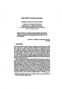
tr, if (l, v) − → (l 00 , v00 ), with v00 ∈ z00 , then ∀v0 in z, ∃tr0 .(l, v0 ) −→ (l 00 , v), ˜ with untime(tr0 ) = untime(tr) 00 and v˜ ∈ z . According to the construction given in algorithm 1, for a particular location of the timed automaton, the zones corresponding to any two nodes are disjoint. Convexity of the zones and pre-stability property together ensure that a zone with elapse of time is intercepted by a single hyperplane of the form x = h as in the case of regions, where x ∈ C and h ∈ N. Some approaches for preserving convexity and implementing pre-stability have been discussed in [21]. As an example consider the timed automaton in l0 {x} x ≤ 4 a

l2

z5

y=7 z2

l1 x>5 b ∧y >7

z6

y

4

z3

z4

z1

2 0

x=5

x

Figure 1: A timed automaton and the zones for location l1 Figure 1. The zones corresponding to location l1 as produced through algorithm 1 are shown in the right side of the figure. A similar construction of zone graph has also been used in [11]. In the construction used in [11], in the final phase, the nodes corresponding to a particular location with zones that are time abstracted bisimilar to each other are merged as long as the merged zone is convex. Though this may reduce the number of zones in the final zone graph, the operation itself is exponential in the number of clocks of the timed automaton. Due to the absence of this merging phase in the algorithm described in this paper, while checking the existence of the relations following the method described here, one may need to consider more pairs of states, but we expect this overhead to be less compared to the expensive operation of merging the nodes with time abstracted bisimilar zones.

S. Guha, S. N. Krishna, C. Narayan & S. Arun-Kumar

51

Algorithm 1 Construction of Zone Graph Input: Timed automaton A Output: Zone graph corresponding to A 1: Calculate maxxl for each location l ∈ L and each clock x ∈ C. This is required for abstraction to ensure finite 2: 3: 4: 5: 6: 7: 8: 9: 10: 11: 12: 13: 14: 15: 16: 17: 18: 19: 20: 21: 22: 23: 24: 25: 26: 27: 28:

number of zones in the zone graph. Initialize Q to an empty queue. Enqueue(Q, < l0 , 0/ >). successors added = f alse. while Q not empty do < l, l p >= dequeue(Q) if l p 6= 0/ then, g,a,X 0

For the edge l p −−−→ l in A, for each existing zone zl p of l p , create the zone z = (zl p ↑ ∩ g[X 0 ←0] ) of l, when z 6= 0. / Abstract each of the newly created zones if necessary and for any newly created zone z, for location l, if ∃z1 of same location such that z ∩ z1 6= 0, / then merge z and z1 . Update edges from zones of l p to zones of l appropriately. If a new zone of l is added or an existing zone of l is modified, then for all successors l j of l, enqueue < l j , l > to Q. successors added := true. end if . flag set to false when the canonical decomposition does not produce further zones new zone l := true. while new zone l do Split the existing zones z of l based on the canonical decomposition of the guards on the outgoing edges of l . It is not always necessary for a split to happen. For every zone z of l, consider z ↑ and split it further based on the canonical decomposition of the guards on the outgoing edges of l . Note that the zones created from this split are convex. Abstract each of the newly created zones if necessary and update edges appropriately. If new zones are not created then set new zone l to f alse. end while if any new zones of l are created or any existing zones of l are modified due to the canonical decomposition of the outgoing edges of l and successors added = f alse then for all the successor locations l j of l to Q, enqueue < l j , l > to Q. end if end while /* Phase 2 : In this phase, pre-stability is enforced */ new zone = true while new zone do new zone = f alse g,a,X 0

29: 30:

do 31: 32: 33: 34: 35: 36: 37:

. Every element is a pair consisting of a location and its parent . flag set to true whenever successors of a location are added to Q

for all edges li −−−→ l j do α for all pairs of zones zlik , zl jm such that zlik − → zl jm is an edge in the zone graph where α ∈ Act ∪ R≥0

if zlik is not pre-stable with respect to zl jm , then Split zlik to make it pre-stable with respect to zl jm . . Note that this split still maintains convexity of zlik since the zone is split entirely along an axis that is parallel to the diagonal in the |C|-dimensional space. new zone := true Update the edges end if end for end for end while

52

Relations for Timed Automata

3

Equivalences for Timed Systems

In this section, we define the timed and the time abstracted relations considered in this work. We only consider the strong form of these relations here. We enumerate a few clauses first using which we define p1 R p2 where p1 and p2 are two timed automata states and R is a timed or a time abstracted relation. a

a

1. ∀a ∈ Act ∧ ∀p01 , p1 → p01 ⇒ [ ∃p02 : p2 → p02 ∧ p01 R p02 ] a a 2. ∀a ∈ Act ∧ ∀p02 , p2 → p02 ⇒ [ ∃p01 : p1 → p01 ∧ p01 R p02 ] d a

a

3. ∀a ∈ Act ∧ ∀p01 , p1 → p01 ⇒ [ ∃p02 ∃d ∈ R≥0 : p2 →→ p02 ∧ p01 R p02 ] d

a

a d

4. ∀a ∈ Act ∧ ∀p01 , p1 → p01 ⇒ [ ∃p02 ∃d1 , d2 ∈ R≥0 : p2 →1 →→2 p02 ∧ p01 R p02 ] d

d

5. ∀d ∈ R≥0 ∧ ∀p01 , p1 → p01 ⇒ [ ∃p02 : p2 → p02 ∧ p01 R p02 ] d

d0

6. ∀d ∈ R≥0 ∧ ∀p01 , p1 → p01 ⇒ [ ∃p02 ∃d 0 ∈ R≥0 : p2 → p02 ∧ p01 R p02 ] d

d0

d

d0

7. ∀d ∈ R≥0 ∧ ∀p01 , p1 → p01 ⇒ [ ∃p02 ∃d 0 ∈ R≥0 ∧ d ≤ d 0 : p2 → p02 ∧ p01 R p02 ] 8. ∀d ∈ R≥0 ∧ ∀p02 , p2 → p02 ⇒ [ ∃p01 ∃d 0 ∈ R≥0 ∧ d ≥ d 0 : p1 → p01 ∧ p01 R p02 ]

R is a timed simulation if the clauses 1 and 5 hold. For each (p1 , p2 ) ∈ R, p2 time simulates p1 . R is a timed simulation equivalence if p1 time simulates p2 and p2 time simulates p1 . A symmetric timed simulation is a timed bisimulation relation. A symmetric relation that satisfies clauses 1 and 6 is a time abstracted bisimulation. A relation that is symmetric and satisfies clauses 3 and 6 is a time abstracted delay bisimulation relation. A symmetric relation satisfying clauses 4 and 6 is a time abstracted observational bisimulation. A timed performance prebisimulation relation [11] satisfies the clauses 1, 2, 7 and 8. The corresponding largest bisimulation relations are called bisimilarity relations and they are timed bisimilarity (∼t ), time abstracted bisimilarity (∼u ), time abstracted delay bisimilarity (∼y ), time abstracted observational bisimilarity (∼o ) whereas the largest prebisimulation relation is called timed performance prebisimilarity (-). p - q denotes that p is at least as fast as q. It is easy to see from the definitions that timed bisimilarity implies time-abstracted bisimulation whereas the converse is not true. Besides, the definitions imply ∼u ⊆ ∼y ⊆ ∼o . Also the existence of a bisimulation relation between two states implies the existence of the corresponding simulation equivalence and timed performance prebisimilarity lies in between timed bisimulation and time abstracted bisimulation. Hence we have ∼t ⊆ - ⊆ ∼u ⊆ ∼y ⊆ ∼o and similar containment relations also exist among the corresponding simulation equivalences.

4

Deciding Relations for Timed Automata

In this section, we present a unifying approach to decide several relations for timed automata using the zone graph constructed in algorithm 1.

4.1

Deciding Timed Bisimulation

Timed bisimulation has been proven to be decidable for timed automata [4]. A product construction technique on the region graphs has been used in [4] whereas in [22], a product construction is applied on zone graphs instead for deciding timed bisimulation. Though decidable, timed bisimulation may have uncountably many equivalence classes[2]. We define corner point bisimulation relation and show that corner point bisimulation coincides with timed bisimulation. With corner point bisimulation, only a finite

S. Guha, S. N. Krishna, C. Narayan & S. Arun-Kumar

53

number of pairs of corner points are needed for bisimilarity checking. Further, our method eliminates the product construction on zone graphs. Let A, B be timed automata having CA ,CB as the respective maximum constants used in the constraints appearing in the two automata. Let p and q be two states in T (A) and T (B) respectively. We show that (i) if p and q are initial states, or states where all clock valuations are integers, then timed bisimulation for p, q can be decided by checking delays of the form n, n + δ or n − δ , where n ∈ {0, 1, . . . ,C}, C = max(CA ,CB ), and δ is a symbolic value for an infinitesimal positive quantity. (ii) If there is some clock y having a non-zero rational fractional part, then along with the delays of the form mentioned above, we check delays of the form f , f + δ or f − δ , with f = 1 − f rac(v(y)), f rac(v(y)) is the fractional part of the value of clock y. Delays of the form mentioned above are called corner point delays or cp-delays. We define corner point bisimulation formally below. Definition 2. 1. Corner point simulation (cp-simulation): A relation R is a corner point simulation relation, if for every pair of timed automata states (p, q) ∈ R, the following conditions hold. a a (i) For every visible action a ∈ Act, if p → − p0 , then ∃q0 such that q → − q0 and p0 Rq0 d (ii) Considering the maximum possible delay d from p, if p → − p0 and p0 is in node N (p), then d

∃q0 such that q → − q0 and p0 Rq0 ε (iii) For every node N (p0 ) 6= N (p) such that N (p) → − N (p0 ), considering the minimum delay d

d

d from p, if p → − p0 , then ∃q0 such that q → − q0 and p0 Rq0

Here q cp-simulates p. A symmetric corner point simulation relation is a corner point bisimulation (cp-bisimulation). 2. Corner point trace: A timed trace from a state p to p0 , where all the delays are cp-delays is called a corner point trace. Lemma 1. For checking whether the timed automata states p and q are related through corner point simulation or corner point bisimulation relation, there are only finitely many pairs of states that need to be considered. This is due to the fact that for any (p, q) ∈ R, R being a cp-bisimulation relation, the valuations of all the clocks appearing in both p and q are of the form n, n + δ or n − δ , where n ∈ {0, 1, . . . ,CA } or n ∈ {0, 1, . . . ,CB }. If p ∈ T (A) and q ∈ T (B), then CA and CB are the maximum constants appearing in A and B respectively. Theorem 1. Corner point simulation and corner point bisimulation relations are decidable. Theorem 2. For two timed automata states p and q, 1. p ∼t q ⇒ pRq, where R is a corner point bisimulation relation. 2. pRq ⇒ p ∼t q, where R is a corner point bisimulation relation. 3. p and q are timed bisimilar if and only if p and q are cp-bisimilar. Theorem 2 shows that the decidability of cp-bisimulation is sufficient for timed bisimulation. Synthesis of Distinguishing Formulae. Given two timed automata A and B which are not timed bisimilar, we propose a technique that synthesizes a formula that captures the differences between A and B. In [14], a characteristic formula for timed automata has been defined using a certain fragment of the µ-calculus presented in [12]. Timed bisimilarity between two timed automata is decided by comparing

54

Relations for Timed Automata

one timed automaton with the characteristic formula of the other. A characteristic formula is a significantly complex formula describing the entire behaviour of the timed automaton. Here we describe how we can in general generate a simpler formula using a fragment of the logic described in [14]. The logic we use for generating the distinguishing formula has been described in [1] which is a timed extension of Hennessy-Milner logic and does not contain any recursion as opposed to the logic used in [14]. The set Mt of Hennessy-Milner logic formulae with time over a set of actions Act, set D of formula clocks (distinct from the clocks of any timed automaton) is generated by the abstract syntax φ ::= tt | ff | φ ∧ ψ | φ ∨ ψ | haiφ | [a]φ | ∃∃φ | ∀∀φ | x in φ | g where a ∈ Act, x ∈ D and g ∈ B(D). The logic used in [10] for constructing distinguishing formula uses an explicit negation rather than using the operators [ ] and ∀∀. Besides a distinguishing formula in [10] uses real delays whereas in our case, the formula clock values are compared with integers. Also the distinguishing formula synthesized in [10] considers the entire branching structure of the given automata whereas in our case, the formula is synthesized from the moves in a game and is thus more succinct. Given a timed automaton A, Mt is interpreted over an extended state h(l, v)ui, where (l, v) is a state of A and u is a time assignment of D. Transitions between the extended states are defined by: d a a h(l, v)ui → − h(l, v + d)u + di and h(l, v)ui → − h(l 0 , v0 )u0 i iff h(l, v)i → − h(l 0 , v0 )i and u = u0 . ∃∃φ holds in an extended state if there exists a delay transition leading to an extended state satisfying φ . Similarly ∀∀ denotes universal quantification over delay transitions, and hai and [a] respectively denote existential and universal quantification over a-transitions. The formula x in φ introduces a formula clock x and initializes it to 0, i.e. h(l, v)ui |= x in φ =⇒ h(l, v)u[x←0] ¯ i |= φ . The formula clocks are used in formulas of the form g which is satisfied by an extended state if the values of the formula clocks used in g satisfy the specified relationship. A formula is said to be closed if each occurrence of a formula clock x is within the scope of an x in construct. While checking cp-bisimulation, we describe below a method to generate a closed formula in Mt that distinguishes two timed automata that are not timed bisimilar. For constructing the formula, we consider a cp-bisimulation game between the initial states of the timed automata which can be thought of as a bisimulation game (see [19]) for deciding timed bisimulation between two timed automata. The game is played between two players, the challenger and the defender. Each round of the game consists of the challenger choosing one of the zone graphs and making a move as defined in the definition of the cp-bisimulation relation. The defender tries to replicate the move in the other zone graph. The defender loses the game if after a finite sequence of rounds, the challenger makes a move on one zone graph which the defender cannot replicate on the other. If the defender loses the game, we look at the sequence of moves chosen by the challenger to construct the distinguishing formula as follows: Given two timed automata A and B (with C1 ∩C2 = 0/ where C1 and C2 are clocks of A and B respectively) and their zone graphs being ZA and ZB , let us suppose without loss of generality that the challenger makes a move on ZA in the first round. We derive a formula from the moves of the game which is satisfied by automaton A and not by automaton B. The set of formula clocks are disjoint from the clocks in A and B. The distinguishing formula ζ is initialized to x1 in () with the introduction of a formula clock x1 . Corresponding to every clock y in C1 ∪ C2 , there exists a clock x ∈ D such that their valuations are the same, i.e. v(y) = v(x). We can define a mapping η : C1 ∪C2 → D. With the introduction of the formula clock x1 mentioned above, we have ∀y ∈ C1 ∪ C2 , η(y) = x1 . Whenever one or more clocks are reset either in A or B corresponding to the visible actions chosen by the challenger and the defender, a new formula clock is introduced. If U ⊆ C1 and V ⊆ C2 be the subset of clocks reset for actions chosen in a particular round, then a new formula clock xi is introduced such that ∀y ∈ U ∪V, η(y) = xi . Subformulas

S. Guha, S. N. Krishna, C. Narayan & S. Arun-Kumar

a

l1 b {x}

l

a

l2 b b{x} l4 {x} l5 l3 c c c c c l6 l l l 8 9 x ≤ 1 d 7d d d x ≤ 1 dl10 x≤1 l11 l13 l12 l14 l15

55

a

L

L1 {y} b b{y} L3 L2 c c c L4 L5 L6 y ≤ 1d d y ≤ 1 d L9 L7 L8

Figure 2: Example of distinguishing formula in Mt of ζ are always added to the scope of the innermost or the last added clock in ζ . The subformulas of ζ are added based on the move of the challenger as described below. - The challenger performs action a ∈ Act in ZA (ZB ). If the defender can reply with a in ZB (ZA ) and in either of the moves at least one clock is reset in the corresponding timed automata, then add hai x in ( ) ( [a] x in ( ) ) to the innermost scope of ζ , where x is a new formula clock. If no clock is being reset, then simply add hai([a]) to the innermost scope of ζ . If the defender cannot reply to the move of the challenger, then append haitt ( [a]ff ) in the innermost scope and declare ζ to be the distinguishing formula. - The challenger performs a delay d in ZA (ZB ), where the delays are as defined in the cp-bisimulation relation, i.e. cp-delays and it reaches a state with clock valuation v. For every clock y in ZA (ZB ), we construct a subformula as follows: if v(y) = n is an integer, then construct the subformula x = n, where x is η(y). If v(y) is of the form n + δ , where n ∈ N, then construct the subformula n < x < n+1 and if v(y) is of the form n−δ , then construct the subformula n−1 < x < n. Conjunct all these subformulas to obtain ψ and append ∃∃(ψ) ( ∀∀(ψ) ) to the innermost scope of ζ .

Note that in ζ , the subformulas of the form g define the smallest set of extended states reachable along the trace followed in ZA that can be specified by subformulas of the form g. In the two timed automata shown in Figure 2, the moves of the challenger are marked by a X mark. The challenger starts making a move from the automaton on the left and hence we construct a formula in Mt that is satisfied by the automaton on the left but not by the automaton on the right. Following the steps mentioned above, we obtain the formula x1 in (hai[b] x2 in (hci ∃∃(1 < x2 < 2 ∧ hditt))). We note that though the cp-bisimulation relation can be decided between any two timed automata states with arbitrary clock valuation, the distinguishing formula is constructed only while checking the relation between the initial states of the two timed automata. The technique described here to check for lack of timed bisimilarity can be adapted to many of the other relations studied in this paper. Our prototype tool implementation which is currently underway will also incorporate them.

4.2

Deciding Timed Performance Prebisimulaton

In this section, we define corner point prebisimulation relation and show that this relation coincides with the timed performance prebisimulation relation. We use the zone graph constructed according to algorithm 1 for checking corner point prebisimulation. Unlike the case of timed bisimulation, a product construction on zone graphs is not useful for deciding timed performance prebisimulation relation : for example, consider two simple timed automata with clocks x and y respectively, each with two locations and one edge between them such that the edge in one automaton is labelled with hx = 2, a, 0i / while the

56

Relations for Timed Automata

other is labelled with hy = 5, a, 0i. / These two timed automata are timed performance prebisimilar though a product on the region graphs of these two automata does not produce an action transition and thus does not have sufficient information to show that one of the automata can actually perform action a following a lesser delay. We define the corner point prebisimulation relation in terms of a two player game that is similar to the bisimulation game. The game is played between two players, challenger and defender on the zone graphs (as constructed in algorithm 1) of two timed automata. In each round, the challenger chooses a side and the defender chooses the other side. After selecting a side, the challenger can either perform a visible action or a delay action. Note that in the corner point prebisimulation relation, the delays are cp-delays as given by Definition 2. Two timed automata states p and q in T (A) and T (B) respectively are cp-prebisimilar, denoted p -cp q, if starting from p and q, the defender wins and the cp-delay moves in A are less than or equal to the corresponding cp-delay moves in B. We write A -cp B if p -cp q, where p and q are respectively the initial states of T (A) and T (B). We now explain the possible moves of the game on the respective zone graphs Z(A,p) and Z(B,q) . Each move results in a new state in a possibly new zone from which the next move is made in the next round. - (Challenger chooses T (A) (Move 1)): Performs a visible action a ∈ Act. (Defender chooses T (B)): i) Performs the same action a. - (Challenger chooses T (A) (Move 2)): Performs maximum delay d and stays inside the same zone. (Defender chooses T (B)): i) Performs delay d. - (Challenger chooses T (A) (Move 3)): Performs the minimum delay d and moves to the next zone. (Defender chooses T (B) and performs one of the following delays): i) delay d or ii) cp-delays d 0 ≥ d that take q to the delay successor zones. - (Challenger chooses T (B) (Move 1)): Performs a visible action a ∈ Act. (Defender chooses T (A)): i) Performs the same action a.

- (Challenger chooses T (B) (Move 2)): Performs maximum delay d and stays inside the same zone. (Defender chooses T (A) and performs one of the following delays): i) delay d itself or ii) Consider cp-delay d 0 ≤ d, such that p on elapsing d 0 reaches the end of the same zone or other delay successor zones. - (Challenger chooses T (B) (Move 3)): Performs the minimum delay d and moves to the next zone. (Defender chooses T (A) and performs one of the following delays): i) delay d itself or ii) cpdelays d 0 ≤ d such that p on elapsing d 0 reaches the beginning of the delay successor zones or iii) cp-delays d 0 ≤ d such that it reaches the end of the same or other delay successor zones. Figure 3 illustrates how a corner point prebisimulation game is played between the challenger and the defender and shows each of the moves described above. Note that in automata A and B, for locations l0 and L0 respectively, - action a is enabled at all delays. - actions a and b, both are enabled when x ≤ 12 and y ≤ 15 respectively and - action c is enabled in the interval 12 < x ≤ 16 in A and in the interval 15 < y < 22 in B. For these two automata, we can see that (l0 , x = 0) - (l1 , y = 0), i.e. the automaton A is at least as fast as automaton B. In A, the zones created using the algorithm 1 corresponding to l0 are x ≤ 4, 4 < x ≤ 12, 12 < x ≤ 16 and x > 16, whereas in B, the zones created are y ≤ 11, 11 < y ≤ 15, 15 < y < 20, 20 ≤ y < 22 and y ≥ 22. In Figure 3, we also show a representative diagram of these zones. The dots on the axis of the clock denote the boundary of a zone that does not signify any change in behaviour whereas the

S. Guha, S. N. Krishna, C. Narayan & S. Arun-Kumar

l3

12

l4

16

11 y ≤ 15

4 x>

y>

L1 y

L2

0

(a) Timed Automaton A

a

y
0, n < k

Other parameters remaining the same, if the defender wins the game with more number of rounds, then it also wins the game which has a smaller number of rounds in the game. ha/d,a/di

ha/d ,a/d i,(Z ,≤)

Lemma 4. n − Γk −→ n − Γk 1 2 A . ha/d,a/di ha/d ,a/d i,(Z ,≤) ha/d ,a/d i,(Z ,≤) n − Γk −→ n − Γk 1 2 A ∨ n − Γk 1 2 B

The first half of the above lemma states that all the parameters remaining the same, if the defender can always reply with an exact delay, then the defender can reply with a delay d2 in ZA such that d2 ≤ d1 and it can reply with a delay d2 in ZB such that d1 ≤ d2 . This also leads to the fact that all the parameters remaining the same, if the defender wins the cp-bisimulation game, then it also wins the cp-prebisimulation game. ha/d,a/di

Lemma 5. n − Γk

ha/ε,a/εi

−→ n − Γk

ha/ε,ε.a/εi

−→ n − Γk

ha/ε,ε.a.ε/εi

−→ n − Γk

If the defender can match a delay action exactly as in the corner point bisimulation, then it can match an epsilon move of the challenger. Also if the defender can reply to a visible action of the challenger, then it can reply with an ε.a or an ε.a.ε move since ε represents delay including zero delay.

5.3

Infinite Game Hierarchy

On assigning different values to the parameters n, k, G, α and β in the game template and using the lemmas given in subsection 5.2, we can generate an infinite game hierarchy which is shown in Figure 4(c). The dashed lines in the figure denote that if the defender has a winning strategy for a game with infinitely many rounds or alternations, then it also wins a game with a finite number of rounds or alternations. Figure 4(b) shows the hierarchy of the games that correspond to the timed relations in Figure 4(a). The diagram in Figure 4(b) is only a small part of the entire hierarchy of timed games and this leaves us with the scope of studying several timed relations that are not present in the existing literature.

6

Conclusion

In this paper, we present a unified zone based approach to decide various timed relations between two timed automata states. In our method, we do not need the product construction on regions or zones for deciding these relations as done in [4] or [22]. We also provide a game semantics for deciding these timed relations and show that the hierarchy among the games reflects the hierarchy among the relations. The advantage of a game-theoretic formulation is that it allows fairly general relationships between the parameters on Γ to define the hierarchy. The fine-tuning and variations of these parameters allow formulations of many more equivalences and preorders than the ones present in the literature related to behavioural equivalences involving real time which otherwise may not be easily captured through operational definitions and reasoning. Unlike existing approaches which check if two timed automata states are related through some relation, our game approach also allows generating a distinguishing formula that guides us to find a path in one of the zone graphs which was responsible for the relation not

S. Guha, S. N. Krishna, C. Narayan & S. Arun-Kumar

61

Timed Bisimulation Timed Sim. Equivalence

Timed Performance Prebisimulation

Γha/d,a/di ∞

Timed Abstracted Bisimulation Time Abstracted Sim. Equivalence Timed Abstracted Delay Bisimulation Time Abstracted Delay Sim. Equivalence Timed Abstracted Obs. Bisimulation Time Abstracted Delay Sim. Equivalence (a)

1 ,a/d2 i,(ZA ,≤) Γha/d ∞

n − Γha/d,a/di ∞ (n−1)−Γha/d,a/di ∞

...

... ...

ha/d,a/di

(n−1)−Γk

...

ha/ε,ε.a/εi ... Γ∞ ... Γha/ε,ε.a.ε/εi ∞ ...

1 ,a/d2 i,(ZA ,≤) n − Γha/d ∞

...

ha/d,a/di

n − Γk

ha/d,a/di

n−Γk−1

Γha/ε,a/εi ∞

... ...

ha/d1 ,a/d2 i,(ZA ,≤)

n−Γk

ha/ε,a/εi

... . .. ha/d,a/di

(n−2)−Γk

ha/d,a/di

ha/d,a/di

(n−1)−Γk−1

... .. .. . . ...

n−Γk−2

... .. .. . .

ha/d,a/di

0 −Γ1 ha/d,a/di Γ∞

ha/d1 ,a/d2 i,(ZA ,≤) 0−Γha/d,a/di ∞ Γ∞ 1 ,a/d2 i,(ZB ,≤) ∨ Γha/d ∞

0−Γha/ε,a/εi ∞ 0−Γha/ε,a/εi ∞ 0−Γha/ε,a/εi ∞

Figure 4: games

ha/ε,a/εi Γ∞

Γha/ε,ε.a/εi ∞

... .. n−Γha/ε,ε.a.ε/εi k . ... ...

n−Γk−1 1

... .. .. . .

... .. .. . .

...

ha/d,a/di ha/d,a/di

ha/ε,ε.a/εi

n−Γk

ha/d ,a/d2 i,(ZA ,≤)

(n−1)−Γk

... .. .. . .

1 −Γ2

0 −Γ2

ha/d1 ,a/d2 i,(ZA ,≤)

n−Γk

...

ha/d1 ,a/d2 i,(ZA ,≤)

1−Γ2

ha/d1 ,a/d2 i,(ZA ,≤)

0−Γ2

ha/d1 ,a/d2 i,(ZA ,≤)

0−Γ1

(c)

ha/ε,a/εi

1−Γ2

...

ha/ε,a/εi

1−Γ2

ha/ε,a/εi

0−Γ2

0−Γ2 0−Γ1

...

ha/ε,ε.a/εi ha/ε,ε.a/εi

1−Γ2

ha/ε,ε.a/εi

0−Γ2

0−Γ1

ha/ε,ε.a.ε/εi

ha/ε,ε.a.ε/εi ha/ε,ε.a.ε/εi

0 − Γ1

ha/ε,ε.a.ε/εi Γ∞

(b)

Relations over timed automata, game characterization and the infinite hierarchy of timed

holding good between the corresponding states. Identifying this path helps us to refine appropriately an implementation that should conform to a given specification through the relation. As further work, we plan to extend the game semantics to relations over probabilistic extensions to timed automata [13]. We would also like to investigate the applicability of our zone graph construction for deciding these relations.

References [1] L. Aceto, A. Ingolfsd ´ ottir, ´ K.G. Larsen & J. Srba (2007): Reactive Systems: Modelling, Specification and Verification. Cambridge University Press, doi:10.1145/1811226.1811243. [2] R. Alur, C. Courcoubetis & T. A. Henzinger (1994): The Observational Power of Clocks. In: Proceedings of CONCUR, pp. 162–177, doi:10.1007/BFb0015008. [3] R. Alur & D.L. Dill (1994): A Theory of Timed Automata. Theoretical Computer Science 126, pp. 183–235, doi:10.1016/0304-3975(94)90010-8. [4] K. Cerans (1992): Decidability of bisimulation equivalences for parallel timer processes. In: Proceedings of CAV, 663, Springer-Verlag, pp. 302–315, doi:10.1007/3-540-56496-9 24.

62

Relations for Timed Automata

[5] X. Chen & Y. Deng (2008): Game Characterizations of Process Equivalences. In: Proceedings of APLAS, pp. 107–121, doi:10.1007/978-3-540-89330-1 8. [6] C. Daws & S. Tripakis (1998): Model Checking of Real-Time Reachability Properties Using Abstractions. In: Proceedings of TACAS, Springer-Verlag, pp. 313–329, doi:10.1007/BFb0054180. [7] E. Fleury G. Behrmann, P. Bouyer & K. G. Larsen (2003): Static guard analysis in timed automata verification. In: Proceedings of TACAS, Springer-Verlag, pp. 254–270, doi:10.1007/3-540-36577-X 18. [8] K. G. Larsen G. Behrmann, P. Bouyer & R. Pelanek (2006): Lower and upper bounds in zone-based abstractions of timed automata. International Journal on Software Tools for Technology Transfer 8, pp. 204–215, doi:10.1007/s10009-005-0190-0. [9] Rob J. van Glabbeek (1990): The Linear Time-Branching Time Spectrum (Extended Abstract). In: Proceedings of CONCUR, pp. 278–297, doi:10.1007/BFb0039066. [10] J. C. Godskesen & K. G. Larsen (1995): Synthesizing distinguishing formulae for real time systems. Nordic J. of Computing 2(3), pp. 338–357. [11] S. Guha, C. Narayan & S. Arun-Kumar (2012): On Decidability of Prebisimulation for Timed Automata. In: Proceedings of CAV, Springer-Verlag, pp. 444–461, doi:10.1007/978-3-642-31424-7 33. [12] T. A. Henzinger, X. Nicollin, J. Sifakis & S. Yovine (1992): Symbolic Model Checking for Real-time Systems. Information and Computation 111, pp. 394–406, doi:10.1006/inco.1994.1045. [13] M. Kwiatkowska, G. Norman, R. Segala & J. Sproston (2002): Automatic verification of real-time systems with discrete probability distributions. Theoretical Computer Science 282(1), pp. 101–150, doi:10.1016/S0304-3975(01)00046-9. [14] F. Laroussinie, Kim G. Larsen & C. Weise (1995): From Timed Automata to Logic – and Back. In: Proceedings of MFCS, pp. 529–539, doi:10.1007/3-540-60246-1 158. [15] F. Laroussinie & Ph. Schnoebelen (2000): The State Explosion Problem from Trace to Bisimulation Equivalence. In: Proceedings of FoSSaCS, Springer-Verlag, pp. 192–207, doi:10.1007/3-540-46432-8 13. [16] K. G. Larsen & W. Yi (1994): Time abstracted bisimulation: implicit specifications and decidability. In: Proceedings of MFPS, 802, Springer-Verlag, pp. 160–176, doi:10.1007/3-540-58027-1 8. [17] R. Milner (1989): Communication and Concurrency. Prentice Hall. [18] C. Stirling (1995): Local Model Checking Games. In: Proceedings of CONCUR, pp. 1–11, doi:10.1007/3540-60218-6 1. [19] C. Stirling (2001): Modal and temporal properties of processes. Springer-Verlag New York, Inc., New York, NY, USA, doi:10.1007/978-1-4757-3550-5. [20] H. Straubing (1994): Finite automata, formal logic, and circuit complexity. Birkhauser Verlag, Basel, Switzerland, Switzerland, doi:10.1007/978-1-4612-0289-9. [21] S. Tripakis & S. Yovine (2001): Analysis of Timed Systems using Time-Abstracting Bisimulations. Formal Methods in System Design 18, pp. 25–68, doi:10.1023/A:1008734703554. [22] C. Weise & D. Lenzkes (1997): Efficient scaling-invariant checking of timed bisimulation. In: Proceedings of STACS, 1200, Springer, Berlin, pp. 177–188, doi:10.1007/BFb0023458.