Adaptive Boundary Element Methods

Noname manuscript No. (will be inserted by the editor)

Adaptive Boundary Element Methods A posteriori error estimators, adaptivity, convergence, and implementation

arXiv:1402.0744v1 [math.NA] 4 Feb 2014

Michael Feischl · Thomas Fuhrer ¨ · Norbert Heuer · Michael Karkulik · Dirk Praetorius

Received: date / Accepted: date

Abstract This paper reviews the state of the art and discusses very recent mathematical developments in the field of adaptive boundary element methods. This includes an overview of available a posteriori error estimates as well as a state-of-the-art formulation of convergence and quasi-optimality of adaptive mesh-refining algorithms. Keywords boundary element method · a posteriori error estimate · adaptive mesh refinement · convergence · optimal complexity Mathematics Subject Classification (2000) 65N30 · 65N38 · 65N50 · 65R20 · 41A25

The research of MF, TF, and DP is supported by the Austrian Science Fund (FWF) through the research project Adaptive boundary element method, funded under grant P21732, see http://www.asc.tuwien.ac.at/abem/. In addition, the authors MF and DP acknowledge support through the FWF doctoral program Dissipation and dispersion in nonlinear PDEs, funded under grant W1245, see http://npde.tuwien.ac.at/. The research of NH is supported by CONICYT projects Anillo ACT1118 (ANANUM) and Non-conforming boundary elements and applications, funded under grant Fondecyt 1110324. The research of MK is supported by the CONICYT project Efficient adaptive strategies for nonconforming boundary element methods, funded under grant Fondecyt 3140614. M. Feischl, T. F¨uhrer, and D. Praetorius Institute for Analysis and Scientific Computing Vienna University of Technology Wiedner Hauptstrasse 8-10, 1040 Wien, Austria E-mail: {michael.feischl,thomas.fuehrer, dirk.praetorius}@tuwien.ac.at N. Heuer and M. Karkulik Facultad de Matem´aticas Pontificia Universidad Cat´olica de Chile Avenida Vicu˜na Mackenna 4860, Santiago, Chile E-mail: {nheuer,mkarkulik}@mat.puc.cl

Contents 1 2 3 4 5 6 7 8 9 10

Introduction . . . . . . . . . . . . . . . . . . . . . . Mathematical foundation of the BEM . . . . . . . . Localization of fractional order Sobolev norms . . . A posteriori error estimators for the h-version . . . . A posteriori error estimators for the p and hp-versions Estimator reduction . . . . . . . . . . . . . . . . . . Mesh refinement . . . . . . . . . . . . . . . . . . . . Optimal convergence of adaptive BEM . . . . . . . . Implementational details . . . . . . . . . . . . . . . Conclusion . . . . . . . . . . . . . . . . . . . . . .

. . . . . . . . . .

. . . . . . . . . .

. . . . . . . . . .

. . . . . . . . . .

1 7 14 18 39 43 52 56 68 73

1 Introduction Many practically relevant PDEs1 on bounded or unbounded domains Ω ⊂ Rd can be equivalently formulated as integral equations on the (d − 1)-dimensional boundary Γ = ∂ Ω . This reformulation is then discretized and solved numerically by BEM2 . Striking advantages of BEM over FEM3 rely on the dimension reduction, the natural treatment of unbounded domains, as well as a potentially high rate of convergence with respect to both, the natural energy norm as well as the pointwise error. On the other hand, high convergence rates are only achieved if the (given) data as well as the (unknown) exact solution are sufficiently smooth or if the possible singularities are appropriately resolved. In practice, one thus observes a huge gap between the theoretically possible optimal rate and the empirical convergence behavior, if the meshes are refined uniformly. The remedy is to use appropriately graded meshes which resolve the possible singularities of data and exact solution. To this end, a posteriori error estimation and related adaptive mesh-refinement have themselves proven to be important tools for scientific 1 2 3

partial differential equation (PDE) boundary element method (BEM) finite element method (FEM)

2

M. Feischl, T. F¨uhrer, N. Heuer, M. Karkulik, D. Praetorius

computing, cf. [3,145]. First, they allow to monitor the actual error and to stop the computation if the computed solution is accurate enough. Second, they may also drive the problem-adapted discretization and thus the appropriate resolution of the possible singularities. While the convergence and quasi-optimality of AFEM4 has been mathematically analyzed within the last decade [26,46,56,110,139], analogous results for ABEM5 [7,65,66,70,76] have only been achieved very recently, see also [52,75,77,103] for adaptive wavelet-based BEM.

1.1 Galerkin BEM and C´ea lemma Throughout, our main focus is on Galerkin BEM. Here, the mathematical frame reads as follows: Let X be a real Hilbert space with norm k·kX , which will be an appropriate Sobolev space in the applications in mind. Let b : X × X → R be a continuous and elliptic bilinear form, i.e., there are constants Ccont ,Cell > 0 such that b(v, w) ≤ Ccont kvkX kwkX

for all v, w ∈ X

(1)

and b(v, v) ≥ Cell kvk2X

for all v ∈ X .

(2)

Given a linear and continuous functional F : X → R, the so-called weak formulation (or variational formulation) of the BIE6 reads: Find the exact solution u ∈ X of b(u, v) = F(v) for all v ∈ X .

(3)

Based on a triangulation T of the underlying spatial domain, let XT ⊂ X be a finite-dimensional subspace. The Galerkin BEM discretization reads: Find U ∈ XT such that b(U,V ) = F(V ) for all V ∈ XT .

(4)

For both, the continuous as well as the discrete formulations (3) and (4), the Lax-Milgram lemma applies and proves the existence and uniqueness of u ∈ X resp. U ∈ XT . Moreover, a direct computation with the Galerkin orthogonality b(u − U,V) = 0

for all V ∈ XT ,

(5)

provides the C´ea lemma Cell ku − UkX ≤ min ku − VkX ≤ ku − UkX V ∈XT Ccont

(6)

i.e., the computable Galerkin solution U ∈ XT is a quasibest approximation of u among all functions V in the discrete space XT . 4 5 6

adaptive finite element method (AFEM) adaptive boundary element method (ABEM) boundary integral equation (BIE)

1.2 Adaptive algorithm As a consequence of the C´ea lemma (6), a natural question is how to choose the discrete space XT (resp. the mesh T ). Ideally, one should choose the discrete space XT such that the best approximation error in (6) is minimal with respect to the number of degrees of freedom. Usually the necessary a priori knowledge is not available (even if the generic singularities appear to be known), such that it is infeasible to address this question. Another possibility is to choose a sequence of meshes such that the best approximation error shows an “optimal decay” with increasing dimension of XT . Usually this question is empirically addressed by adaptive algorithms which start from an initial mesh T0 and generate a sequence of (locally) refined meshes Tℓ for ℓ ∈ N0 by iterating the loop solve →

estimate →

mark → refine . (7)

It provides a sequence of Galerkin solutions Uℓ ∈ Xℓ := XTℓ with nested discrete spaces Xℓ ⊂ Xℓ+1 ⊂ X for all ℓ ≥ 0. Adaptive algorithms thus work with a sequence of meshes and need to solve in every step. Yet, it can be observed in model problems that they outperform algorithms which uniformly refine a coarse mesh up to a given number of degrees of freedom and finally solve only once. This superiority appears in terms of memory versus error as well as time consumption versus error, cf. [4,10]. The module solve consists of the direct or iterative solution of the linear system corresponding to (4) to compute the (approximate) Galerkin solution Uℓ ∈ Xℓ . Mathematical questions arise from the fact that, first, BEM matrices are densely populated (i.e., the number of non-zero entries is roughly equivalent to the overall number of entries) and hence have to be treated by matrix compression techniques like FMM7 [79,117], H -matrices8 [83,84], panel clustering [85], or ACA9 [19,21,20], see also the monograph [121] on this subject. In particular, this prevents the use of direct solvers for problems of practical interest. Second, the condition number of BEM matrices grows if the mesh is refined, i.e., one needs cheap and effective preconditioners which build on the hierarchical structure of the nested discrete spaces. Finally, the right-hand side F in (3) often involves evaluations of integral operators applied to the given data. Then, the computation of the right-hand side in (4) can hardly be done analytically. Instead, appropriate and reliable data approximation and/or quadrature has to be employed, and this additional consistency error has to be controlled. 7 8 9

fast multipole method (FMM) hierarchical matrices (H -matrices) adaptive cross approximation (ACA)

Adaptive Boundary Element Methods

3

The module estimate comprises the computation of a numerically computable a posteriori error estimator

ηℓ (T )2

O(N −1/2 )

(8)

whose local contributions ηℓ (T ) measure —at least heuristically— the Galerkin error u − Uℓ on an element T of the current triangulation Tℓ . For this purpose, different types of error estimators have been proposed in the literature which range from simple two-grid error estimators over residualbased strategies to estimators which build on the BEM inherent Calder´on system. The module mark uses the local refinement indicators ηℓ (T ) and selects certain elements for refinement, where refinement can either be a geometric bisection of the element (so-called h-refinement) or the increase of the local approximation order (so-called p-refinement). Finally, the module refine uses the prior information to generate a new mesh Tℓ+1 as well as a related enriched space Xℓ+1 ⊃ Xℓ . For now, we denote this by Tℓ+1 ∈ refine(Tℓ ). In the later sections, this will be specified further. Usually, the numerical analysis requires certain care for the (otherwise simple) operation refine(·) to ensure that, e.g., hanging nodes are avoided, the quotient of the diameters of neighboring elements does not deteriorate and neither do the elements’ angles. In particular, this leads to additional refinement of non-marked elements. As overrefinement might affect observed convergence rates with respect to the degrees of freedom, this requires mathematical care if it comes to the proof of optimal convergence rates. The design of an adaptive algorithm usually consists in making appropriate choices for the different parts of the adaptive loop (7). For the h-version, which is the focus of this work (although we will also briefly discuss hp-versions, where a mixture of h- and p-refinement takes place), it is common to write the loop (7) in pseudo-code in the following form: Algorithm 1 (Adaptive mesh refinement) I NPUT: initial mesh T0 and adaptivity parameter 0 < θ ≤ 1. O UTPUT: sequence of solutions (Uℓ )ℓ∈N0 , sequence of estimators (ηℓ )ℓ∈N0 , and sequence of meshes (Tℓ )ℓ∈N0 . I TERATION: For all ℓ = 0, 1, 2, 3, . . . do (i)–(iv). (i) Compute solution Uℓ of (4). (ii) Compute error indicators ηℓ (T ) for all elements T ∈ Tℓ . (iii) Find a set of (minimal) cardinality Mℓ ⊆ Tℓ such that

θ ηℓ2 ≤

∑

ηℓ (T )2 .

(9)

T ∈Mℓ

(iv) Refine at least the marked elements T ∈ Mℓ to obtain the new mesh Tℓ+1 ∈ refine(Tℓ ).

error in energy norm

∑

T ∈Tℓ

1/2

−1

10

−2

10

−3

10

p = 0, adaptive p = 1, adaptive p = 0, uniform p = 1, uniform

−4

10

0

10

O(N −5/2 )

1

O(N −3/2 ) 2

10

10

number of elements

3

10

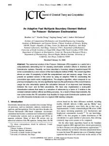
Fig. 1 BEM error for piecewise constants (p = 0) and piecewise linears (p = 1) on uniform and adaptive meshes for example (10).

O(N −1/2 )

0

10

error resp. error estimator

ηℓ =



0

10

−1

10

−2

10

O(N −3/2 ) −3

10

error, p = 0, adaptive error, p = 0, uniform estimator, p = 0, adaptive estimator, p = 0, uniform

−4

10

0

10

1

10

2

10

3

10

number of elements Fig. 2 BEM error and error estimator for piecewise constants (p = 0) on uniform and adaptive meshes for example (10).

1.3 Mathematical questions To illustrate some of the mathematical questions which have to be addressed, we consider simple toy problems for the 2D and 3D Laplacian: First, we consider the weakly singular integral equation Vφ = f

on the slit Γ = (−1, 1) × {0},

(10)

where V is the simple-layer integral operator of the 2D Laplacian (see Section 2.2 below). For given f (s, 0) = s, the unique solution of (10) is known to be p u(s, 0) = 2s/ 1 − s2 . (11) We consider BEM with piecewise constant ansatz and test functions (p = 0) as well as with discontinuous piecewise linear ansatz and test functions (p = 1). The adaptive mesh refinement is driven by some (h − h/2)-type error estimator (see Section 4.2.2 below). The initial mesh consists of one line segment of length 2.

4

M. Feischl, T. F¨uhrer, N. Heuer, M. Karkulik, D. Praetorius

initial mesh T0

T3

T6

T9

T12

Fig. 3 Sequence of adaptively generated meshes for 3D BEM with anisotropic mesh refinement for example (15).

T1

T2

T1

T

T1 T4

marked element

T3

T2

T2

isotropic refinement

vertical refinement

horizontal refinement

Fig. 4 For 3D BEM, each marked rectangle T ∈ Tℓ (left) is either refined isotropically into four elements or anisotropically into two elements.

Figs. 1 and 2 show the outcome of the numerical computations, where we compare uniform vs. adaptive meshrefinement. We plot the error (measured in the natural e −1/2 -norm) and the computed a posteriori error estimaH tor versus the number N of elements. If u was smooth, the generically optimal order of convergence would be O(N −p−3/2), see [123]. However, in the present example, the exact solution has strong (generic) singularities at the tips of the slit and thus lacks the required regularity. For uniform mesh refinement, where all line segments are bisected to obtain Tℓ+1 from Tℓ , we observe a poor convergence rate of O(N −1/2 ) for both, piecewise constants and piecewise linears, see Fig. 1. Consequently, the use of higherorder polynomials does not pay on uniform meshes. However, if we use the adaptive algorithm which automatically enforces an appropriate grading of the mesh towards the singularities of u, we observe the optimal convergence behavior O(N −3/2 ) for piecewise constants p = 0 and O(N −5/2 ) for piecewise linears p = 1. Mathematically, this observation gives rise to the following questions:

•

Does the adaptive algorithm (Algorithm 1) guarantee convergence? More precisely, is it true that ku − UℓkX → 0

as ℓ → ∞?

(12)

For uniform mesh refinement, the C´ea lemma (6) and appropriate approximation results for smooth functions guarantee that Galerkin BEM always lead to convergence Uℓ → u, independently of the overall regularity or possible singularities of the unknown solution u. As observed, this convergence can be slow. On the other hand, the adaptive algorithm

does not guarantee that the mesh-size will tend to zero as ℓ → ∞. Consequently, the convergence analysis for uniform meshes does not carry over to adaptive meshes. However, a priori arguments guarantee that nestedness Xℓ ⊆ Xℓ+1 for all ℓ ≥ 0 implies convergence of Uℓ towards some limit U∞ (see Lemma 76), but raises the important question whether we can identify u = U∞ . In particular, the numerical check for convergence will always be affirmative even if the adaptive algorithm does wrong, i.e., u 6= U∞ .

•

Empirically, the adaptive algorithm 1 does not only lead to convergence,but even ensures linear convergence, i.e., ku −Uℓ+1kX ≤ q ku −UℓkX for some uniform constant 0 < q < 1.

For some symmetric andp elliptic bilinear form b(·, ·) and the induced norm kvkX = b(v, v), the C´ea lemma (6) holds with Cell = 1 = Ccont . This implies at least ku − Uℓ+1kX ≤ ku − Uℓ kX , and the numerical experiment also shows that pre-asymptotically even q ≈ 1 can be observed, see Fig. 1.

•

Does the adaptive algorithm 1 recover the optimal rate of convergence?

Clearly, the last two questions are strongly related to the a posteriori error estimator which drives the adaptive mesh refinement. As the adaptive algorithm does not see the actual error, but only the error estimator, an a posteriori error estimator is called reliable, if it provides an upper bound for the unknown error ku − UℓkX ≤ Crel ηℓ

(13)

up to some generic constant Crel > 0. If the adaptive algorithm thus drives the error estimator to zero, this implies

Adaptive Boundary Element Methods

5

0

Mathematical details (and restrictions) for the (h − h/2)error estimator are discussed in Section 4.2.2 below.

10

error in energy norm

O(N −1/4 )

Moreover, optimal convergence behavior is also constrained by the mesh refinement used. To illustrate this, we consider the weakly singular integral equation

−1

10

uniform


V φ = f on the L-screen Γ = (−1, 1)2 \(0, 1)2 × {0},

isotropic −2

10

(15)

O(N −3/4 ) anisotropic

−3

10

1

10

2

10

3

10

4

10

5

10

number of elements Fig. 5 BEM error for piecewise constants on uniform and adaptive meshes for example (15) with isotropic and anisotropic refinement. 1

error resp. error estimator

10

0

10

−1

10

−2

10

−3

10

1

10

2

10

3

10

4

10

5

10

number of elements Fig. 6 BEM error and error estimator for piecewise constants on uniform and adaptive meshes for example (15) with isotropic and anisotropic refinement.

convergence of the overall scheme. Conversely, ηℓ is called efficient, if it provides a lower bound for the unknown error

ηℓ ≤ Ceff ku − UℓkX

(14)

up to some generic constant Ceff > 0. If ηℓ is both, efficient and reliable, the adaptive algorithm monitors the convergence behavior. Fig. 2 displays error as well as (h − h/2)-type error estimator for uniform and adaptive mesh refinement and lowestorder elements p = 0. As the curves of error and error estimator are parallel, independently of the mesh refinement, it is observed that ηℓ is reliable and efficient. The same observation is obtained for higher-order polynomials (not displayed).

•

In which situations can it be mathematically guaranteed that the BEM error is estimated reliably and efficiently?

where V now is the simple-layer integral operator of the 3D Laplacian. We consider lowest-order BEM with piecewise constant ansatz and test functions. The adaptive mesh refinement is driven by some (h − h/2)-type error estimator (see Section 4.2.2 below). The initial mesh consists of 12 uniform squares with edge length 1/2, see Fig. 3 (left). It is well-known that the solutions of (15) suffer from edge singularities. For f (x) = 1, we therefore compare uniform mesh refinement, where each square is divided into four similar squares of half edge length, with adaptive isotropic resp. anisotropic mesh refinement. In the isotropic case, marked squares are refined into four similar squares of half edge length. In the anisotropic case, we also allow that the (rectangular) elements are only refined along one edge into two rectangles, see Fig. 4. For the anisotropic refinement, some adaptively refined meshes are shown in Fig. 3. The overall outcome of these computations is visualized in Figs. 5 and 6, where we compare uniform and adaptive isotropic and anisotropic mesh refinement. We plot the e −1/2 -norm) and the comerror (measured in the natural H puted a posteriori error estimator versus the number N of elements. If u was smooth, the generically optimal order of convergence would be O(h3/2 ) for the uniform meshsize h. For 3D BEM, this corresponds to an optimal decay O(N −3/4 ) with respect to the number of elements. However, the exact solution exhibits generic singularities along the edges of Γ . For uniform mesh refinement, where all elements are refined isotropically, we observe a poor rate of convergence O(N −1/4 ) for the error. For the adaptive strategy with anisotropic elements, we observe the optimal rate of convergence O(N −3/4 ), while adaptive isotropic refinement leads to approximately O(N −1/2 ). We note that heuristic arguments show that O(N −1/2 ) is the optimal rate of convergence in the presence of generic edge singularities, if one restricts to isotropic elements [38]. This is also illustrated by the adaptive meshes shown in Fig. 7 as well as Fig. 8 which show adaptively generated anisotropic resp. isotropic meshes with (almost) the same number of elements. Fig. 6 shows the BEM error as well as the (h − h/2)-type error estimators. As for the 2D example (10), we observe that the a posteriori error estimators used are reliable and efficient.

6

M. Feischl, T. F¨uhrer, N. Heuer, M. Karkulik, D. Praetorius

defined in Section 2.6, and the resulting discrete equations are given in Section 2.7. As a basis for a posteriori error estimation, Section 3 focuses exclusively on the localization techniques for fractional order Sobolev norms. The results of this section will be used frequently in this work, and the two omnipresent approaches, localization by local fractional norms (Section 3.1) and localization by approximation (Section 3.2), will be treated in particular. Section 4 gives an overview of the different a posteriori error estimators for BEM that have been proposed in the mathematical literature. The estimators are classified into five different groups:

Fig. 7 Adaptively generated mesh with anisotropic elements.

Fig. 8 Adaptively generated mesh with isotropic elements.

1.4 Outline Essential ingredients of the mathematical theory of BEM will be collected in Section 2. The fundamental function spaces in BEM are Sobolev spaces, which will be introduced briefly in Section 2.1. There will be no further explanations on the connection of BIEs and PDEs, but in Section 2.2 we will define the boundary integral operators that constitute the equations that are to be solved (Sections 2.3 and 2.4). To emphasize the significance of local mesh refinement, Section 2.5 briefly summarizes the regularity theory in the context of this work. The terms associated with discrete spaces, such as meshes, piecewise polynomials, and so on, will be

– – – – –

Residual error estimators (Section 4.1), estimators based on space enrichment (Section 4.2), averaging on large patches (Section 4.3), ZZ-type estimators (Section 4.4), and estimators based on the Calder´on sytem (Section 4.5).

In addition, Section 4.6 deals with the question of how to estimate data approximation errors. The estimators presented up to this point might serve also in higher-order BEM, but are analyzed only with respect to mesh refinement. In contrast, a posteriori estimators and associated adaptive algorithms for p and hp-versions of the BEM are shown in Section 5. The question of convergence of h-adaptive algorithms of the type (12) will be addressed in Section 6, which deals with the so-called estimator reduction principle. This is a rather general concept dealing with convergence of adaptive algorithms. This will be explained in detail in Section 6.4. The results of Section 6 are tailored to certain concrete model problems and estimators which are given in Sections 6.5– 6.7 for a posteriori error estimation with (h − h/2), ZZ, and weighted residual estimators, as well as in Sections 6.8 and 6.9 including data approximation. We also comment on convergence in the presence of anisotropic mesh refinement in Section 6.10. The properties of module refine(·), responsible for mesh refinement, play an important role in the analysis of optimal rates of adaptive mesh-refining algorithms. Section 7 explains the requirements for refine(·) and summarizes available results from the literature to account for local refinement in 2D BEM as well as 3D BEM. Regarding the question of optimal convergence of Algorithm 1, the following Section 8 introduces an abstract framework that was recently laid out even in a more general setting in [37]. At this point, we will have fixed all the parts of Algorithm 1 except estimate . Based on certain assumptions (called (A1)–(A4)) on the estimator ηℓ that is employed in estimate , convergence of Algorithm 1 will be shown in Section 8.2, generalising the results of Section 6. Optimal convergence of Algorithm 1 within the abstract framework will be shown in Section 8.3. In

Adaptive Boundary Element Methods

Sections 8.4–8.7, it is shown how to apply the abstract setting to concrete model problems, i.e., the assumptions (A1)– (A4) will be checked for different error estimators. More precisely, we obtain linear convergence for (h − h/2)-based estimators and optimal convergence for weighted residual estimators. From Section 8.8 on, we deal with convergence and optimality of ABEM including data approximation. To that end, an extended algorithm (Algorithm 123) will be formulated that differs from Algorithm 1 only in that Galerkin solutions are computed with respect to an approximate righthand side and that error control for data approximation is included in the error estimation. For this extended error estif f A6)), mators, we again formulate assumptions (called (A1)–( and show not only convergence (Section 8.9) but also optimality (Section 8.10) of Algorithm 123. We show how to apply this abstract framework to concrete model problems in Sections 8.11 and 8.12. The final Section 9 is devoted to details in implementation. We give detailed explanations how to implement the L2 -orthogonal projection (Section 9.1) as well as the ScottZhang projection (Section 9.2). Furthermore, we show how to implement the two-level error estimator, the (h − h/2) based error estimator, as well as the weighted residual error estimator for d = 2 and in the lowest order case. The ideas that we present for implementation transfer immediately to d = 3 and higher-order polynomials. Throughout the paper, a . b means that a ≤ cb with a generic constant c > 0 that is independent of involved mesh parameters or functions. Similarly, the notation a & b and a ≃ b is used.

7

kukL p(Ω ) < ∞, where R ( Ω |u| p )1/p kukL p(Ω ) := inf M⊂Ω supx∈Ω \M |u(x)| |M|=0

hu , wiΩ :=

Z

Ω

1/2

kukL2 (Ω ) := hu , uiΩ .

uw dx,

The space C0∞ (Ω ) is the space of smooth φ ∈ C∞ (Ω ) with supp(ϕ ) ⊂ Ω . If, for u ∈ L2 (Ω ), a locally integrable function w : Ω → Rd exists such that, for all ϕ ∈ C0∞ (Ω ) Z

Ω

u(x)∇ϕ (x) dx = −

Z

For a rigorous treatise of Sobolev spaces, we refer to the standard reference [1]. For Ω ⊂ Rd an open and bounded set and p ∈ [1, ∞], L p (Ω ) denotes the space of all measurable functions u : Ω → R whose p-th power is integrable, i.e.,

Ω

w(x)ϕ (x) dx,

then w is called the weak gradient of u, abbreviated by ∇u := w. It follows from the fundamental lemma of calculus of variations that the weak gradient is uniquely defined almost everywhere, and integration by parts shows that it therefore coincides with the classical gradient of u if it exists. The space of all functions u ∈ L2 (Ω ) with weak gradient ∇u ∈ L2 (Ω ) is the Sobolev space H 1 (Ω ). This is again a Hilbert space with inner product and norm hu , wiH 1 (Ω ) := hu , wiΩ + h∇u , ∇wiΩ , 1/2

kukH 1 (Ω ) := hu , uiH 1 (Ω ) . For s ∈ (0, 1), the fractional order Sobolev space H s (Ω ) consists of all u ∈ L2 (Ω ) with kukH s (Ω ) < ∞, where inner product and norm are

+

2 Mathematical foundation of the BEM

2.1 Sobolev spaces

for p = ∞.

The space L2 (Ω ) is a Hilbert space with inner product and norm

hu , wiH s (Ω ) := hu , wiΩ

This section briefly introduces the mathematical framework for boundary element methods. Definitive books in this respect are [98,108,114], which deal exclusively with boundary integral equations and their analytical underpinning, and [123,135], which focus to a great extent on boundary element discretizations. Let us also note that the analysis of finite elements for the discretization of boundary integral equations of the first kind goes back to N´ed´elec and Planchard [115], and Hsiao and Wendland [97].

for p < ∞,

Z Z

Ω Ω

(u(x) − u(y))(w(x) − w(y))

1/2

|x − y|d+2s

dx dy,

kukH s (Ω ) := hu , uiH s (Ω ) . Generally, for a non-empty set ω ⊂ Ω and s ∈ (0, 1), the associated seminorm is denoted by |u|2H s (ω ) :=

Z Z

ω ω

(u(x) − u(y))2 |x − y|d+2s

dx dy.

From now on we assume that Ω is simply connected and has a Lipschitz boundary ∂ Ω , i.e., local orthogonal coordinates may be introduced to represent ∂ Ω locally as a Lipschitz function over a (d − 1)-dimensional domain. Then, we can define Sobolev spaces H s (Γ ) for Γ ⊆ ∂ Ω and associated inner products and norms for s ∈ [0, 1) exactly as for (d − 1)-dimensional domains but using surface integrals instead of integrals over domains. The definition of the surface integral does not depend on the parametrization used, so neither does the space H s (Γ ) and its inner product or norm for s ∈ [0, 1). Independently of the chosen parametrization

8

M. Feischl, T. F¨uhrer, N. Heuer, M. Karkulik, D. Praetorius

of Γ , a weak surface gradient ∇Γ can be defined, cf. [144, Def. 1.9] or [47, Appendix A.3], and hence a space H 1 (Γ ). The surface gradient is tangential to Γ , and for smooth functions u in Rd there holds ∇u = ∇Γ u + (n · ∇u) · n. For d = 2, i.e., Γ a one-dimensional curve, the notation u′ will be used to denote the gradient of u. For s ∈ [0, 1], define  e s (Γ ) := u ∈ H s (∂ Ω ) | supp(u) ⊂ Γ H with norm

kukHes (Γ ) := ke ukH s (∂ Ω ) ,

(16)

where ue denotes the extension of u by zero on ∂ Ω . Clearly, if Γ = ∂ Ω is the boundary of a bounded Lipschitz domain, it e s (Γ ) = H s (Γ ) for all s ∈ [0, 1]. The same space holds that H can be defined for a domain Ω instead of Γ by using Rd instead of ∂ Ω . A different characterization of the spaces e s (Ω ) can be given; to that end, we introduce the trace opH erator γ0 , which is defined for smooth functions u as γ0 u := u|∂ Ω . It can be shown that kγ0 ukH s−1/2 (∂ Ω ) ≤ Cs kukH s (Ω ) for s ∈ (1/2, 1], hence γ0 can be extended to a linear and continuous operator from H s (Ω ) to H s−1/2 (Γ ) for s ∈ (1/2, 1]. It is known that e s (Ω ) = {u ∈ H s (Ω ) | γ0 u = 0} H e s (Ω ) = H s (Ω ) H

for s ∈ (1/2, 1], for s ∈ [0, 1/2).

e s (Ω ) from (16) Furthermore, in these cases, the norms on H s and the norms on H (Ω ) are equivalent, and the equivalence constants depend on s and Ω , cf. [80, Lem. 1.3.2.6 and Thm. 1.4.4.4]. If s ∈ {0, 1}, the norms coincide. Note that the case s = 1/2 is excluded. Likewise, an operator γ1 can be defined which extends the (co-)normal derivative. For a linear operator B : X → Y between two normed linear spaces, denote its operator norm by kBkX →Y := sup

06=x∈X

kB(x)kY . kxkX

The operator B is called bounded if kBkX →Y < ∞. The dual space of a normed linear space X , denoted by X ′ , consists of all linear and bounded operators (so-called functionals) f : X → R. A norm on X ′ is given by k f kX ′

| f (x)| := k f kX →R = sup . kxk X 06=x∈X

For the Sobolev space H s (Γ ), the dual space can be characterized by the concept of the so-called Gelfand triple, cf. [123, Sec. 2.1.2.4], using the fact that for densely embedded Hilbert spaces V ⊂ U , their dual spaces are also densely embedded, i.e., U ′ ⊂ V ′ . Then, identifying U with its dual U ′ , the scalar product h· , ·iU can be extended to a duality pairing between V and its dual V ′ . The space U

is called pivot space. The described concept is used to define the duality pairing between H s (Γ ) for s > 0 and its dual e −s (Γ ) := H s (Γ )′ , where L2 (Γ ) is used as pivot space. The H e −s (Γ ) are both in consequence is that, if u ∈ H s (Γ ) and v ∈ H L2 (Γ ), then hu , viH s (Γ )×He−s (Γ ) = hu , viΓ coincides with the L2 (Γ ) scalar product, and the last expression will be used from now on to denote the duality pairing. The dual space e s (Γ ) for s > 0 will be denoted by H −s (Γ ). of H Certain equations that will be considered have a kernel, hence a quotient space will be needed to solve them. For s ∈ [−1, 1], define H0s (Γ ) := {u ∈ H s (Γ ) | hu , 1iΓ = 0} .

Remark 1 In the literature, cf. [123,135], Sobolev spaces are defined with a fixed parametrization and associated partition of unity on Γ . This gives an equivalent definition to ours, with constants that depend on the chosen parametrization. To see this, denote by a a specific parametrization and partition of unity on Γ , and associated norms k · ks,a . It follows immediately that k · ks,a ≤ Ca k · kH s (Γ ) , and the reverse inequality can be proven with the same arguments as in the proof of Theorem 17 below.

2.2 Boundary integral operators From now on, Ω ⊂ Rd will always denote a bounded, simply connected, d-dimensional domain with Lipschitz boundary ∂ Ω and outer normal vector n(y) for y ∈ ∂ Ω , and Γ will denote a (d − 1)-dimensional subset Γ ⊂ ∂ Ω . For simplicity, in the case d = 2, we assume that cap(∂ Ω ) < 1, see [108], which can always be fulfilled by scaling Ω such that its diameter is smaller than 1. In order to transform a given PDE into an equivalent boundary integral equation, a fundamental solution of the PDE at hand needs to be available. For the Laplace operator −∆ , the fundamental solution is given by ( for d = 2, − 1 log |z| G(z) := 1 2π1 for d = 3. 4π |z| For densities φ , v : Γ → R and x ∈ Rd \ Γ , define the following potentials: – the single layer potential of φ as Ve φ (x) :=

Z

Γ

G(x − y)φ (y) d Γ (y),

– and the double layer potential of v as e Kv(x) :=

Z

Γ

∂n(y) G(x − y)v(y) dΓ (y).

Adaptive Boundary Element Methods

9

At least for φ , v ∈ L1 (Γ ), these operators are smooth away e ∈ C∞ (Rd \ Γ ), and also harmonic, i.e., from Γ , i.e., Ve φ , Kv e e ∆ V φ = 0 = ∆ Kv on Rd \ Γ . Starting from these definitions, boundary integral operators are defined as e, V := γ0V

e K := 1/2 + γ0K,

e W := −γ1 K,

K ′ := −1/2 + γ1Ve .

The operator V is called the single layer operator, W the hypersingular operator, and K and K ′ the double layer operator and its adjoint, respectively. The two following results recall the stability and ellipticity properties of these boundary integral operators. For proofs and further references, we refer to [49,108,123,144]. Theorem 2 For Γ = ∂ Ω a Lipschitz boundary and s ∈ [−1/2, 1/2], the boundary integral operators are bounded as mappings V : H −1/2+s(Γ ) → H 1/2+s (Γ ) K ′ : H −1/2+s(Γ ) → H −1/2+s(Γ ) W :H

(Γ ) → H

−1/2+s

If Γ ⊂ ∂ Ω , ∂ Ω again a Lipschitz boundary, it holds e −1/2+s(Γ ) → H 1/2+s (Γ ) V :H

Proposition 6 (Hypersingular integral equation) Denote by Ω ⊂ Rd a Lipschitz domain and Γ ( ∂ Ω a simply connected, open surface. Given φ ∈ H −1/2 (Γ ), there is a unique e 1/2 (Γ ) of the variational problem solution u ∈ H e 1/2 (Γ ). for all v ∈ H

hWu , viΓ + hu , 1iΓ hv , 1iΓ = hφ , viΓ u

for all φ ∈ H −1/2(Γ ),

hWu , uiΓ + hu , 1iΓ2 ≥ Cell kuk2H 1/2 (Γ )

for all u ∈ H 1/2 (Γ ).

If Γ ( ∂ Ω is only a subset, then there holds e −1/2 (Γ ), for all φ ∈ H

e 1/2 (Γ ). for all u ∈ H

The constant Cell depends only on Γ .

2.3 Weakly singular integral equations According to Theorems 2 and 3, hV · , ·iΓ is a scalar prode −1/2(Γ ), such that the Riesz representation theuct on H orem immediately yields solutions to the following variational formulations. Proposition 4 (Weakly singular integral equation) Denote by Ω ⊂ Rd a Lipschitz domain with cap(∂ Ω ) < 1 for d = 2 and Γ ⊂ ∂ Ω . Given f ∈ H 1/2 (Γ ), there is a unique solution e −1/2(Γ ) of the variational problem φ ∈H hV φ , ψ iΓ = h f , ψ iΓ

Likewise, Theorems 2 and 3 state that hW · , ·iΓ is a scalar e 1/2 (Γ ) if Γ ( ∂ Ω is an open surface, while product on H hW · , ·iΓ + h· , 1iΓ h· , 1iΓ is a scalar product on H 1/2 (Γ ) in case of Γ = ∂ Ω .

−1/2

Theorem 3 If Γ = ∂ Ω is the boundary of a Lipschitz domain Ω , then there holds ellipticity

hWu , uiΓ ≥ Cell kuk2He 1/2 (Γ )

2.4 Hypersingular integral equations

Provided that φ ∈ H0

e 1/2+s (Γ ) → H −1/2+s (Γ ). W :H

hV φ , φ iΓ ≥ Cell kφ k2H −1/2 (Γ )

for all ψ ∈ H −1/2 (Γ ).

If Γ = ∂ Ω , then there is a unique solution u ∈ H 1/2 (Γ ) of the variational problem

(Γ ).

hV φ , φ iΓ ≥ Cell kφ k2He−1/2 (Γ )

hV φ , ψ iΓ = h(1/2 + K) f , ψ iΓ

hWu , viΓ = hφ , viΓ

K : H 1/2+s(Γ ) → H 1/2+s (Γ ) 1/2+s

Proposition 5 (Dirichlet problem) Denote by Ω ⊂ Rd a Lipschitz domain with cap(∂ Ω ) < 1 for d = 2 and Γ = ∂ Ω . Given f ∈ H 1/2 (Γ ), there is a unique solution φ ∈ H −1/2 (Γ ) of the variational problem

e −1/2 (Γ ). for all ψ ∈ H

for all v ∈ H 1/2 (Γ ).

(Γ ), the solution satisfies

1/2 ∈ H0 (Γ ).

Proposition 7 (Neumann problem) Denote by Ω ⊂ Rd a −1/2 Lipschitz domain and Γ = ∂ Ω Given φ ∈ H0 (Γ ), there 1/2

is a unique solution u ∈ H0 (Γ ) of the variational problem hWu , viΓ + hu , 1iΓ hv , 1iΓ = h(1/2 − K ′)φ , viΓ

for all v ∈ H 1/2 (Γ ).

2.5 Regularity of solutions It is well known that solutions to BVPs10 on non-smooth domains have in general limited regularity, even for smooth data. For polygonal/polyhedral domains and standard elliptic operators of second order there exists a precise regularity theory that proves that this regularity reduction is due to the presence of so-called corner singularities (on polygons and polyhedra) and corner-edge singularities (on polyhedra). In this paper we are studying the solution of integral equations of the first kind where unknowns are Cauchy data of BVP. Therefore, through trace operations (extended restriction and normal derivative), singular behavior of solutions to BVP imply in a natural way singular behavior of solutions to such integral equations. 10

boundary value problem (BVP)

10

M. Feischl, T. F¨uhrer, N. Heuer, M. Karkulik, D. Praetorius

For an overview of regularity theory for BVP on nonsmooth domains we refer to the monograph by Dauge [53]. The singularity expressions by Dauge have been extensively studied by Stephan and von Petersdorff [146,147,148]. Their main contribution is tensor product expansions of singularities so that they are accessible to approximation analysis by piecewise polynomial functions. In this way, precise predictions can be made about convergence orders of FE and BE approximations. In two dimensions, the study of corner singularities goes back to the seminal paper by Kondratiev [104] and, of course, the structure of the appearing singularities is much simpler. We note that for an optimal error analysis of hp-methods with geometric mesh refinement, a more specific regularity analysis based on countably normed weighted spaces is in order. We refer to [95,96] for a corresponding regularity theory of boundary integral equations on polygons. To our knowledge [106], Maischak and Stephan have a manuscript analyzing the case of the hypersingular integral equation (governing the Laplacian) on polyhedral surfaces. Low-order methods severely suffer from the presence of singularities. They limit the order of convergence of the boundary element method when quasi-uniform meshes are used. Adaptive methods refine meshes locally by using information that stems from a posteriori error estimation. In this way, adaptivity aims at recovering the orders of convergence that one would obtain for smooth solutions and quasiuniform meshes. In the following, for some typical cases, we recall what are the principal singularities that one has to expect in solutions to the hypersingular and weakly singular boundary integral equations. These results stem from the previously mentioned publications [104,53,147,148].

Two space dimensions. Let Γ be the boundary of a simply connected polygon with edges Γ j , vertices t j and angles ω j at the vertices ( j = 1, . . . , J). We consider the weakly singular integral equation from Proposition 4 (with solution φ and right-hand side function f ) and the hypersingular integral equation from Proposition 6 (with solution u and right-hand side function g). For piecewise analytic data f , g, the solutions φ and u behave singularly at the corners of the polygon and are smooth elsewhere. To be precise we consider a partition of unity (χ1 , . . . , χJ ) where χ j is the restriction of a C0∞ (R2 ) function to Γ such that χ j = 1 in a neighborhood of the vertex t j and supp(χ j ) ⊂ Γ j−1 ∪ {t j } ∪ Γ j (Γ 0 = Γ J ). In this way we may write any function ϕ on Γ like

ϕ=

J

∑ (ϕ− , ϕ+ )χ j

j=1

where a pair (ϕ− , ϕ+ ) corresponds to ϕ on Γ j−1 ∪ {t j } ∪ Γ j with

ϕ− = ϕ |Γ j−1

and ϕ+ = ϕ |Γ j .

From [50,94] we cite the following result. Let α jk := k ωπj (integer k ≥ 1, j = 1, . . . , J) and, for t ≥ ω

1/2, let n be an integer with n + 1 > πj (t − 1/2) ≥ n. (i) If f is a piecewise analytic function, then there exists a function φ0 with φ0 |Γ j ∈ H t−1 (Γ j ) such that, for the solution φ of the weakly singular integral equation, there holds

φ=

J

n

∑∑

j=1 k=1


(φ jk )− , (φ jk )+ χ j + φ0 .

Here, (φ jk )± (x) = c|x − t j |α jk −1 if α jk is not an integer and (φ jk )± (x) = c1 |x − t j |α jk −1 + c2 |x − t j |α jk −1 log |x − t j | if α jk is an integer. (ii) If g is a piecewise analytic function, then there exists a function u0 with u0 |Γ j ∈ H t (Γ j ) such that, for the solution u of the hypersingular integral equation, there holds J

u=

n

∑∑

j=1 k=1


(u jk )− , (u jk )+ χ j + u0.

Here, (u jk )± (x) = c|x − t j |α jk if α jk is not an integer and (u jk )± (x) = c1 |x − t j |α jk + c2 |x − t j |α jk log |x − t j | if α jk is an integer. The constants c, c1 and c2 above (in (i) and (ii)) are generic. The representation of singularities above is valid also in the case of open curves, by setting the angles ω j = 2π at the endpoints. For example, Γ being an interval in R2 , the solution φ of the weakly singular integral equation has (with t0 being any endpoint of Γ ) singularities of the form

φ (x) ∼ |t0 − x|−1/2

(x close to t0 )

and the solution u of the hypersingular integral equation behaves like u(x) ∼ |t0 − x|1/2

(x close to t0 ).

An illustration of both cases is given in Figures 9, 10. Concluding, the solutions of the integral equations are smooth away from the corners and have reduced regularity at the corners. In the case of the weakly singular equation,

Adaptive Boundary Element Methods

11

(ii) The edge singularities φ e , ue have the form  e 

φe =

ue =

me

sj

j=1

s=0

me

Three space dimensions. For simplicity we restrict our presentation of singularities in three dimensions to the case of Γ being a plane open surface with polygonal boundary. We use the results from [147,148] and follow the notation from [22,25], see also [127]. Again, we consider the weakly singular integral equation from Proposition 4 (with solution φ and right-hand side function f ) and the hypersingular integral equation from Proposition 6 (with solution u and right-hand side function g). As before, we assume that f and g are sufficiently smooth. In the following we present the singularities of φ and u together. Let V and E denote the sets of vertices and edges of Γ , respectively. For v ∈ V , let E(v) denote the set of edges with v as an endpoint. Then, φ and u are of the form

φ = φreg + ∑ φ e + ∑ φ v + ∑

∑

φ ev ,

u = ureg + ∑ u + ∑ u + ∑

∑

uev ,

e∈E

v∈V

e

e∈E

v nv qi

λ v −1 v wit (θv ),

i=1 t=0 v nv qi

λv

u = χ (rv ) ∑ ∑ Bvit | log rv |t rv i wvit (θv ), v

i=1 t=0

v ≥ λ v > 0, n , qv ≥ 0 are integers, and Bv are real where λi+1 v i i it numbers. Here, χ v is a C∞ cut-off function with χ v = 1 for 0 ≤ rv ≤ τv and χ v = 0 for rv ≥ 2τv with some τv ∈ (0, 12 ). The functions wvit are in H q (0, ωv ) for q as large as required. Here, ωv denotes the interior angle (on Γ ) between the edges meeting at v. (iv) The edge-vertex singularities φ ev , uev have the form

φ ev = φ1ev + φ2ev ,

ev uev = uev 1 + u2 ,

where

φ1ev =

me nv



sej qvi



s

∑ ∑  ∑ ∑ ∑ Bevijlts | log xe1 |s+t−l | log xe2 |l 

j=1 i=1

s=0 t=0 l=0

λ v −γ ej γ ej −1 v xe2 χ (rv )χ ev (θv ),

xe1i

uev 1 =

me nv



sej qvi



s

∑ ∑  ∑ ∑ ∑ Bevijlts | log xe1 |s+t−l | log xe2 |l 

j=1 i=1

s=0 t=0 l=0

λ v −γ ej γ ej v xe2 χ (rv )χ ev (θv )

xe1i

and

v∈V e∈E(v)

where, using local polar and Cartesian coordinate systems (rv , θv ) and (xe1 , xe2 ) with origin v, there hold the following representations: (i) The regular parts satisfy φreg ∈ H k (Γ ), ureg ∈ H k+1 (Γ ), with k > 0.

γe

φ = χ (rv ) ∑ ∑ Bvit | log rv |t rv i

v∈V e∈E(v)

v

v∈V

s=0

v

v

the solution can be unbounded at corners and in the case of the hypersingular equation, gradients (derivatives with respect to the arc-length) can be unbounded there. In the extreme case of an open polygon, the singularity | · −t0 |−1/2 prevents φ from being an L2 (Γ )-function and, similarly, u with its | · −t0|1/2 -singularity is not an element of H 1 (Γ ).



sej

where γ ej+1 ≥ γ ej ≥ 21 , and me , sej are integers. Here, χ1e , χ2e are C∞ cut-off functions with χ1e = 1 in a certain distance to the endpoints of e, and χ1e = 0 in a neighbourhood of these vertices. Moreover, χ2e = 1 for 0 ≤ xe2 ≤ δe and χ2e = 0 for xe2 ≥ 2δe with some δe ∈ (0, 12 ). The functions bejs χ1e are in H m (e) for m as large as required. (iii) The vertex singularities φ v , uv have the form v

Fig. 10 Typical singular solution of the hypersingular integral equation on an interval



χ1e (xe1 )χ2e (xe2 ),

∑  ∑ bejs(xe1 )| log xe2 |s  xe2j χ1e (xe1 )χ2e (xe2 ),

j=1

Fig. 9 Typical singular solution of the weakly singular integral equation on an interval

γ e −1

∑  ∑ bejs(xe1 )| log xe2 |s  xe2j

φ2ev

e me s j

=

γ e −1

∑ ∑ Bevjs (rv )| log xe2 |s xe2j

χ v (rv )χ ev (θv ),

j=1 s=0

uev 2

e me s j

=

γe

∑ ∑ Bevjs (rv )| log xe2 |s xe2j χ v (rv )χ ev (θv ),

j=1 s=0

12

M. Feischl, T. F¨uhrer, N. Heuer, M. Karkulik, D. Praetorius

Fig. 11 Typical singular solution of the weakly singular integral equation on the open surface (0, 1) × (0, 1) × {0}

Fig. 12 Typical singular solution of the hypersingular integral equation on the open surface (0, 1) × (0, 1) × {0}

with

of piecewise polynomials over a mesh of Γ . The related terms will be introduced in this section.

Bev js (rv ) =

s

∑ Bevjsl (rv )| log rv |l .

l=0

Here, qvi , sej , λiv , γ ej , χ v are as above, Bev i jlts are real numbers, and χ ev is a C∞ cut-off function with χ ev = 1 for 0 ≤ θv ≤ βv and χ ev = 0 for 23 βv ≤ θv ≤ ωv for some βv ∈ (0, min{ωv /2, π /8}]. The functions Bev jsl may be chosen such that v ev e Bev js (rv ) χ (rv )χ (θv ) = χ js (xe1 , xe2 ) χ2 (xe2 ),

where the extension of χ js by zero onto R2+ := {(xe1 , xe2 ); xe2 > 0}

lies in H m (R2+ ) for m as large as required. Here, χ2e is a C∞ cut-off function as in (ii). Concluding, on open surfaces, both integral equations have solutions with singularities. The strongest ones are of the edge-type dist(·, ∂Γ )−1/2 for the solution φ of the weakly singular equation. In this case, φ is not an element of L2 (Γ ), as in the case of two dimensions on open curves. Correspondingly, the strongest singularities of the solution u of the hypersingular equation are of the type dist(·, ∂Γ )1/2 so that u 6∈ H 1 (Γ ), again analogously to the case in two dimensions. In Figures 11, 12 we present typical solutions to both integral equations on the open surface Γ = (0, 1) × (0, 1) × {0}. It remains to mention that on polyhedral surfaces, singularities have the same structure but with larger exponents defining the edge and edge-vertex singularities, cf. [147,148] for more details.

2.6 Discrete spaces The discrete spaces that will be used to approximate the solutions of the problems given by Propositions 4–7 are spaces

2.6.1 Meshes Definition 8 A mesh T on Γ ⊂ ∂ Ω is a finite, mutually disjoint partition T = {T1 , . . . , TM } with the following properties: – every element T ∈ T is a d-simplex, i.e., the interior of the convex hull of d points x1 , . . . , xd , S – Γ= M i=1 T i , ′ – the intersection T ∩ T is either empty, a common point, or a common edge of both T and T ′ . The collection of all points N := {x1 , . . . , xN } that constitute the elements is called the set of nodes of T . Associated to a mesh T is the local mesh-width function hT ∈ L∞ (Γ ), given T -element-wise as hT |T := hT (T ) := |T |1/(d−1). On certain occasions the index T will be omitted if no confusion can arise, i.e., hT will be used instead of hT |T . The quantity

σT :=

   

diam(T ) diam(T ′ ) ′ T,T ′ ∈T ,T ∩T 6=0/ sup

d−1   max diam(T ) |T | T ∈T

for d = 2, for d ≥ 3,

is usually called the shape-regularity constant of T , and it is a measure for the degeneracy of the elements T . Remark 2 To say that a constant C in a statement depends on shape-regularity means that, given some constant σ > 0, there is a constant C(σ ), depending only on σ , such that the statement holds true for all meshes T as long as σT ≤ σ .

Adaptive Boundary Element Methods

13

For a node z ∈ N , the node-patch ωz is the collection of all elements T ∈ T which share z, same idea for the elementpatch ωT , i.e.,  ωz := T ∈ T | z ∈ T  ωT := T ′ ∈ T | T ′ ∩ T 6= 0/ .

An important concept is the so-called reference element Tref , which is chosen to be fixed throughout, e.g., as the interior of the convex hull of (0, 0), (1, 0), and (0, 1). Every element T ∈ T with nodes {x0 , x1 , x2 } is then the image T = FT (Tref ) of Tref under the affine mapping ( R2 → R3 FT : x 7→ BT x + x0 , with matrix BT = (x1 − x0 | x2 − x0 ) ∈ R3×2 . 2.6.2 Polynomial spaces

hV Φ , Ψ iΓ = h(1/2 + K) f , Ψ iΓ

polynomial spaces on a mesh T are defined by

P (T ) := {u ∈ L∞ (Γ ) | u ◦ FT ∈ P (Tref ) for all T ∈ T } p

p

S p (T ) := P p (T ) ∩C0 (Γ ).

For Γ ( ∂ Ω , define the space with vanishing boundary conditions fp (T ) := H e 1/2 (Γ ) ∩ S p (T ). S Remark 3 If a mesh carries an index, e.g., Tℓ , it’s associated quantities are also equipped with this index, e.g., σℓ denotes the shape-regularity constant, hℓ the mesh-width, Nℓ the set of nodes, and so on.

2.7 Galerkin formulation Discrete approximations to the exact solutions φ and u of the Problems in Propositions 4–7 can be computed by change ±1/2 (Γ ) to the discrete ing the infinite dimensional spaces H p p spaces P (T ) and S (T ). The fact that we can also use functions of the discrete spaces in the variational formulations provides best-approximation estimates (C´ea’s Lemma). Proposition 9 (Galerkin for weakly singular) There is a unique solution Φ ∈ P p (T ) of for all Ψ ∈ P p (T ).

for all Ψ ∈ P p (T ).

e −1/2 (Γ ) is the solution of Proposition 4 Lemma 11 If φ ∈ H or Proposition 5, and Φ ∈ P p (T ) is the solution of Proposition 9 or 10, then kφ − Φ kHe−1/2 (Γ ) ≤

Ccont min kφ − Ψ kHe−1/2 (Γ ) . Cell Ψ ∈P p (T )

Here, Ccont = kV kHe−1/2 (Γ )→H 1/2 (Γ ) is the stability constant of V , cf. Theorem 2, and Cell is its ellipticity constant, cf. Theorem 3.

Proposition 12 (Galerkin for hypersingular) In the case Γ ( ∂ Ω , there is a unique solution U ∈ Sfp (T ) of hWU ,V iΓ = hφ ,V iΓ

Denoting for p ≥ 0 the polynomial space on the reference element by n o P p (Tref ) := span (x, y) ∈ R2 7→ xi yk | 0 ≤ i + k ≤ p ,

hV Φ , Ψ iΓ = h f , Ψ iΓ

Proposition 10 (Galerkin for Dirichlet) There is a unique solution Φ ∈ P p (T ) of

fp (T ). for all V ∈ S

In the case Γ = ∂ Ω , there is a unique solution U ∈ S p (T ) such that for all V ∈ S p (T ) hWU ,V iΓ + hU , 1iΓ hV , 1iΓ = hφ ,V iΓ . −1/2

If φ ∈ H0

(Γ ), it holds that hU , 1iΓ = 0.

Proposition 13 (Galerkin for Neumann) There is a unique solution U ∈ S p (T ) such that for all V ∈ S p (T ) hWU ,V iΓ + hU , 1iΓ hV , 1iΓ = h(1/2 − K ′)φ ,V iΓ . e 1/2 (Γ ) is the solution of Proposition 6 Lemma 14 If u ∈ H fp (T ) resp. U ∈ S p (T ) is the or Proposition 7, and U ∈ S solution of Proposition 12 or 13, then ku − UkHe1/2(Γ ) ≤

Ccont min ku − VkHe1/2 (Γ ) . Cell V ∈S p (T )

Here, Ccont = kW kHe1/2 (Γ )→H −1/2 (Γ ) is the stability constant of W , cf. Theorem 2, and Cell is its ellipticity constant, cf. Theorem 3.

Note that the discrete formulations of Propositions 9– 13 are, indeed, linear systems of equations. A distinct feature of boundary element methods is that, due to the non-locality of the boundary integral operators, the system matrices are dense, and therefore sophisticated data compression techniques are used to reduce complexity for assembling and solving. In Propositions 10 and 13, also the right-hand sides contain boundary integral operators. There are fast methods to compute the right-hand sides, cf. [48,126], but if one wants to re-use the fast method that is employed for system matrices, the data f resp. φ needs to be approximated by discrete functions.

14

M. Feischl, T. F¨uhrer, N. Heuer, M. Karkulik, D. Praetorius

Proposition 15 (Galerkin for Dirichlet with data approximation) Denote by JT : H 1/2 (Γ ) → S p+1 (T ) a H 1/2 (Γ ) stable projection. Then, there is a unique solution Φ ∈ P p (T ) of

Proof In the following, we use the abbreviation

hV Φ , Ψ iΓ = h(1/2 + K)JT f , Ψ iΓ

The idea of the proof is to write

for all Ψ ∈ P p (T ).

Proposition 16 (Galerkin for Neumann with data approximation) Denote by πTp−1 : L2 (Γ ) → P p−1(T ) the L2 (Γ )orthogonal projection. Then, there is a unique solution U ∈ S p (T ) such that for all V ∈ S p (T ) hWU ,V iΓ + hU , 1iΓ hV , 1iΓ = h(1/2 − K ′)πTp−1 φ ,V iΓ .

Z Z Y

:=

Z Z Y

X

|v|2H s (Γ ) =

≃

∑

T ∈T

(17)

The spaces and dual spaces that are used in the variational formulations of integral equations are usually equipped with non-local norms. For example, the residual V Φ − f of a weakly singular integral equation is computable but has to be measured in the non-local norm of the space H 1/2 (Γ ). However, only the knowledge of the residuals local contributions enables us to define local error indicators that can be used for local mesh refinement in adaptive algorithms. Different possibilities to localize a non-local norm are available and will be presented in this section.

3.1 Localization by local fractional order norms In general, (17) does not hold equivalently with constants that are independent of the mesh T . Fortunately, this is no longer true if additional properties of the functions under consideration are assumed. The following result is shown in [63] for d = 2 and in [64] for d = 3. Theorem 17 If T is a mesh on Γ and s ∈ (0, 1), then it holds for all v ∈ H s (Γ ) that |v|2H s (Γ ) ≤

∑

z∈N

|v|2H s (ωz ) + Cloc

∑

T ∈T

2 h−2s T kvkL2 (T ) ,

where Cloc depends only on s and Γ .

∑

|x − y|d−1+2s

Z Z

ωT

T

(18)

∑

+

T ∈T

dx dy.

Z Z

(19)

T Γ \ωT

and bound the second term via the triangle inequality Z Z

T Γ \ωT

.

Z

T

Z

|v(y)|2

Z

Γ \ωT

|v(x)|2

Γ \ωT

The numerical analysis of boundary element methods takes place in the Sobolev spaces H s (Γ ) for s ∈ [−1, 1] that are defined in Section 2. Apart from the exceptional cases H 0 (Γ ) = L2 (Γ ) and H 1 (Γ ), all other spaces are equipped with norms that are either non-local (s ∈ (0, 1)) or additionally impossible to compute (s ∈ [−1, 0)). A norm is understood to be non-local if it is not possible to split its square into contributions on the elements of a mesh, i.e., if one cannot write kuk2H s (T ) .

X

T ∈T

3 Localization of fractional order Sobolev norms

kuk2H s (Γ )

|v(x) − v(y)|2

Z

T

|x − y|−d+1−2s dx dy + |x − y|−d+1−2s dx dy.

One shows that the sum over all T ∈ T of the second part on the right-hand side is the same as the sum over the first part, hence

∑

T ∈T

Z Z

T Γ \ωT

.

∑

T ∈T

Z

T

|v(y)|2

Z

Γ \ωT

|x − y|−d+1−2s dx dy.

Finally, direct calculation for d = 2 and the use of polar coordinates for d = 3 shows Z

Γ \ωT

|x − y|−d+1−2s dx . h−2s T .

The first term on the right-hand side of (19) can be estimated immediately via

∑

T ∈T

Z Z T

ωT

≤

∑

z∈N

|v|2H s (ωz ) , ⊓ ⊔

which finishes the proof.

The estimate (18) already provides a reliable localization of the non-local H s -norm, independent of the shape-regularity of the mesh. However, choosing v constant on Γ shows that the reverse inequality to (18) cannot hold in general, i.e., the bound (18) is not efficient. However, efficiency can be shown to hold when certain orthogonality is available. More precisely, the following estimate from [64, Lemma 3.4] enables us to bound the L2 -terms on the right-hand side of (18) by local H s -terms. The benefit will be twofold: First, it will enable us to show efficiency of the localization (18) on shaperegular meshes. Second, it provides us with another localization which is always efficient as well as reliable on shaperegular meshes (Theorem 19). Lemma 18 Let ω ⊆ Γ be a measurable set, s ∈ (0, 1), and u ∈ H s (ω ). Then, kuk2L2(ω ) ≤

diam(ω )d−1+2s 2 1 |u|H s (ω ) + 2 |ω | |ω |

Z

ω

u(x) dx

2

.

Adaptive Boundary Element Methods

15

In particular, if T is a mesh on Γ and hu , ΨT iΓ = 0 for ΨT ∈ P 0 (T ) the characteristic function of an element T ∈T, kuk2L2 (T ) ≤

σT h2s T |u|2H s (T ) . 2

(20)

If hu , Ψz iΓ = 0 for Ψz ∈ S 1 (T ) the hat-function function of a node z ∈ N , kuk2L2 (ωz ) ≤ C

diam(ωz )d−1+2s 2 |u|H s (ωz ) , |ω z |

(21)

where the constant C > 0 depends only on d. Proof To see the first estimate, note that 2 |ω | kuk2L2(ω ) = =

Z Z

ω ω

Z Z

|u(x)|2 dx dy +

Z Z

ω ω

|u(y)|2 dx dy

|u(x) − u(y)|2 dx dy Z 2 +2 u(x) dx .

ω ω

ω

Since for all x, y ∈ ω with x 6= y it holds 1

1 ≤ diam(ω )

d−1+2s

|x − y|d−1+2s

,

the first estimate follows. To show (20), choose ω = T and observe that diam(T )d−1+2s 2 |T |

≤

hu , ΨT iΓ =

σT h2s T Z

2

and

u(x) dx = 0.

T

To show (21) note first that Z

ωz

u Ψz dx = 0

for all z ∈ NT ,

where Ψz is the T -piecewise linear and continuous basis function for z. The Cauchy-Schwarz inequality shows Z Z u dx = (1 − Ψz)u dx ≤ k1 − ΨzkL (ω ) kukL (ω ) . 2 z 2 z ωz

ωz

A direct calculation shows that ( |ωz | /2 for d = 3, 2 k1 − ΨzkL2 (ωz ) = |ωz | /3 for d = 2,

hence Z u dx ≤ q |ωz |1/2 kukL (ω ) , 2 z ωz

for some q < 1 depending only on d. This concludes (21). ⊓ ⊔

The two preceding results show that the localization (18) is always reliable and, on shape-regular meshes, also efficient. We can combine the results also to obtain a localization which is always efficient, and, on shape-regular meshes also reliable. Theorem 19 Denote by T a mesh on Γ and let s ∈ (0, 1). Suppose that XT is a discrete space with P p (T ) ⊆ XT or R S p (T ) ⊆ XT . Then for all v ∈ H s (Γ ) with Γ vΨ dx = 0 for all Ψ ∈ XT , it holds that kvk2H s (Γ ) ≃

∑

z∈N

|v|2H s (ωz ) .

(22)

The constant in the lower bound depends only on s and Γ , while the constant in the upper bound additionally depends on shape-regularity. Proof The lower bound & follows immediately from the definition of the norms and the fact that every T ∈ T is part of at most d node-patches ωz . Now, we show the upper bound if P p (T ) ⊆ XT . Since P 0 (T ) ⊆ P p (T ), the estimate (20) can be used in (18) to show |u|2H s (Γ ) ≤

∑

z∈N

|u|2H s (ωz ) + Cloc

σT 2

∑

T ∈T

|u|2H s (T ) ,

s s s s and furthermore, due to h2s T ≤ σT |T | ≤ σT |Γ | ,

kuk2L2(Γ ) ≤

σT1+s |Γ |s ∑ |u|2H s (T ) . 2 T ∈T

Using again the fact that every element T ∈ T it part of at most d patches ωz finally shows the upper bound in (22). Suppose now that S p (T ) ⊆ XT . Since 1 S (T ) ⊆ S p (T ), the upper bound follows from the same arguments as in the case P p (T ) ⊆ XT , using (21) instead of (20). ⊓ ⊔ The sets to which the norm on the left-hand side of (18) is localized are overlapping. This overlap can be omitted if further assumptions on u are imposed. The proof of the next Lemma first appeared in [146, Lemma 3.2] if norms are defined by a method called complex interpolation, and in [2, Thm. 4.1] if norms are defined by a method called real interpolation. e s (T ) e s (Γ ), s ∈ [0, 1] and u|T ∈ H Lemma 20 Suppose u ∈ H for all elements T ∈ T . Then, kuk2He s (Γ ) ≤ Cloc

∑

T ∈T

ku|T k2Hes (T ) ,

where Cloc is a constant independent of all the other involved quantities.

16

M. Feischl, T. F¨uhrer, N. Heuer, M. Karkulik, D. Praetorius

Proof The cases s = 0, 1 are obvious, so choose s ∈ (0, 1). We will use the same abbreviation as in Theorem 17. As uk2L2 (∂ Ω ) + |e u|2H s (∂ Ω ) , it suffices to consider ke uk2H s (∂ Ω ) = ke the seminorm on the right-hand side. As ue = 0 outside Γ , it follows ue(x) − ue(y) = 0 outside Γ × ∂ Ω ∪ ∂ Ω × Γ , hence Z Z

|e u|2H s (∂ Ω ) ≤ 2

Γ

|e u(x) − ue(y)|2

dx dy =: 2

|x − y|d−1+2s

∂Ω

Z Z Γ

∂Ω

.

We split the double integral in Z Z Γ

∂Ω

∑

=

T ∈T

Z Z T

∑

+

T

T ∈T

Z Z

+

T Γ \T

∑

T ∈T

Z Z T

∂ Ω \Γ

Definition 21 For a given mesh T , denote by πTp : L2 (Γ ) → P p (T ) and ΠTp : L2 (Γ ) → S p (T ) the L2 (Γ )-orthogonal projections, which are uniquely characterized by

.

Now, for the first term, Z Z T

=

Z Z T

T

=

Z Z T

T

|e u(x) − ue(y)|2 |x − y|d−1+2s

|x − y|d−1+2s

T

hπTp φ , Φ iΓ = hφ , Φ iΓ

hΠTp

dx dy

|u|T (x) − u|T (y)|2

∑

T Γ \T

T ∈T

∑

.

T ∈T

Z

T

|e u(y)|2

Z

|x − y|−d+1−2s dx dy

Γ \T

∑

T

T ∈T

∑

T ∈T

|e u(y)|2

Z

Z

Γ \T

|x − y|−d+1−2s dx dy .

2 f fT (y) u|T (x) − u|

Z

|x − y|d−1+2s

∂Ω ∂Ω

dx dy =

For the last term, note that Z Z T

∂ Ω \Γ

=

Z Z T

=

Z

∂ Ω \Γ

Z

∂Ω ∂Ω

|e u(x) − ue(y)|2 |x − y|d−1+2s

∑

T ∈T

ku|T k2He s (T ) .

dx dy

2 f fT (y) u|T (x) − u| |x − y|d−1+2s

for all U ∈ S p (T ).

u ,UiΓ = hu ,UiΓ

Lemma 22 For φ ∈ H s (Γ ), s ∈ [0, 1], and r ∈ (0, 1] holds kφ − πTp φ kL2 (T ) ≤ Capx hsT |φ |H s (T ) ,

kφ − πTp φ k2H −r (Γ ) ≤ Capx

where we note that the integral on the right-hand side exists e s (T ). We conclude due to ue|T ∈ H Z

for all Φ ∈ P p (T ),

We also write πT := πT0 and ΠT := ΠT1 . The approximation properties of πTp can be stated as follows.

dx dy ≤ ku|T k2Hes (T ) .

For the second term, estimate as in the proof of Theorem 17 Z Z

stronger integer order (hence local) norm. This can be done by employing approximation estimates for the approximation operators used. The energy spaces of weakly singular and hypersingular equations require a different amount of smoothness, and therefore discontinuous as well as continuous approximation operators will be considered in this Section. To show efficiency of the (h − h/2) type estimators, inverse estimates will be needed. These are the counterparts to approximation estimates and are important tools in finite and boundary elements.

∑

T ∈T

⊓ ⊔

Proof For p = 1, the first estimate is proven by a scaling argument, cf. [135, Thm. 10.2]. This special case extends immediately to general p ∈ N by the best approximation property of πTp . If s ∈ {0, 1}, the constant Capx does only depend on s but not on shape-regularity, which is seen by a careful inspection of the scaling argument. The second estimate is a e r (Γ ) holds slight refinement of [135, Thm. 10.3]: For v ∈ H hφ − πT φ , viΓ = hhr (φ − πT φ ) , h−r (v − πT v)iΓ p

This localization technique is employed to derive a posteriori error estimators based on the so-called (h−h/2) methodology, cf. Section 4.2.2. The idea of this approach is to compare the solution on the current mesh with a solution on a finer mesh. The energy norm of the difference of the two solutions is an efficient and (under a certain assumption) reliable error estimator. To localize the energy norm of the difference of two solutions, one uses approximation operators to bound the (non-local) energy norm from above by a

p

≤ khr (φ − πTp φ )kL2 (Γ ) kh−r (v − πTp v)kL2 (Γ ) !1/2

.

∑

2(s+r)

hT

T ∈T

3.2 Localization by approximation

|φ |2H s (T ) .

e −r (Γ ) is used instead The second estimate is also true if H −r of H (Γ ). The constant Capx > 0 depends only on s, and in the cases s ∈ (0, 1) or r ∈ (0, 1) it additionally depends on the shape-regularity σT .

p

dx dy . ku|T k2Hes (T ) .

2(s+r)

hT

|φ |2H s (T )

kvkHer (Γ ) ,

The same estimate holds true if we choose v ∈ H r (Γ ). The result follows by the dual definition of the e −r (Γ )-norm. ⊓ ⊔ H −r (Γ ) and H

Inverse estimates in the context of the last lemma are proven in [78, Thm. 3.6]: Lemma 23 For T a mesh on Γ and s ∈ [0, 1] holds

khsT Φ kL2 (Γ ) ≤ Cinv kΦ kHe−s (Γ )

for all Φ ∈ P p (T ).

The constant Cinv > 0 depends only on the shape-regularity of T , p ∈ N, and s.

Adaptive Boundary Element Methods

17

The approximation in fractional order spaces by continuous functions is a little bit more involved. For the proof of the following two lemmata, we refer to [100] and [12, Prop. 5 and Lem. 7]. e s (Γ )-stable projection JT : Lemma 24 For s ∈ [0, 1], each H s p f (T ) satisfies e (Γ ) → S H

kv − JT vkHes (Γ ) ≤ Capx

min

V ∈S p (T )

kh1−s T ∇Γ (v − V )kL2 (Γ )

e 1 (Γ ). The constant Capx depends only on Γ , for all v ∈ H p ∈ N, s, shape-regularity of T , and the stability constant of JT . Lemma 25 For T a mesh on Γ and s ∈ [0, 1] holds kh1−s T ∇Γ V kL2 (Γ ) ≤ Cinv kV kH s (Γ )

for all V ∈ S p (T ).

The constant Cinv > 0 depends only on the shape-regularity of T , p ∈ N, and s. e s (Γ ) → S p (T ) Lemma 24 holds for any projection JT : H s e which is stable, i.e., for all v ∈ H (Γ ) holds kJT vkHes (Γ ) ≤ Cstab kvkHes (Γ ) ,

and the constant Cstab does not depend on v. For an implementation of an associated (h − h/2) error estimator, the operator JT needs to be computed. Possible candidates are presented in the following. 3.2.1 The L2 (Γ ) projection onto S p (T )

ΠTp

The L2 (Γ ) orthogonal projection onto S p (T ) from Definition 21 is an easy-to-implement candidate for JT in Lemma 24. The parameter s will subsequently be chosen to e s (Γ )-stability of Π p be greater than 0, such that the H T kΠTp ukHes (Γ ) ≤ Cstab kukHes (Γ ) ,

(23)

needs to be available to use Lemma 24. While there holds (23) for s = 0 and Cstab = 1 without any assumption on T , this might not be the case for s > 0. It can be shown that (23) holds for s > 0 on a sequence of meshes where the quotient of the biggest and smallest element stays bounded, and Cstab depends on this bound, cf. [29]. However, as we will deal with adaptively refined meshes, this quotient will not stay bounded on the (infinite) sequence of meshes that we investigate. However, the fact that a sequence of adaptively refined meshes exhibits a strong structure can be used in order to show useful results. Existing works to this topic include [17,28,33,34,51,60,101,133]. We refer to Section 7.4.2 for a detailed discussion.

3.2.2 The Scott-Zhang projection The Scott-Zhang projection, developed in [129], is widely used in numerical analysis. It is a linear and bounded projection onto S p (T ) which is defined on H 1/2+ε (Γ ) for ε > 0. The energy spaces in BEM, usually variants of H 1/2 (Γ ), lack the regularity necessary for the classical definition. Howe 1/2 (Γ ), an operator that maps ever, if the energy space is H into a space with zero boundary conditions is needed. A slightly modified derivation is therefore necessary and will be presented here. For ease of presentation, we present the details only for S 1 (T ). Suppose that {zi }Ni=1 is the collection of degrees of freedom for S 1 (T ), which are ordered are on the boundary ∂Γ (if Γ is in a way such that {zi }Ni=N+1 e open, of course). For every zi , we choose an element Ti with  d zi ∈ T i . Denote by φi, j j=1 the nodal basis of P 1 (Ti ), and  d by ψi,k k=1 an L2 (Ti )-dual basis defined by Z

Ti

ψi,k φi, j dx = δk, j .

(24)

Set ψi to be the dual basis function of φi, j with φi, j (zi ) = 1, and denote by {ηi }Ni=1 the nodal basis of S 1 (T ) with η j (zk ) = δ j,k . The Scott-Zhang operators are defined for v ∈ Lloc 1 (Γ ) via N

JT v = ∑ ηi i=1

Z

Ti

ψi v dx

and

e N

JeT v = ∑ ηi i=1

Z

Ti

ψi v dx.

The following results can be shown using arguments from [129], cf. [12]. p Lemma 26 The operator JT : Lloc 1 (Γ ) → S (T ) is stable for all s ∈ [0, 1], i.e.,

kJT vkH s (Γ ) ≤ Cstab kvkH s (Γ )

for all v ∈ H s (Γ ).

fp The operator JeT : Lloc 1 (Γ ) → S (T ) is stable for all s ∈ [0, 1], i.e., kJT vkHes (Γ ) ≤ Cstab kvkHes (Γ )

3.2.3 Nodal interpolation

e s (Γ ). for all v ∈ H

The nodal interpolator JT : C(Γ ) → S p (T ) is without doubt the easiest approximation operator when it comes to implementation, as N

JT v = ∑ v(zi )ηi , i=1

where {zi }Ni=1 and {ηi }Ni=1 are again the degrees of freedom and it’s associated nodal basis, i.e., η j (zk ) = δ j,k . However, JT needs point evaluation, which is only a stable operation on curves (i.e., d = 2, cf. Section 2.2) due to the Sobolev embedding theorem. The following result is essentially proved in [32, Thm. 1] and [42, Cor. 3.4] for p = 1, but transfers verbatim to p ≥ 1.

18

M. Feischl, T. F¨uhrer, N. Heuer, M. Karkulik, D. Praetorius

Lemma 27 For d = 2, i.e., Γ ⊆ Ω a one-dimensional curve, it holds for all v ∈ H 1 (Γ ) that ′ kv − JT vkH s (Γ ) ≤ Capx kh1−s T v kL2 (Γ ) ,

where Capx > 0 depends only Γ , σT , and p.

Contrary, for surfaces, i.e., d = 3, point evaluation is not a stable operation and a result analogous to the last one cannot hold. A remedy that can be used at least in (h − h/2) error estimation is that nodal interpolation can be shown to be a stable operation when the function to be approximated is discrete on a finer scale, and the scales do not differ too much. The following result captures this idea in a mathematical sense, for a proof see [12]. Lemma 28 Consider a mesh T together with its uniform c, cf. Section 7. For q ≥ p, the nodal interpolarefinement T fq (T c) → S fp (T ) satisfies for s ∈ [0, 1] tion operator JT : S k(1 − JT )Vb kHes (Γ ) ≤ Capx

as well as

min

V ∈S p (T )

b kh1−s T ∇Γ (V − V )kL2 (Γ )

p 1−s b b kh1−s T ∇Γ (1 − JT )V kL2 (Γ ) ≤ Cstab khT (1 − ΠT )∇Γ V kL2 (Γ )

fq (Tc). S

4 A posteriori error estimators for the h-version The continuous solution u of any of our model problems is in general unknown, and so is the error u − U, where U is a discrete approximation to u from a discrete space XT based on a mesh T . The idea of a posteriori error estimation is to estimate the error u − U in order to – use an estimate for the global error as a stopping criterion, or – to use local contributions of the error to decide where to refine the mesh locally. Adaptive algorithms clearly need estimators that provide local contributions, which will be written as

ηT =

∑

T ∈T

ηT2

!1/2

or ηT =

∑

j∈J

η 2j

!1/2

,

where J is a certain index set (e.g., the set of nodes). If the error estimator does not underestimate the error, i.e., ku − Uk ≤ Crel ηT

for all Vb ∈ The constant Capx > 0 depends only on Γ , p, q, s, and the shape-regularity σT , whereas the constant Cstab depends only on the shape-regularity σT .

holds true, then ηT is said to be reliable. Likewise, if the error estimator does not overestimate the error, i.e.,

The implementation of the nodal interpolation operator is straight forward and will not be discussed further.

ηT ≤ Ceff ku − Uk

3.3 Localization by multilevel norms The localization techniques discussed in Sections 3.1–3.3 depend on either orthogonality and/or approximation. If neither of those properties is available, one can still use socalled multilevel norms to localize fractional-order Sobolev norms of discrete functions. The following theorem and its proof are found in [118]. We will not give the proof here, as it involves deeper mathematical results such as Besov spaces. Theorem 29 Let (Tℓ )ℓ∈N0 be a uniform sequence of meshes on Γ with corresponding mesh-width hℓ . Denote by πℓ : L2 (Γ ) → P 0 (Tℓ ) the L2 orthogonal projections and π−1 = 0. Then, there are constants C1 ,C2 > 0 such that for all L ≥ 0 and all ΦL ∈ P 0 (TL ) it holds that C1 kΦL k2He −1/2 (Γ ) ≤

L

∑ hℓk(πℓ − πℓ−1)ΦL k2L2 (Γ )

ℓ=0

≤ C2 (L + 1)2 kΦL k2He−1/2 (Γ ) .

The last theorem gives a reliable, computable bound for the e −1/2 -norm of a discrete function. The upper bound in conH trast depends on the number of levels L that are involved. This upper bound cannot be improved in general, cf. [118].

holds true, it is called efficient. Here, k · k is a norm of interest, typically the energy norm of the problem. Usually, Crel ,Ceff > 0 are unknown (except for (h − h/2) estimators, where Ceff = 1), but do not depend on the current mesh T . In this Section, we present different approaches for a posteriori error estimation in boundary element methods that are available in the mathematical literature. The focus is to show reliability and efficiency and give an overview on the available approaches. Frequently, we will identify a bilinear form b : X × X → R with an operator B : X → X ′ via b(v, w) = hBv , wiX ′ ×X , where h· , ·iX ′ ×X is the chosen duality pairing. 4.1 Residual type estimators While the exact solution u of an equation is unknown, the residual R := F − BU is a computable quantity. Here, B is the involved operator (i.e., the simple layer V or the hypersingular operator W ), and F is the corresponding right-hand side. In boundary element methods, the residual is usually measured in a non-local fractional Sobolev norm, and the different approaches for residual error estimation differ in their approach for localization of this norm.

Adaptive Boundary Element Methods

19

j ∈ Jk , a function w j ∈ H 1/2 (Γ ) such that on the support of Ψj it holds

4.1.1 Babuˇska-Rheinboldt-estimators In [62], Faermann extended the estimators that were developed for finite element methods by Babuˇska and Rheinboldt [14] to fractional order Sobolev norms. We will sketch the ideas for the case of the hypersingular integral equation and lowest-order discretization, and comment on the other cases afterwards. To that end, denote by u ∈ H 1/2(Γ ) the exact solution to the Neumann problem, see Proposition 7, and by U ∈ S 1 (T ) the Galerkin solution, see Proposition 13  N Definition 30 Denote by Ψj j=1 the nodal basis of S 1 (T ) and by R := (1/2 − K ′ )φ − WU the residual. The BR-type error estimator is defined by

ηT2 =

N

∑ η 2j ,

where

η j :=

j=1

hR , Ψj viΓ kΨj vkH 1/2 (Γ ) v∈H 1/2 (Γ )

wj =

hR , Ψj v j iΓ v j. kΨj v j k2H 1/2 (Γ )

It follows that hR , Ψj v j iΓ2 = hR , ∑ Ψj w j iΓ , 2 j∈Jk kΨj v j kH 1/2 (Γ ) j∈Jk

∑ kΨj w j k2H 1/2 (Γ ) = ∑

j∈Jk

and hence
2 hR , ∑ j∈Jk Ψj w j iΓ hR , Ψj v j iΓ2 = ∑ 2 ∑ j∈Jk kΨj w j k2H 1/2 (Γ ) j∈Jk kΨj v j kH 1/2 (Γ ) ≤ Cloc kRk2H −1/2 (Γ ) , where Cloc is the constant from Lemma 20. Since the v j can be chosen arbitrarily, we conclude that

sup

Ψj v6=0

∑ η 2j ≤ Cloc kRN k2H −1/2 (Γ ) ≤ Cloc kW k2ku − UN k2He1/2 (Γ ) ,

For the hypersingular integral operator, the BR-type estimators are reliable and efficient.

j∈JK

Theorem 31 There are constants Crel ,Ceff > 0 such that

where kW k = kW kHe1/2 (Γ )→H −1/2 (Γ ) . Hence, the lower bound 2 = MC kW k2 . in (25) follows with Ceff ⊓ ⊔ loc

2 2 −2 2 ηT ≤ ku − Uk2He 1/2(Γ ) ≤ Crel ηT . Ceff

In [62], a result like Theorem 31 is proven for bijective, continuous operators B : H α (Γ ) → H −α (Γ ), α ∈ R, that satisfy the G˚arding inequality

(25)

The constant Crel depends on the shape-regularity of T , whereas the constant Ceff depends also on Γ .

|b(v, v)| ≥ Cell kvk2H α (Γ ) − Cg kvkH α −δ (Γ )

Proof We sketch the ideas of [36, Sect. 6]. The exact so1/2 lution satisfies u ∈ H0 (Γ ), hence Wu = (1/2 − K ′ )φ in 1/2 −1 H (Γ ). As W is linear and bounded, it follows that ku − UkHe1/2 (Γ ) . kRkH −1/2 (Γ ) , and kRkH −1/2 (Γ ) =

sup

kvk 1/2 =1 H (Γ )

≤ ηT

for all v ∈ H α (Γ ) and some δ > 0, where Cell > 0 and Cg ≥ 0. As in the case of the hypersingular operator, estimators  N of BR-type are associated to a basis Ψj j=1 of the discrete trial space XT , which is supposed to fulfill the following assumptions.

hR , viΓ

N

sup kvk 1/2 =1 H (Γ )

∑ k(v − z j )Ψj k2H 1/2 (Γ )

j=1

!1/2

with arbitrary z j ∈ R for j = 1, . . . , N. Now, with ω j = supp(Ψj ), it holds |(v − z j )Ψj |H 1/2 (Γ ) . |v|H 1/2 (ω j )

+ diam(ω j )−1/2 kv − z j kL2 (ω j ) .

Choosing z j according to the variant of the Poincar´e inequality of [57, Thm. 7.1] shows the upper bound in (25). To show the lower bound, note that the index set J = {1, . . . , N} can be decomposed into at most M pairwise disjoint subsets Jk , k = 1, . . . , M, and M depends only on the shape-regularity of  T , such that the supports of the basis functions Ψj j∈J are k pairwise disjoint. Due to the latter property, it is possible to choose for an arbitrary collection of functions v j ∈ H 1/2 (Γ ),

(26)

,

Assumption 32 There are constants M ∈ N and Cα > 0 such that  N (i) The basis Ψj j=1 can be partitioned into M sets of basis functions with mutually disjoint support, i.e., there are at most M disjoint subsets Ik , k = 1, . . . , M with Ik ⊆ {1, . . . , N} such that supp (Ψm ) ∩ supp (Ψn ) = 0/ for m, n ∈ Ik , m 6= n.  N (ii) The basis Ψj j=1 is a partition of unity, i.e., N

∑ Ψj (x) = 1

j=1

for almost all x ∈ Γ .

(iii) For every function v ∈ H max{α ,0} (Γ ) there is a function V ∈ XT such that N

∑ kΨj (v − V)k2H α (Γ ) ≤ Cα kvk2H α (Γ ) .

j=1

20

M. Feischl, T. F¨uhrer, N. Heuer, M. Karkulik, D. Praetorius

(iv) For all v ∈ H α +δ (Γ ) exists a function VN ∈ XT such that δ

kv − VN kH α (Γ ) ≤ Capx max h kvkH α +δ (Γ ) , T ∈T

and Capx depends only on the shape-regularity σT and Γ. For d = 2, the standard bases of P p (T ) or S p (T ) always fulfill (i). By standard bases, we mean functions having support only on one element for P p (T ), and the classical finite-element hat-functions for S p (T ). For d = 3, the standard basis of P p (T ) always fulfills (i), while for the standard basis of S p (T ) the constant M depends on shaperegularity. Independent of d, the assumption (ii) can always be fulfilled as long as there are no boundary conditions imposed, i.e., in the case of Γ being not a closed boundary, the fp (T ) cannot fulfill (ii). Assumption (iii) holds for space S d = 2 for P 0 (T ) and α = −1/2. In the case of S 1 (T ) and α = 1/2, the constant Cα depends on the shape-regularity of T . In d = 3, it holds for P 0 (T ) and α = −1/2 or S 1 (T ) and α = 1/2, and the constant Cα depends on the shaperegularity of T in both cases. Remark 4 Note that the basis Ψj is only needed for the computation of the BR-indicators. In the general case, the following result together with a proof can be found in [62, Thm. 5.2]. Theorem 33 Denote by B : H α (Γ ) → H −α (Γ ), α ∈ R, a linear and bounded operator which satisfies the G˚arding inequality (26). If Cg > 0, assume that B : H α −δ (Γ ) → H −α −δ (Γ ) is bijective and continuous, and denote by XT ⊂ H α (Γ ) a discrete space which fulfills Assumption 32. If u ∈ H max{α ,0} (Γ ) and U ∈ XT are the exact and the Galerkin solution of hBu , viΓ = hF , viΓ

hBU ,V iΓ = hF ,V iΓ

e −α (Γ ), for all v ∈ H for all V ∈ XT ,

denote the residual by R := F − BU and define a BR-type estimator by

ηT2 =

N

∑ η 2j ,

where

η j :=

j=1

sup

v∈H α (Γ )

Ψj v6=0

hR , Ψj viΓ . kΨj vkH α (Γ )

ηT ≤ Ceff ku − UkH α (Γ ) ,

(28)

where Ceff depends on B, Γ , and M. – For α ∈ R holds efficiency (28), where Ceff depends on dim(X). – For d = 2 and α ∈ (−1/2, 0) holds (28) if the mesh is sufficiently small, where Ceff depends on A, Γ , α , and the shape-regularity of T . As the BR-type estimators are defined as a supremum, they are not computable. By definition, any v ∈ H α (Γ ) with Ψj v 6= 0 fulfills hR , Ψj viΓ ≤ η j, kΨj vkH α (Γ )

providing a lower, computable bound by choosing, e.g., v = Ψj . Computable upper bounds are more involved. In [62], it is shown that for d = 2, it holds   diam(ω j )α kRN kL2 (ω j ) for α ≥ 0,   2 η j . |RN |H −α (ω j ) +    ∑[−α ] diam(ω j )2( j+α ) |RN |2 j for α < 0. H (ω j )

j=0

For the case of the hypersingular integral operator (α = 1/2), this upper bound corresponds to the weighted residual error estimator which will be considered in Section 4.1.3. 4.1.2 RYW-estimators

These types of estimators were the first ones available for boundary element methods. Developed and analyzed by Rank [120] and Wendland-Yu [149], they were labeled RYW-estimators in [62]. These estimators are connected to the Babuˇska-Rheinboldt estimators from Section 4.1.1. Again we sketch the ideas for the case of the hypersingular integral equation and lowest-order discretization first. To that end, denote by u ∈ H 1/2 (Γ ) the exact solution to the Neumann problem of Proposition 7, and by U ∈ S 1 (T ) the Galerkin solution of the discrete version of Proposition 13.  N Definition 34 Denote by Ψj j=1 the nodal basis of S 1 (T ). For every j = 1, . . . , N, consider the space e 1/2 (supp(Ψj )◦ ), H j := H

which is a closed subspace of H 1/2 (Γ ). Define ζ j ∈ H j as the unique solution of

Then, the following holds:

hW ζ j , v j iΓ = hW (u − UN ) , v j iΓ

– If B is elliptic, i.e., Cg = 0, ηT is reliable, i.e., ku − UkH α (Γ ) ≤ Crel ηT .

– For α ≥ 0 holds efficiency

(27)

– If B is not elliptic but satisfies a G˚arding inequality, then (27) holds if hT is sufficiently small.

for all v j ∈ H j ,

and set

ηT2 =

N

∑ η 2j

j=1

where η j := kζ j kH 1/2 (Γ ) .

Adaptive Boundary Element Methods

21

Theorem 35 There are constants Crel ,Ceff > 0 such that 2 2 −2 2 ηT ≤ ku − Uk2H 1/2(Γ ) ≤ Crel ηT . Ceff

(29)

The constant Crel > 0 depends only on the shape-regularity of T . Proof Denote by ηBR the Babuˇska-Rheinboldt estimator from Definition 30 with its local contributions ηBR, j and by R := (1/2 − K ′)φ − WUN the residual. Now, if v ∈ H 1/2 (Γ ) with Ψj v 6= 0, it follows Ψj v ∈ H j and hence hR , Ψj viΓ = hW ζ j , Ψj viΓ . kζ j kH 1/2 (Γ ) kΨj vkH 1/2 (Γ ) .

for all m 6= n ∈ Ik and v j ∈ H j , with e α (supp(Ψj )◦ ). H j := H

If u ∈ H α (Γ ) and U ∈ XT are the exact and the Galerkin solution of hAu , viΓ = hF , viΓ

hAU ,V iΓ = hF ,V iΓ

e −α (Γ ), for all v ∈ H for all V ∈ XT ,

Taking the supremum over all those v yields

denote the residual by R := F − BU and define a RYW-type estimator by

ηBR, j ≤ η j ,

ηT2 =

such that reliability, i.e., the upper bound in (29), follows from Theorem 31. To show efficiency, choose for δ > 0 a (δ ) function v j such that (δ )

kΨj v j − ζ j kH 1/2 (Γ ) ≤ δ .

N

∑ η 2j ,

where

j=1

η j := kζ j kH α (Γ ) ,

where ζ j ∈ H j is defined by hAζ j , v j iΓ = hR , v j iΓ

for all v j ∈ H j .

Then, (δ )

(δ )

η 2j ≃ hW ζ j , ζ j iΓ = hW ζ j , Ψj v j iΓ + hW ζ j , ζ j − Ψj v j iΓ ,

Then, the following holds: – If B is elliptic, i.e., Cg = 0, ηT is reliable, i.e.,

and (δ )

(δ )

hW ζ j , Ψj v j iΓ ≤ ηBR, j kΨj v j kH 1/2 (Γ ) , (δ )

hW ζ j , ζ j − Ψj v j iΓ . δ kζ j kH 1/2 (Γ ) . (δ )

Due to kΨj v j kH 1/2 (Γ ) ≤ η j + δ it follows that

η 2j . ηBR, j (η j + δ ) + δ η j , ⊔ such that the limit δ → 0 finishes the proof of efficiency. ⊓ In [149], estimators of this type are analyzed for bijective, continuous operators B : H α (Γ ) → H −α (Γ ), α ∈ R, that satisfy the G˚arding inequality (26) with discretizations that satisfy (ii) and (iii) of Assumption 32. The following Theorem summarizes the available results on the RYW-estimators. Theorem 36 ([62,149]) Denote by B : H α (Γ ) → H −α (Γ ), α ∈ R, a linear and bounded operator which satisfies the G˚arding inequality (26). If Cg > 0, assume that B : H α −δ (Γ ) → H −α −δ (Γ ) is bijective and continuous, and denote by XT ⊂ H α (Γ ) a discrete space which fulfills (ii) and (iii) of Assumption 32. Suppose that there is a basis  N Ψj j=1 of XT such that there are at most M disjoint subsets Ik , k = 1, . . . , M, Ik ⊆ {1, . . . , N}, which satisfy the strengthened Cauchy-Schwarz inequality 1/2

1/2

hAvm , vn iΓ ≤ (#Ik )−1 hAvm , vm iΓ hAvn , vn iΓ

ku − UkHeα (Γ ) ≤ Crel ηT .

(30)

ηT ≤ Ceff ku − UkHeα (Γ ) ,

(31)

– If B is not elliptic but satisfies a G˚arding inequality, i.e., Cg > 0, then (30) holds if hT is sufficiently small. – For α ≥ 0 holds efficiency

where Ceff depends on B, Γ , and M. – For α ∈ R holds efficiency (28), where Ceff depends on M. – For d = 2 and α ∈ (−1/2, 0) efficiency (31) holds if the mesh is sufficiently small. The efficiency constant Ceff > 0 depends on B, Γ , α and on the shape-regularity of T . Proof The proof was first shown in [149], with efficiency always dependent on M. Later, Faermann [62] showed equivalence of the RYW and the BR estimators, thereby obtaining efficiency without dependence on M for α ≥ 0 and d = 2 ⊓ ⊔ and α ∈ (−1/2, 0). The constant M in the last theorem can always be chosen as M = N by decomposing the set of degrees of freedom into it’s single elements. In [150] it is postulated that M can be chosen even much smaller.

22

M. Feischl, T. F¨uhrer, N. Heuer, M. Karkulik, D. Praetorius

4.1.3 Weighted residual estimators Estimators of this kind usually employ orthogonality properties to localize the residuals’ fractional norm by a weighted norm of integer order. The very first paper in this sense is [44], where the following idea was carried out in a more general Banach space setting: Suppose that XT ⊂ X is a discrete space and denote by U the Galerkin approximation to u ∈ X , cf. (4), and by R := Bu − BU the residual. Due to the open mapping theorem, B−1 is bounded and it holds ku − UkX ≤ kB−1 kX ′ →X kRkX ′ . We assume that there are spaces X0 , X1 with X0′ ⊇ X ′ ⊇ X1′ , such that XT ⊂ X0 , R ∈ X1′ , and for all u ∈ X1′ ,

kuksX ′ kukX ′ ≤ Ckuk1−s X′ 1

0

0 = hV , RiX0 ×X ′

(32)

for all V ∈ XT .

0

Then, according to the theorem of Hahn-Banach, there is ρ ∈ X0 with kρ k2X0 = kRk2X ′ = hρ , RiX0 ×X ′ = hρ − V , RiX0 ×X ′ 0

0

0

for all V ∈ XT , and from (32) we infer, using the CauchySchwarz inequality, that ku − UkX . kRksX ′ inf kρ − V k1−s X0 . 1

V ∈XT

For example, in the context of weakly singular integral equae −1/2(Γ ), X ′ = tions in d ≥ 2 one chooses B = V , X = H 0 ′ 1 L2 (Γ ), X1 = H (Γ ), s = 1/2, and XT := P p (T ). Then, ρ = R and due to Lemma 22, inf

V ∈P p (T )

kρ − V kL2 (Γ ) . khT ∇Γ RkL2 (Γ ) .

This shows the following, cf. [44, Thm. 2]. e −1/2 (Γ ) is the exact solution of PropoTheorem 37 If φ ∈ H sition 4 or 5 with f ∈ H 1 (Γ ) and Φ ∈ P p (T ) is the respective Galerkin approximation from Proposition 9 or 10, then 1/2

1/2 2 (Γ )

kφ − Φ kHe−1/2 (Γ ) . kRkH 1 (Γ ) khT ∇Γ RkL

This method can be applied to problems involving hypersingular integrals [44, Thms. 3, 4] as well as transmission problems [44, Sec. 5]. However, the a posteriori error estimates based on this method are of the form !1/2 !1/2

ηT2

:=

∑

T ∈T

ηT2

·

∑

h2T ηT2

,

T ∈T

which reflects the fact that this method does not fully localize a fractional norm, see the discussions in [44, Sec. 6]

and [45, Sec. 1]. This issue can be overcome when considering a uniform sequence of meshes, where the result of Theorem 37 clearly reduces to kφ − Φ kHe−1/2 (Γ ) . ηT :=

∑

T ∈T

ηT2

!1/2

(33)

1/2

with ηT := khT ∇Γ RkL2 (T ) .

Further works on weighted residual error estimation in BEM focus on establishing the reliability estimate (33) also for locally refined meshes. The first one to mention is [45]. For weakly singular equations, it is shown that for d = 2 it holds 1/2

kφ − Φ kHe−1/2 (Γ ) . σT

∑

T ∈T

1/2

hT (h2T + 1)1/4kR′ kL2 (T ) ,

where σT is the shape-regularity constant of T and (·)′ abbreviates the arclength derivative ∇Γ (·) for d = 2. An analogous result holds for equations involving the hypersingular operator. The most advanced results regarding reliable a posteriori estimation by weighted residuals are due to [32] for d = 2 and [38,39] for d = 3. The first theorem that will be presented is concerned with the a posteriori error estimation for weakly singular integral equations, cf. [32, Ex. 1] for d = 2 and [39, Cor. 4.2] for d = 3. The idea of the proof will be presented briefly. e −1/2 (Γ ) is the exact solution of PropoTheorem 38 If φ ∈ H sition 4 or 5 with f ∈ H 1 (Γ ) and Φ ∈ P p (T ) is the respective Galerkin approximation from Proposition 9 or 10, then kφ − Φ kHe−1/2 (Γ ) ≤ Crel khT ∇Γ RkL2 (Γ ) =: ηT , 1/2

where R denotes the residual, i.e., R = f − V Φ in the case of Proposition 4 and R = (1/2 + K) f − V Φ in the case of Proposition 5. The constant Crel > 0 depends only on Γ , the shape-regularity σT , and on the polynomial degree p. Proof We will show the result for Γ = ∂ Ω a closed boundary. The case of an open boundary then follows easily. Stability of V −1 shows kφ − Φ kHe−1/2 (Γ ) . kRkH 1/2 (Γ ) .

The set of nodes N of the mesh T can be split into m > 0 subsets, m depending only on σT , into sets N i , i = 1, . . . , m, such that N =

m [

N i,

i=1

and supp(ϕz1 ) ∩ supp(ϕz2 ) = 0/ for z1 , z2 ∈ N i , where φz denotes the hat function associated to a vertex z ∈ N . As

Adaptive Boundary Element Methods

23

 2   ∑mj=1 a j ≤ m ∑mj=1 a2j , it follows from the triangle inequality and Lemma 20 that m

kRk2H 1/2 (Γ ) ≤ m ∑ k

∑

i=1 z∈N i

≤ Cloc m

∑

z∈N

ϕz Rk2He 1/2 (Γ )

kϕz Rk2He 1/2 (ω ) , z

where ωz := supp(ϕz ). Friedrich’s inequality shows kϕz Rk2He 1/2 (ω ) z

.

hz (1 + h2z )1/2 k∇Γ (ϕz R)k2L2 (ωz ) ,

where hz := diam(ωz ). Now, as R is orthogonal to piecewise constants, a Poincar´e inequality shows kRkL2 (ωz ) . diam(ωz )k∇Γ RkL2 (ωz ) , and taking into account kϕz kL∞ (Γ ) ≃ 1 and k∇Γ ϕz kL∞ (Γ ) ≃ h−1 ⊓ ⊔ z shows the result. An analogous estimate holds for hypersingular integral equations, cf. [32, Ex. 5] for d = 2 and [38, Thm. 4.2] for d = 3. Theorem 39 If u ∈ H (Γ ) is the exact solution of Proposition 6 or 7 with φ ∈ L2 (Γ ) and U ∈ S p (T ) is the respective Galerkin approximation from Proposition 12 or 13, then e 1/2

1/2

ku − UkHe1/2(Γ ) ≤ Crel khT RkL2 (Γ ) ,

where R denotes the residual, i.e., R = φ − WU in the case of Prop. 6 and R = (1/2 − K ′)φ −WU in the case of Prop. 7. The constant Crel > 0 depends only on Γ , the shape-regularity σT , and on the polynomial degree p.

The preceding two theorems provide reliable and fully localized error estimators for Galerkin methods for weakly singular and hypersingular integral equations. Up to now these estimators are the only ones which can be mathematically shown to drive adaptive BEM algorithms with optimal rates, cf. Section 8.5. The efficiency of this type of estimator is more involved and requires a careful analysis of the (possible) singular behavior of the solutions of the problem at hand. In the current optimality theory for adaptive algorithms, efficiency can be used to characterize approximation classes and therefore provides a means to work only with the error estimator, cf. [7]. Efficiency results for the estimators of Theorem 38 and 39 have first been proved for d = 2 and globally quasi-uniform meshes in [31]. We state the idea in the context and with notation of Theorem 38. As we consider globally quasi-uniform meshes, we treat the mesh-with hT of mesh T as a constant rather than a function. For a given mesh T with mesh size hT , suppose that T⋆ ≥ T is a finer mesh with mesh size hT⋆ ≤ hT . Recall that πT and πT⋆ denote the L2 projections

onto P 0 (T ) and P 0 (T⋆ ), respectively, and that R denotes the residual on T , using the Galerkin solution Φ ∈ P p (T ). As (1 − πT⋆ ) = (1 − πT⋆ )(1 − πT⋆ ), it follows from the approximation properties of πT⋆ that 1/2

k(1 − πT⋆ )φ kHe−1/2 (Γ ) . hT⋆ k(1 − πT⋆ )φ kL2 (Γ ) , and an inverse estimate then shows 1/2

hT kπT⋆ φ − Φ kL2 (Γ ) . 1/2 h T k π T⋆ φ



hT − φ kHe−1/2 (Γ ) + h T⋆

1/2

Finally, this gives

kφ − Φ kHe−1/2 (Γ ) .

1/2

1/2

hT kRkH 1 (Γ ) . hT kφ − Φ kL2 (Γ )   hT 1/2 1/2 kφ − Φ kHe−1/2 (Γ ) . . hT kφ − πT⋆ φ kL2 (Γ ) + h T⋆ (34) Given T and an arbitrary q < 1, the fine mesh T⋆ can always be chosen such that kφ − πT⋆ φ kL2 (Γ ) ≤ qkφ − πT φ kL2 (Γ ) ≤ qkφ − Φ kL2 (Γ ) (35) holds. It follows that (34) and (35) yield 1/2

hT kRkH 1 (Γ ) .



hT h T⋆

1/2

kφ − Φ kHe−1/2 (Γ ) .

(36)

The mesh T⋆ depends on T and on q (it is a refinement of T that fulfills (35)). However, from (36) we see that efficiency can only hold if it is guaranteed that hT ≤ ChT⋆ , where 0 < C < 1 only depends on q. This can be done by exploiting explicit knowledge of the qualitative behavior of φ , cf. [31, Prop. 1] for globally quasi-uniform meshes and weakly singular and hypersingular equations. The presented approach is analyzed in a local fashion in [7] to obtain efficiency results on locally refined meshes for the weakly singular case. The corresponding result is the following. Theorem 40 Suppose d = 2 and that the data fulfill f ∈ H 1 (Γ ) and f ∈ H s for some s > 2 on the different sides of the polygonal boundary Γ . Then, 1/2

−1 Ceff khT ∇Γ RkL2 (Γ ) ≤kφ − Φ kHe−1/2 +

C(s, ε )

∑

T ∈T

min{2s,5}−1−ε

hT (T )

!

for all ε > 0. The constant Ceff > 0 depends only Γ and σT , whereas C(s, ε ) additionally depends on s and ε .

24

M. Feischl, T. F¨uhrer, N. Heuer, M. Karkulik, D. Praetorius

4.1.4 Faermann’s local double norm estimators It was suggested in [72] to split the outer integral of the H s -norm of the residual in contributions on different faces of the mesh. The authors used this approach to present an adaptive boundary element algorithm for the solution of the Helmholtz equation, but nevertheless this procedure does not give fully localized indicators. Their approach was refined in [63,64], where localization techniques for SobolevSlobodeckij norms (cf. Section 3) were deduced and put into action to derive fully localized error indicators. Up to now, this is the only way to obtain localized estimators that are both reliable and efficient (on shape-regular meshes) without further conditions or additional analysis. Their operational area is restricted to continuous and bijective operators e s+2α (Γ ) → H s (Γ ), B:H

s ∈ (0, 1), α ∈ R.

The upper bound on s stems from the fact that we deal with Lipschitz domains, but this bound can be enlarged on e s+2α (Γ ) smoother domains. For arbitrary d, denote by φ ∈ H the exact solution of the equation hBφ , ψ iΓ = hF , ψ iΓ

For a discrete space XT the Galerkin solution hBΦ ,V iΓ = hF ,V i

e −s (Γ ). for all ψ ∈ H

e s+2α (Γ ), denote by Φ ∈ XT ⊆H

for all V ∈ XT . ∈ H s (Γ )

The H s -part can be bounded immediately with Theorem 17. There is a constant C(Γ ) > 0 such that for all T ∈ T it holds that hT ≤ C(Γ ), and the L2 -part can be hence bounded by kRk2L2 (Γ ) ≤ C(Γ )2s

∑

T ∈T

2 h−2s T kRkL2 (T ) .

This yields reliability. To show efficiency, we note that due to the assumptions P p (T ) ⊆ XT or S p (T ) ⊆ XT it follows that hR , Ψ iΓ = 0 for all discrete functions Ψ ∈ XT . Lemma 18 shows that

∑

T ∈T

2 h−2s T kRN kL2 (T ) ≤ C(σT )

∑

z∈N

|RN |2H s (ωz ) .

Hence,

ηT2 .

∑

z∈N

|RN |2H s (ωz ) . kRN k2H s (Γ ) ,

and continuity of B shows the efficiency.

⊓ ⊔

The estimator of the last theorem is always reliable, and on shape-regular meshes it is also efficient. With Theorem 19, the reverse situation can be generated. Theorem 42 Suppose that the assumptions and notations from the beginning of this section hold. For a mesh T , define the a posteriori error estimator

ηT2 :=

∑

z∈N

ηz2

with

ηz2 := |R|2H s (ωz ) .

the residual. The localizaDenote by R := F − BΦ tion result of Theorem 17 immediately provides a localized a posteriori estimator.

Then, ηT is always efficient, i.e.,

Theorem 41 Suppose that the assumptions and notations from the beginning of this section hold. For a mesh T , define the a posteriori error estimator

and Ceff depends only on s and Γ . If P p (T ) ⊆ XT or S p (T ) ⊆ XT , then it is also reliable,

ηT2 := ηz2

:=

∑

ηz2 +

∑

ηT2

z∈N T ∈T 2 |R|H s (ωz ) , ηT2

with

ηT ≤ Ceff kφ − Φ kHes+2α (Γ ) ,

kφ − Φ kHes+2α (Γ ) ≤ Crel ηT ,

and Crel depends only on the shape-regularity σT .

2 := h−2s T kRkL2 (T ) .

Then, ηT is always reliable, i.e., kφ − Φ kHes+2α (Γ ) ≤ Crel ηT ,

and Crel depends only on s and Γ . If P p (T ) ⊆ XT or S p (T ) ⊆ XT , then we have efficiency

ηT ≤ Ceff kφ − ΦN kHes+2α (Γ ) ,

and Ceff depends only on the shape-regularity σT .

Proof To show reliability, note first that B−1 is bounded due to the bounded inverse theorem. This gives kφ − ΦN k2He s+2α (Γ ) . kRN k2H s (Γ ) = kRN k2L2 (Γ ) + |RN |2H s (Γ ) .

4.2 Estimators based on space enrichment The principal idea for the construction of error estimators based on space enrichment is that, for a given approximation, the Galerkin error can be approximated by replacing the exact solution with an improved approximation from an enriched discrete space. In the following, we introduce the basic setting for this methodology. Afterwards, in Subsections 4.2.1 and 4.2.2, we discuss specific variants within this framework. To fix notation, let us consider the variational problem specified in Section 1.1, i.e., find u in a Hilbert space X such that u is a solution of equation (3), where b is a continuous and elliptic bilinear form, i.e. (1) and (2) hold true with

Adaptive Boundary Element Methods

25

constants Ccont ,Cell > 0. Recall that for a discrete approximation U ∈ XT ⊂ X , there holds C´ea’s Theorem (6). Now, for the error estimation, one considers an enriched approxicT ⊂ X with corresponding Galerkin mation space XT ⊂ X c b approximation U ∈ XT . Under appropriate conditions, b − UkX η T := kU

(37)

is a good approximation of the error ku − UkX . The estimator η T is usually not practical for two reasons. First, it requires the calculation of the improved apb which is expensive. Second, considering proximation U, boundary element methods for integral equations of the first kind, the X -norm is non-local so that η T does not immediately provide local informations that could be used for adaptivity. Therefore, further techniques are needed to avoid these problems. The resulting methods are called error estimators based on space enrichment. First and common step for their analysis is to study reliability and efficiency of η T for the estimation of ku − UkX . Reliability of the estimator cT which is usually formuis based on the “richness” of X lated as the following saturation assumption.

Assumption 43 (saturation) Let (Xℓ )∞ ℓ=1 be a sequence of approximation spaces Xℓ ⊂ X with corresponding secℓ )∞ and Galerkin projections quence of enriched spaces (X ℓ cℓ . There exists a constant Csat ∈ [0, 1) such bℓ ∈ X Uℓ ∈ Xℓ , U that bℓkX ≤ Csat ku − UℓkX ku − U

for all ℓ ∈ N.

In the following, when referring to this assumption and to simplify notation, we will simply write b X ≤ Csat ku − UkX ku − Uk

in the sense that U ∈ XT is an element of a family of Galerkin b is an improved approximation approximations and that U c from an enriched space XT .

Hence, η T is an efficient measure for the error, whereas it’s reliability hinges on the saturation assumption. In the case that the bilinear form b(·, ·) is symmetric, both estimates can be improved when they are p formulated in terms of the socalled energy norm k · kb := b(·, ·). In many publications, the saturation assumption is formulated with respect to this norm anyhow, whereas Assumption 43 uses the X -norm. Of course, both norms are equivalent, i.e., Cell kvk2X ≤ kvk2b ≤ Ccont kvk2X for all v ∈ X .

(38)

Using this norm equivalence, Assumption 43 yields p b b ≤ Ccont /Cell Csat ku − Ukb. ku − Uk

However, from (1) and (2) it follows that 1 ≤ Ccont /Cell ,

which does not provide a saturation assumption in the energy norm. Proposition 46 below shows how to overcome this problem For convenience, we separately formulate the saturation assumption for the energy norm first. Assumption 45 (saturation in energy norm) Let us consider the situation of Assumption 43 and let the bilinear form b(·, ·) be symmetric. We assume that there exists a constant Csata ∈ [0, 1) such that bℓkb ≤ Csata ku − Uℓkb ku − U

for all ℓ ∈ N.

As previously in Assumption 43, we will use this estimate for a single discrete space XT understanding that it is an element of a family of spaces (with corresponding Galerkin approximations and enrichments). We are ready to present the results corresponding to Proposition 44 in the case of a symmetric bilinear form and in terms of the energy norm.

Reliability and efficiency of η T (or variants) in this or similar situations are based on the saturation assumption and have been studied many times in the literature, to our knowledge first in [16]. An immediate consequence of the saturation assumption, combined with the triangle inequality, is the following two-sided estimate, showing reliability and efficiency of the global estimator (37).

Proposition 46 Let the bilinear form b(·, ·) be symmetric cT be an enriched space of XT ⊂ X . Define an estiand X mator by

Proposition 44 The estimator η T is efficient, i.e.,

ηT ≤ ku − Ukb.

ηT ≤

Ccont ku − UkX . Cell

In the situation of Assumption 43, η T is also reliable, i.e., ku − UkX ≤ (1 − Csat )−1 η T

b − Ukb. ηT := kU

Then, the estimator ηT is efficient, i.e.,

If additionally Assumption 45 holds, then ηT is also reliable, i.e., 2 ku − Ukb ≤ (1 − Csata )−1/2 ηT .

Furthermore, Assumption 43 implies Assumption 45.

26

M. Feischl, T. F¨uhrer, N. Heuer, M. Karkulik, D. Praetorius

Proof Symmetry of b(·, ·), Galerkin orthogonality and the saturation assumption 45 immediately yield 2 b − Uk2b ≤ ku − Uk2b ≤ Csata b − Uk2b. kU ku − Uk2b + kU

This proves both reliability and efficiency. To show that saturation in the norm k·kX implies saturation in the norm k·kb , use the reliability of Proposition 44 and the norm equivalence (38) to see p Ccont /Cell b kU − Ukb. ku − Ukb ≤ 1 − Csat Galerkin orthogonality then yields

b 2b = ku − Uk2b − kU b − Uk2b ku − Uk !−2 p C /C cont ell ≤ ku − Uk2b − ku − Uk2b 1 − Csat

Csata = 1 −

!−2 1/2 p Ccont /Cell  . 1 − Csat

As 1 ≤ Ccont /Cell and Csat ∈ [0, 1) it follows that Csata ∈ [0, 1). ⊓ ⊔

4.2.1 Two-level estimators The term two-level estimator refers to the fact that, using cT and XT ⊂ X from Section 4.2, the space the notation X c XT is generated like cT = XT ⊕ ZT . X

(39)

cT = ZT ,0 ⊕ ZT ,1 ⊕ ZT ,2 ⊕ · · · ⊕ ZT ,L X

(40)

cT is generated by adding to the approximaThat means X tion space XT a second level as enrichment. In other words, cT has a hierarchical two-level decomposition like (39). In X order to produce local contributions to the final error estimator, the second level is usually further decomposed so that

with ZT ,0 := XT if we want to be consistent with (39). Here, the number L of subspaces ZT , j ⊂ ZT can be fixed or can vary with the dimension of XT . In the following, let us consider the simplest case of a symmetric (and elliptic, continuous) bilinear form b(·, ·). Based on the decomposition (40) one defines error indicators b − U)kb, η j := kPj (U

j = 0, . . . , L,

(41)

with

cT → ZT , j : Pj : X

b(Pj v, w) = b(v, w)

ηT :=



L

∑ η 2j )1/2 .

(42)

j=0

The following simple result shows that the calculation of ηT is not expensive if the dimensions of ZT , j ( j > 0) are small and ZT ,0 = XT . In particular, there is no need to calculate cT . b ∈X the improved Galerkin approximation U

and saturation in the energy norm k · kb follows with 

The projectors Pj are called additive Schwarz projectors and P := ∑Lj=0 Pj is the additive Schwarz operator corresponding to the decomposition (40), cf. [119,131,143]. The operator P corresponds to a preconditioned stiffness matrix and is related to techniques from domain decomposition when (40) is constructed via such a decomposition. However, in principle, (40) can be generated by any means, in particular to allow for indicators aimed at anisotropic mesh refinement, cf., e.g., [61]. Finally, having at hand the indicators η j , an error estimator is defined by

for all w ∈ ZT , j .

b −U) can Lemma 47 The additive Schwarz projections Pj (U be calculated by solving problems in the subspaces ZT , j b without knowing U, b − U),V ) = L(V ) − b(U,V ) b(Pj (U

for all V ∈ ZT , j .

Moreover, if ZT ,0 ⊂ XT then η0 = 0. Proof These properties follow immediately by the definition of the projectors and the Galerkin orthogonality. ⊓ ⊔ To show reliability and efficiency of η one usually shows stability of the decomposition (40). This can be formulated in different equivalent ways as follows (see, e.g., [119,131, 143]). Proposition 48 Let P be the additive Schwarz operator related to the symmetric bilinear form b(·, ·) and discrete space cT with decomposition (40). Then, for two positive numX bers λ0 , λ1 the following statements are equivalent. (i) There hold the bounds λmin (P) ≥ λ0 and λmax (P) ≤ λ1 for the minimum and maximum eigenvalues of P, respectively. L

L

j=0

j=0

(ii) λ0 ∑ b(v j , v j ) ≤ b(v, v) ≤ λ1 ∑ b(v j , v j ) cT with v j ∈ ZT , j ( j = 0, . . . , L). for all v = ∑Lj=0 v j ∈ X

(iii) λ0 kvk2b ≤ b(Pv, v) ≤ λ1 kvk2b

cT . for all v ∈ X

cT that, unlike (40), is not diFor a decomposition of X rect, the spectral properties of P are characterized slightly differently. In the following we will consider only direct decT . compositions (40) of X

Adaptive Boundary Element Methods

27

In most applications, the stability of (40) is ensured by two independent steps, first the enrichment of XT by a second level ZT so that the decomposition (39) is stable and, second, a stable decomposition of the second level,

If, additionally, Assumption 45 holds then ηT is also reliable,

ZT = ZT ,1 ⊕ · · · ⊕ ZT ,L .

Here, U ∈ XT is the Galerkin projection of the exact solution u ∈ X of the abstract problem (3).

(43)

Of course, the stability of (39) is optimal when XT and ZT are orthogonal, b(v, v) = b(x, x) + b(z, z)

Definition 49 The decomposition (39) satisfies a strengthened Cauchy-Schwarz inequality if there exists a number γ ∈ [0, 1) such that ∀x ∈ XT , z ∈ ZT .

Immediate implication of the strengthened CauchySchwarz inequality is the stability of the two-level decomposition. Lemma 50 Let the decomposition (39) satisfy a strengthened Cauchy-Schwarz inequality (with constant γ ) and let (43) be a stable decomposition with constants λ0Z and λ1Z ,

λ0Z

L

L

j=1

j=1

∑ b(v j , v j ) ≤ b(v, v) ≤ λ1Z ∑ b(v j , v j )

(44)

for all v = ∑Lj=1 v j ∈ ZT with v j ∈ ZT , j ( j = 1, . . . , L). Then, (40) is stable in the sense of Proposition 48 with

λ0 ≥ (1 − γ ) min{1, λ0Z } and λ1 ≤ (1 + γ ) max{1, λ1Z }. Proof The strengthened Cauchy-Schwarz inequality implies that
(1 − γ ) kv0 k2b + kvZ k2b ≤ kv0 + vZ k2b
≤ (1 + γ ) kv0 k2b + kvZ k2b for all v0 ∈ XT and vZ ∈ ZT . The assertion then follows immediately by application of (44). ⊓ ⊔

A combination of Propositions 46 and 48 leads to the following general result on the efficiency and reliability of a two-level error estimator. Theorem 51 Let the bilinear form b(·, ·) be symmetric and cT be an enriched space of XT ⊂ X . Assume that the X decomposition (40) is stable in the sense that there exist positive numbers λ0 , λ1 that satisfy the relations of Proposition 48. Then the estimator ηT from (42) defined by the local projections (41) is efficient, −1/2

λ1

ηT ≤ ku − Ukb.

ηT .

Proof By definition of ηℓ and the projectors Pj , and using the characterization by Proposition 48, (iii), there holds L

cT with x ∈ XT and z ∈ ZT , cf. Propofor all v = x + z ∈ X sition 48, (iii). A generalization of this case is the so-called strengthened Cauchy-Schwarz inequality.

b(x, z) ≤ γ kxkb kzkb

−1/2

2 ku − Ukb ≤ (1 − Csata )−1/2 λ0

ηT2 = ∑ η 2j = j=0

L

∑b

j=0


b − U), Pj (U b − U) Pj (U



b − U, Pj (U b − U) = b U b − U, P(U b − U) =∑b U L

j=0



b − Uk2 = λ1 η 2 , ≤ λ1 kU b T b − Uk2 = λ0 η 2 , ≥ λ0 kU b T

where ηℓ is the estimator defined in Proposition 46. The as⊓ ⊔ sertions follow from the properties of ηℓ . Having set the abstract (additive Schwarz) framework for two-level error estimators we proceed considering the specific cases of low order approximations to solutions of weakly singular and hypersingular integral equations. Weakly singular operator: Let us consider the weakly singular integral equation (see Proposition 4) on an open or e −1/2 (Γ ). closed polyhedral surface Γ , with solution φ ∈ H −1/2 −1/2 e (Γ ) also on a For simplicity we write H (Γ ) = H closed surface. For a mesh T of shape-regular triangles and quadrilaterals, and discrete space P 0 (T ) of piecewise constant functions, Φ ∈ P 0 (T ) denotes the Galerkin approximation of φ , cf. Proposition 9. We stress the fact that the mesh needs not be quasi-uniform and the quadrilaterals can be anisotropic but must be convex and satisfy a minimum angle condition In the notation introduced previously, b(u, v) = hVu , viΓ ,

e −1/2(Γ ), X =H

XT = P 0 (T ).

Now, in order to define a two-level estimator for the error kφ − Φ kHe−1/2 (Γ ) , we define the second level space ZT as c with the piecewise constant functions on a refined mesh T restriction that the functions have integral-mean zero on any element of T : c) | hV , 1iT = 0 for all T ∈ T }. ZT = {V ∈ P 0 (T The enriched space is

cT = P 0 (T ) ⊕ ZT = P 0 (T c). X

c by refining every element of T in Here, we generate T c are shape-regular, see Figsuch a way that elements of T ure 13. In this enrichment step the objective is two-fold. Essential is to make the saturation assumption hold. Second,

28

M. Feischl, T. F¨uhrer, N. Heuer, M. Karkulik, D. Praetorius

This analysis uses estimates for norms from fractional order Sobolev spaces. Therefore, a major ingredient is to find a Sobolev norm that is equivalent to the energy norm k · kb . e −1/2 (Γ )-norm according For a fixed surface Γ , this is the H to Theorems 2 and 3. However, for an element v ∈ ZT , there holds the equivalence kvk2b = hV v , viT ≃ kvk2He −1/2 (T ) , Fig. 13 Some elements of T (on the left) and their refinements to f (on the right) shape-regular elements of T

if one wants to perform anisotropic mesh refinement then one needs sufficiently many unknowns on every old element that allow for direction indicators. Some more details will be given below. In this relatively general setting one can show reliability (based on saturation) and efficiency of the element-based error estimator  1/2 b − Φ )kb . , ηT := kPT (Φ ηT := ∑ ηT2 (45) T ∈T

cT is the improved Galerkin approximation and, b ∈X Here, Φ for any T ∈ T and ZT := {v ∈ ZT | supp(v) ⊂ T¯ },

cT → ZT : PT : X

hV PT v , wiT = hV v , wiT

∀w ∈ ZT

and

kvk2b

= hV v , viT

for all v ∈ ZT .

Theorem 52 The error estimator ηT defined by (45) is efficient: there exists a constant Ceff > 0 such that, for any mesh c, there holds T with shape-regular refinement T

ηT ≤ Ceff kφ − Φ kb .

Furthermore, if Assumption 45 holds, then ηT is also reliable: there exists a constant c > 0 such that, with Crel = 2 (1 − Csata )−1/2 c, there holds for any mesh T with shapef the estimate regular refinement T

kφ − Φ kb ≤ Crel ηT .

For a detailed proof of Theorem 52 we refer to [61], where the vector case of the weakly singular operator for the Stokes problem is analyzed. As indicated by Theorem 51, a proof boils down to a stability analysis of the underlying decomposition cT = P 0 (T ) ⊕ X

M

T ∈T

ZT .

(46)

and it is not immediately clear how the corresponding equivalence numbers depend on T . One has to find a Sobolev norm that is uniformly equivalent to the energy norm for c. By an affine mapping of T shape-regular elements T ∈ T to a reference element Tref one finds that kvk2b ≃ hT2d−3kvk ˆ 2b .

Here, vˆ is the affinely transformed function defined on Tref . This equivalence is immediate by the two Jacobians of the double integral in hV · , ·iT and by the scaling property of the weakly singular kernel, 1 1 1 = ≃ h−1 , T |x − y| |FT (x) ˆ − FT (y)| ˆ |xˆ − y| ˆ where x = FT (x), ˆ y = FT (y). ˆ On the other hand, kvkHe−1/2 (T ) =

hv , ϕ iT ϕ ∈H 1/2 (T )\{0} kϕ kH 1/2 (T ) sup

is certainly not uniformly equivalent to the energy norm since the duality in the numerator scales under affine transformations but the denominator does not (the seminorm | · |H 1/2 (T ) behaves differently from the L2 (T )-norm under affine mappings). To fix this mismatch, one uses an H 1/2 (T )-norm with weighted L2 (T )-term, kvk2 1/2

Hh (T )

2 2 := h−1 T kvkL2 (T ) + |v|H 1/2 (T ) ,

e −1/2 (T )-norm by duality: and defines a scalable H

kvkHe−1/2 h

(T )

:=

hv , ϕ iT . k ϕ k 1/2 ϕ ∈H 1/2 (T )\{0} sup

Hh (T )

This norm is uniformly equivalent to the energy norm under affine mappings that maintain shape regularity, as long as the functions under consideration have integral-mean zero. This integral-mean zero condition is essential and the reason for the particular construction of our second level space Z . A proof of stability of the decomposition (46) then reduces to the following three steps. 1. Replace the energy norm by the uniformly equivalent scalable Sobolev norm k · kHe−1/2 in the spaces ZT . h

(T )

Adaptive Boundary Element Methods

29

2. One shows (see [61, Lemma 3.2]) that kvk2He −1/2 (Γ ) .

∑

T ∈T

kv|T k2e −1/2 Hh

(T )

e −1/2 (Γ ) with v|T ∈ H e −1/2 (T ) and hv , 1iT = for all v ∈ H 0 for all T ∈ T . 3. By scalability and equivalence of norms in finite-dimensional spaces one proves (see [61, (3.16)]) that

∑

T ∈T

kV |T k2e −1/2 Hh

(T )

. kV k2He −1/2 (Γ )

∀V ∈ ZT .

Finally, having shown the stability of (46) and making use of the saturation assumption, Theorem 52 is proved by application of Theorem 51. Remark 5 The indicators ηT defined so far give information only with respect to the location of elements. By simple changes, it is easy to define indicators with respect to directions, so that anisotropic refinements can be considered. One only has to use slightly different local spaces ZT , further split so that corresponding projections give the direction indicators. In Figure 14 we have illustrated this for a single triangle (on the left) which is decomposed into two triangles in three different ways (on the right). The plus and minus signs indicate that one has to use piecewise constant functions (positive on the triangle with the plus sign and negative on the other) so that the function has integral-mean value zero. In this way, on each triangle T ∈ T , one has three spaces and together they generate the second level Z on T . A refinement algorithm with direction control would consider, e.g., the triangle refinement that corresponds to the space among the three whose error indicator is largest. Similar constructions work on quadrilaterals. Throughout, in the refinement procedure with direction steering, one has to consider a minimum angle condition. The inclusion of this direction control in the stability analysis of the decomposition of ZT is straightforward by selecting the previously scalable Sobolev norm. One only has to use an argument from equivalence of norms in finitedimensional spaces. For more details we refer to [61]. Let us comment on other publications on two-level error estimators for weakly singular integral equations. In [113], Mund, Stephan and Weiße analyze the situation we have considered above for the particular case of uniform meshes of squares. In this case, several of the required norm estimates can be calculated exactly so that general arguments from fractional order Sobolev spaces (that we have discussed above) can be avoided. Also, [113] reports on numerical experiments on curved surfaces. In [112], Mund and Stephan study two-level error estimators for the coupling of finite elements and boundary elements. The model problem is a transmission problem in two dimensions with nonlinear behavior in a bounded domain,

Fig. 14 A triangle of T (on the left) and its three partitions (on the right) for the construction of error indicators with direction control.

coupled with the Laplacian in the exterior. The variational formulation and its discretization involves the weakly singular operator (on a curve). The proposed error estimator is of the two-level kind with additive Schwarz theory. Here, the authors prove stability of the boundary element contribution up to a perturbation of the type h−ε with ε > 0 and h being the mesh size. So far we have only discussed the case of symmetric and elliptic bilinear forms. This theory can be extended to indefinite problems. In particular, in [16] Bank and Smith analyze in an abstract setting the general case of a variational form with bounded bilinear form that only satisfies the continuous and discrete inf-sup conditions (to guarantee existence and uniqueness of a continuous and discrete solution). Apart from the saturation assumption in the form of Assumption 43 (with respect to a Sobolev norm rather than energy norm), the analysis is based on a strengthened Cauchy-Schwarz inequality in the corresponding Sobolev norm (cf. Definition 49 in the energy norm). More specifically, for the boundary element method, Maischak, Mund and Stephan analyze in [107] two-level error estimators for weakly singular integral equations governing the Helmholtz problem with small wave number. Their theory follows the setting from [16], by showing that it is enough to have a stable decomposition corresponding to the elliptic part of the operator, and that the compact perturbation due to nonzero wave number does not change the behavior of the twolevel error estimator. However, proofs are given for the twodimensional case. In three dimensions, numerical results verify the expected behavior of the error estimator. Finally, we note that in [99] the authors have studied two-level error estimators for boundary element discretizations of weakly singular and hypersingular operators in two dimensions. However, there are several unresolved theoretical hickups involving subtle issues with fractional order Sobolev spaces that the authors replaced with several assumptions. We prefer not to discuss the outcomes in detail.

30

Hypersingular operator: In two dimensions, that means for boundary integral equations on curves, additive Schwarz theory for weakly singular operators is equivalent to the one for hypersingular operators. This is due to the fact that Sobolev spaces of orders plus and minus one half are being mapped among them by differentiation and integration with respect to the arc-length. Correspondingly, basis functions are being transformed. The only, purely technical, difficulty is an integral-mean zero condition for functions in H −1/2 along the elements or the curve. For an early observation and application of this fact, see [137]. In three dimensions, however, the situation is different. In this case, rather than simple differentiation and integration, pseudo-differential operators act as appropriate mappings. Possible operators are the square root of the negative Laplacian (more precisely, of the negative LaplaceBeltrami operator) and its inverse operator. These operators do not map piecewise polynomials onto piecewise polynomials. Therefore, in three dimensions on surfaces, the stability analyses of two-level decompositions of discrete spaces in H 1/2 and H −1/2 are substantially different. We do not know of any mathematical publication on two-level error estimators for hypersingular integral equations on surfaces that do not also consider the p-version (where approximations are improved by increasing polynomial degrees). Therefore, we postpone the discussion of this case to Section 5 which deals with the hp-version. 4.2.2 (h − h/2) estimators The starting point for this type of error estimators is Proposition 46, which states 2 b − Ukb ≤ ku − Ukb ≤ (1 − Csata b − Ukb kU )−1/2 kU

for a symmetric bilinear form b(·, ·), where the upper bound holds under the saturation assumption 45. Here, U ∈ XT denotes the Galerkin solution with respect to a mesh T and cT := X c denotes the Galerkin solution with respect b∈X U T c. The term to a uniformly refined mesh T b − Ukb η := kU

M. Feischl, T. F¨uhrer, N. Heuer, M. Karkulik, D. Praetorius

– The inherent non-locality of the norm prevents us to use b − Ukb as refinement indicator in an adaptive algokU rithm.

To motivate a remedy for the first problem, we note that, due to best approximation properties of Galerkin solutions, b will always be a better solution than U which therefore U b becomes only a temporary result. Furthermore, as soon as U is computed, the computational cost of computing U is quite b Hence, to high in contrast to a simple postprocessing of U. b instead, avoid the (expensive) computation of U, we use Π U where Π is a (preferably cheap) projection onto the space XT , which is supposed to fulfill the following properties cT : b∈X for all U b b ≤ Capx min kU b − V k hs k(1 − Π )Uk V ∈XT

b b, b hs ≤ Cinv kUk kUk

b b. e := k(1 − Π )Uk η ≤η

From the estimate (47) follows immediately that b b . k(1 − Π )Uk b hs =: µ e = k(1 − Π )Uk e. η

e has all the desired properties as it is local The estimator µ and avoids the computation of U. Next, the estimates (48) and (47) show b hs . k(1 − Π )Uk b b . kU b − Ukhs =: µ . e = k(1 − Π )Uk µ

Finally it follows from estimate (48) that

b − U) · B b · (U b − U), b − Uk2b = (U kU

b − Ukb = η b − Ukhs . kU µ = kU

b is necessary. – The computation of both, U and U

(48)

where k · khs denotes an adequate hs -weighted, integer order seminorm. In BEM, the norm k · kb is equivalent to a fractional order Sobolev norm. Hence, the first estimate in (47) is an approximation property for the operator Π , whereas the estimate (48) corresponds to an inverse estimate. Note, cT is based on a fine mesh T c, whereas b∈X however, that U h in (48) corresponds to the mesh T . In other words, (48) c must not be too small requires that the mesh-size b h of T in comparison with the mesh-size h of T . Now, the best approximation properties of Galerkin methods show immediately that

is computable in the sense that it does not contain any unknowns and that it can be evaluated easily as a matrix-vector product

cT and U b is the Galerkin matrix on the space X b and where B U are the coefficient vectors of the Galerkin solutions with cT . Now, the idea of (h − respect to the chosen basis for X h/2) estimators is to overcome the following two problems:

(47)

The strength of the resulting estimators is that they are conceptually simple and require nearly no overhead in implementation. In the following, we will specify the involved quantities to obtain estimates in the weakly singular and hypersingular case.

Adaptive Boundary Element Methods

Weakly singular operator: For weakly singular integral equations, i.e., integral equations involving the single layer potential V , the presented approach was analyzed in detail for d = 2 in [58] and for d = 3 in [74]. The cited works discuss only the lowest-order case p = 0, therefore we sketch the proof for general p ≥ 0. The energy norm is given in this case by kuk2b := kukV2 := hVu , uiΓ . The first result regarding reliability and efficiency of the estimator η follows directly from Proposition 46, cf. [74, Prop. 1.1] and [58, Prop. 3.1]. e −1/2 (Γ ) is the exact soluTheorem 53 Suppose that φ ∈ H tion of Proposition 4 or 5. Given a mesh T and its uniform c, denote by Φ ∈ P p (T ) and Φ b ∈ P p (Tc) refinement T the respective Galerkin approximations from Proposition 9 or 10. Then, b kV ≤ kφ − Φ kV , ηT := kΦ − Φ

i.e., the estimator ηT is efficient with Ceff = 1. Under the saturation assumption 45, ηT is reliable, i.e., 2 )−1/2 ηT . kφ − Φ kV ≤ (1 − Csata

The localization of ηT and the avoidance of the computation of Φ is done by using the L2 -orthogonal projection πTp from Definition 21, and the seminorm k · khs will be the 1/2

hT -weighted L2 -norm in this case. Note that by Theorem 2 e −1/2(Γ ). Lemma 22 and 3, k · kb is an equivalent norm on H with r = 1/2 and s = 0 provides the approximation properties for the derivation of (47), and Lemma 23 provides the inverse estimate that is needed in (48). Note that the projection property of πTp is used to arrive at the minima. The resulting estimators and equivalences are stated in the following theorem, cf. [74, Thms. 3.2, 3.4]. Theorem 54 Define the following a posteriori error estimators: 1/2 b µT := khT (Φ − Φ )kL2 (Γ ) , 1/2 b kL (Γ ) . eT := khT (1 − πTp )Φ µ 2

b − Φ kV , ηT := kΦ b kV , eT := k(1 − πTp )Φ η

Then, it holds

1/2

eT ≤ CV Capx µ eT , ηT ≤ η eT ≤ µ

−1/2 µT ≤ CinvCell ηT

,

where CV = kV kHe−1/2 (Γ )→H 1/2 (Γ ) and Cell are the stability and ellipticity constants of the single layer operator V , Capx is the constant of Lemma 22, and Cinv is the constant of the inverse estimate of Lemma 23.

31

The last theorem shows that all estimators are equivalent up to constants that depend only on Γ , p, and the shaperegularity constant σT . In particular, Theorem 53 shows that all estimators are efficient and (under the saturation assumption 45) reliable. Remark 6 The work [74] uses the quantity ρT instead of eT , where ρT is dehT to define the estimators µT and µ fined T -elementwise as the diameter of the largest sphere centered at a point in T ∈ T whose intersection with Γ lies entirely in T . The reason for this is that [74] also uses the eT to steer an adaptive anisotropic mesh refineestimator µ ment on quadrilaterals, for which ρT is more appropriate than hT . After an element has been selected for refinement, the choice on the refinement directions is based on the exc indicating the b in a series of functions on T pansion of Φ possible refinement directions. The resulting adaptive algorithms behave reasonable and the authors observe the optimal convergence rate O(N −3/2 ), where N is the number of degrees of freedom. We refer to [11,74] as well as Section 6.10 for further details. Hypersingular operator: For hypersingular integral equations, the analysis of (h−h/2)-type estimators is given in [42, 59] for d = 2 and the lowest-order case p = 1, and in [12] for d = 3 and general p ≥ 1. The energy norm is given by ( hWu , uiΓ for Γ ( ∂ Ω 2 := kuk2b := kukW 2 hWu , uiΓ + hu , 1iΓ for Γ = ∂ Ω , cf. Section 2. Again, Proposition 46 shows reliability and efficiency of the estimator. e 1/2 (Γ ) is the exact soluTheorem 55 Suppose that u ∈ H tion of Proposition 6 or 7. Given a mesh T and its uniform c, denote by U ∈ S fp (T ) and U fp (T c) b∈S refinement T the respective Galerkin approximations from Proposition 12 or 13. Then, b W ≤ ku − UkW , ηT := kU − Uk

i.e., the estimator ηT is efficient with Ceff = 1. Under the saturation assumption 45, ηT is reliable, i.e.,

2 ku − UkW ≤ (1 − Csata )−1/2 ηT .

The estimator ηT will be localized by the seminorm 1/2

k · khs = khT ∇Γ (·)kL2 (Γ ) . e 1/2 (Γ ) by Note first that k · kb is an equivalent norm on H Theorem 2 and 3. Estimate (48) is valid due to the inverse estimate of Lemma 25 with s = 1/2, as long as Π is a projection. To show (47), Lemma 24 with s = 1/2 can be employed e 1/2 stable projection. Sections 3.2.1– as long as Π is an H 3.2.3 present different projection operators that can be used in this context.

32

M. Feischl, T. F¨uhrer, N. Heuer, M. Karkulik, D. Praetorius

– The Scott-Zhang operator JeT (resp. JT ), which is an e 1/2 (Γ ) stable projection due to Lemma 26. H – For d = 2, the nodal interpolation operator JT , which is e 1/2 (Γ ) stable due to Lemma 27. H – On a sequence of meshes that is generated by certain mesh refinement rules, the the L2 projection ΠTp onto e 1/2 (Γ ). Present Sfp (T ) can be shown to be stable in H proofs for this property require certain restrictions on the mesh refinement and the polynomial degree, cf. Section 7 for details. – For d = 3, the nodal interpolation operator JT is not e 1/2 (Γ ) stable. However, Lemma 28 with s = 1/2 and H q = p can be used. Indeed, the estimate (47) is given explicitly in Lemma 28. The resulting estimators and equivalences are summarized in the following Theorem, cf. [42,59] for d = 2, p = 1, and [12] for d = 3, p ≥ 1. Theorem 56 Denote by PT either (a) the Scott-Zhang operator or (b) the L2 orthogonal projection onto S p (T ) (given that it e 1/2 (Γ ) stable, cf. Section 7) is H (c) the nodal interpolation operator. Define the following a posteriori error estimators:

1/2 b − U)kL (Γ ) , b − UkW , ηT := kU µT := khT ∇Γ (U 2 1/2 b W, µ b L (Γ ) . eT := k(1 − PT )Uk eT := khT ∇Γ (1 − PT )Uk η 2

Then, it holds that 1/2

eT ≤ CW Capx µ eT , ηT ≤ η

−1/2 eT ≤ Cstab µT ≤ CinvCell µ ηT ,

where CW = kW kHe1/2 (Γ )→H −1/2 (Γ ) and Cell are the stability and ellipticity constants of the hypersingular operator W , Cinv is the constant of the inverse estimate of Lemma 25, and, depending on the choice of PT , (a) Capx is the constant of Lemma 24 and Cstab depends solely on the operator norm kJT kH 1 (Γ ) , or (b) Capx is the constant of Lemma 24 and Cstab = CinvCapx . (c) For d = 2, Capx is the constant from Lemma 27 and Cstab = 1, and for d = 3, Capx and Cstab are the constants from Lemma 28. The estimators of the last theorem always apply an operator b However, as Lemma 28 shows, also PT to the solution U. b the gradient ∇Γ U could be projected locally on the coarse mesh, which is much cheaper. Theorem 57 Define the a posteriori error estimator 1/2 b L (Γ ) . µ T := khT (1 − πTp−1)∇Γ Uk 2

Then, it holds that −1/2

ηT ≤ CW CapxCstab µ T ≤ CinvCell

ηT ,

where Capx ,Cstab > 0 are the constants from Lemma 28, Cinv > 0 is the constant of the inverse estimate of Lemma 25, and CW = kW kHe1/2 (Γ )→H −1/2 (Γ ) and Cell are the stability and ellipticity constants of the hypersingular operator W , Remark 7 The concept of (h − h/2) type error estimators has recently been extended to nonconforming boundary element methods for hypersingular integral equations, see [55, 90].

4.3 Averaging estimators The advantage of space-enrichment based error estimators (Section 4.2) is that their implementation essentially only requires a simple postprocessing of the Galerkin data and the computed Galerkin solution. For the (h − h/2)-type error estimators from Section 4.2.2, one theoretical drawback is that c, the Galerkin solution has to computed on the fine-mesh T while the error estimators only estimates the coarse-mesh error, cf. Theorem 53 for the weakly singular integral equation and Theorem 55 for the hypersingular integral equation. Although the two-level error estimators from Section 4.2.1 avoid the computation of the fine-mesh solution, their computation requires the assembly of the fine-mesh Galerkin data. Since the latter is the most time consuming part of BEM computations, neither of these error estimators seems to be attractive at the first glance. This section discusses error estimation by averaging on large patches. On an abstract level, the approach can be outlined as follows: Let u ∈ X denote the unknown exact solution of (3). Suppose that T is a given mesh with uniform c and that we are given a space X (Tc) with refinement T c(T ) low-order polynomials on the fine mesh and a space X with higher-order polynomials on the coarse mesh. The goal is to derive a computable error estimator ηT which estib X of the Galerkin solumates the fine-mesh error ku − Uk c) of (4) with X = X (T c). To that end, let b ∈ X (T tion U c G : X → X (T ) denote the Galerkin projection, i.e., for all c(T ) is the unique solution of the linear w ∈ X , Gw ∈ X system c(T ). b(Gw, v) = b(w, v) for all v ∈ X

(49)

b X. ηT := k(1 − G)Uk

(50)

With this notation, we define the computable error estimator

The following abstract theorem is found, e.g., in [41, Thm. 2.1].

Adaptive Boundary Element Methods

33

Theorem 58 Define the quantities q :=

k(1 − G)ukX , b X ku − Uk

(51)

b kX kV − V . c) kV kX c(T ) Vb ∈X (T V ∈X

λ := max

min

(52)

Then, the error estimator ηT is efficient b X. ηT ≤ (Ccont /Cell + q) ku − Uk

(53)

Provided that the ellipticity and continuity constant of b(·, ·) satisfy q + λ < Cell /Ccont , there also holds reliability b X ≤ ku − Uk

Ccont ηT . Cell − Ccont (q + λ )

(54)

Proof Let h· , ·iX denote the scalar product on the Hilbert space X which gives rise to the norm k · kX . Recall that the c(T ) and hence G. The C´ea lemma (6) also applies for X efficiency estimate (53) therefore follows from the triangle inequality

b X + k(1 − G)ukX ηT ≤ k(1 − G)(u − U)k b X. ≤ (Ccont /Cell + q) ku − Uk

For the proof of the reliability estimate (54), we define e := c(T ) denote the best approximation in b Let E ∈ X u − U. c X (T ), i.e.,

ke − EkX =

min ke − VkX .

(55)

c(T ) V ∈X

Recall that E is then characterized by the orthogonality he − E ,V iX = 0

c(T ) for all V ∈ X

which implies the Pythagoras theorem ke − Ek2X + kEk2X = kek2X . First, note that that the best approximation property (55) and b prove the triangle inequality for V = Gu + GU

−1 b(e, e − E) ≤ kekX ke − EkX Ccont

≤ kekX (k(1 − G)ukX + ηT ) ≤ kekX (q kekX + ηT ).

Second, observe that by definition of λ the Galerkin orthogb as well as the estimate kEkX ≤ kekX onality for e = u − U prove

−1 −1 Ccont b(e, E) = Ccont

b ) ≤ λ kekX kEkX min b(e, E − V

c) Vb ∈X (T

Weakly singular operator: Averaging on large patches for weakly singular integral equations in 2D and 3D BEM has first been proposed and analyzed in [40]. We also refer to [11] for the discussion on anisotropic mesh refinement. In [40], c) = P p (T c) and X c(T ) = P p+1(T ). We it holds X (T c suppose that T is obtained from k uniform refinements of T , i.e., the corresponding mesh-sizes satisfy

b h = 2−k h.

(56)

c). Fix V ∈ Let π pc be the L2 -projection onto P p (T T

P p+1(T ). The approximation estimate from Lemma 22 yields b k e−1/2 ≤ k(1 − π p )V k e−1/2 min kV − V H (Γ ) H (Γ ) c

c) Vb ∈P p (T

T

h/h)1/2kL∞ (Γ ) kh1/2V kL2 (Γ ) . . kb h1/2V kL2 (Γ ) ≤ k(b

c, it holds k(b By choice of T h/h)1/2kL∞ (Γ ) ≤ 2−k/2 . The inverse estimate of Lemma 23 proves kh1/2V kL2 (Γ ) . kV kHe−1/2 (Γ ) .

≤ λ kek2X .

Combining these observations, we see that the constant λ from (52) satisfies, for k sufficiently large,

Altogether, we see Cell kek2X ≤ b(e, e) = b(e, e − E) + b(e, E)

≤ Ccont (q + λ )kek2X + Ccont ηT kekX .

Rearranging this estimate, we conclude the proof.

In practice, higher-order polynomials lead to higher-order convergence rates if the unknown solution u is smooth or if the mesh T is appropriately graded. Therefore, one may expect that the constant q from (51) satisfies q → 0 if the mesh is adaptively refined. The constant λ from (52) satisfies 0 ≤ λ ≤ 1 by definition. Geometrically, λ < 1 corresponds to a strengthened Cauchy inequality, cf. [41, Sect 4]. c is sufficiently fine In practice, λ ≪ 1 follows if the mesh T with respect to T . We refer to the discussion below. In conclusion, the assumption q + λ < Cell /Ccont required for the reliability estimate (54) can be satisfied in practice. As for the (h−h/2)-error estimator from Section 4.2.2, a practical BEM application has, first, to replace the non-local norm k · kX by some easily computable local norm, e.g., some locally weighted L2 -norm resp. H 1 -seminorm. Moreover, the computationally expensive Galerkin projection G has to be replaced by some numerically cheaper operator c(T ). Both aspects are discussed for the Π : X (Tc) → X weakly singular and hypersingular model problem in the following subsections. We finally note that for our applications, i.e., weakly singular and hypersingular integral equation, averaging on large patches turns out to be equivalent to (h − h/2)-type error estimation.

⊓ ⊔

λ :=

max

min

c) V ∈P p+1 (T ) Vb ∈P p (T

b k e−1/2 kV − V H (Γ ) kV kHe−1/2 (Γ )

. 2−k/2 ≪ 1,

34

M. Feischl, T. F¨uhrer, N. Heuer, M. Karkulik, D. Praetorius

where the hidden constant depends only on Γ , shape regularity of T , and the polynomial degree p. Moreover, standard approximation results prove (see e.g. [123]) that, at least for smooth solutions u, the constant q from (51) satisfies q = O(h p+5/2/b h p+3/2) = O(h). The following theorem is first found in [40, Sect 5] and formulated in the energy norm k · kV ≃ k · kHe−1/2 (Γ ) . Note that ηT corresponds to the abstract error estimator ηT from the abstract Theorem 58. Since the proof is similar to that of Theorem 54, we omit the details.

Hypersingular operator: For hypersingular integral equations, averaging on large patches has been proposed and analyzed for lowest-order 2D BEM in [42]. The equivalence of (h − h/2)-type error estimators (cf. Theorem 56) and averaging on large patches has been proved in [59]. These results have been generalized to 3D BEM and arbitrary polynomial order p ≥ 1 in [12]. Altogether, the results from Theorem 59 and Corollary 60 hold accordingly. For these reasons, we leave the details to the reader and refer to the given references.

Theorem 59 Let πTp+1 denote the L2 -orthogonal projection onto P p+1 (T ). Let GTp+1 denote the Galerkin projection (49) onto P p+1 (T ). Then, the estimators

4.4 ZZ-type error estimator

b kL (Γ ) , b kV , µT := kh1/2(1 − G p+1)Φ ηT := k(1 − GTp+1)Φ T T 2 1/2 b kV , µ b kL (Γ ) , eT := k(1 − πTp+1)Φ eT := khT (1 − πTp+1)Φ η 2

satisfy the equivalence estimates eT ≤ CV1/2Capx µ eT , ηT ≤ η

−1/2 eT ≤ µT ≤ 2k/2CinvCell µ ηT ,

where CV = kV kHe−1/2 (Γ )→H 1/2 (Γ ) and Cell are the stability and ellipticity constants of the single layer operator V , Capx is the constant of Lemma 22, and Cinv is the constant of the inverse estimate of Lemma 23. The numerical experiments in [40,41,58,11] give empirical evidence that k = 2 seems to be sufficient in practice. As first observed in [58, Thm. 5.3] for lowest-order 2D BEM p = 0, one can prove that averaging on large patches is equivalent to (h − h/2)-error estimation. The argument also transfers to 3D and arbitrary polynomial degree p ≥ 0. Corollary 60 For all T ∈ T , it holds

b kL (T ) ≤ k(1 − π p )Φ b kL (T ) k(1 − πTp+1)Φ T 2 2

p+1 b kL2 (T ) , ≤ Cequiv k(1 − πT )Φ

(57)

where the constant Cequiv depends only on the polynomial eT of Theorem 54 degree p. Comparing the error estimators µ and Theorem 59, this proves that all eight error estimators are equivalent. In particular, the estimate (57) shows that eT estimators holds even the equivalence of the respective µ elementwise. Proof The lower bound in (57) follows from the local best approximation property b kL (T ) = k(1 − πTp+1)Φ 2

min

Ψ ∈P p+1 (T )

b − Ψ kL (T ) kΦ 2

of the L2 -projection πTp+1 and nestedness P p (T ) ⊆ P p+1(T ). To prove the upper bound in (57), observe that p+1 b p b kL (T ) = 0 ⇐⇒ k(1 − π )Φ kL (T ) = 0. k(1 − π )Φ T

2

T

2

Therefore, the equivalence follows from scaling arguments and equivalence of seminorms on finite dimensional spaces. ⊔ ⊓

The idea of the ZZ-type error estimator (in the context of FEM also gradient recovery estimator) is to recover a smoother approximation of the computed solution and to compare it with the discrete solution. Since the seminal work [151], the ZZ-type error estimators for FEM became very popular within the engineering community due to their implementational ease. Although ZZ-type error estimators are mathematically well-developed for FEM, see e.g. [18,35,30,122], there was no theory for BEM until [67] which treats the 2D case and lowest-order elements. In our presentation, we extend the approach to d = 2, 3 but stick with lowest-order elements p = 0 for weakly singular integral equations resp. p = 1 for hypersingular integral equations. Weakly singular operator: The ZZ-type error estimator from [67] reads

ηℓ2 :=

∑

T ∈Tℓ

ηℓ (T )2 :=

∑

T ∈Tℓ

hT k(1 − Aℓ)Φℓ k2L2 (T ) ,

where the smoothing operator Aℓ : L2 (Γ ) → P 1 (Tℓ ) is defined as follows: Let z denote a node of Tℓ and let ωz := T1 ∪ . . . ∪ T#ωz be the node patch. – If the normal vector of Γ does not jump at z, define (Aℓ ψ )(z) := |ωz |−1

Z

ψ dz.

ωz

(58)

– If the normal vector of Γ jumps at z, find sets C1 , . . . ,Cmz , S z with mz ≤ #ωz and m i=1 Ci = ωz such that the normal vector does not jump on the Ci , i = 1, . . . , mz . Then, define for all i = 1, . . . , mz (Aℓ ψ )|Ci (z) := |Ci |−1

Z

Ci

ψ dz.

(59)

This definition is useful since Φℓ approximates a normal derivative and is supposed to jump at corners and edges of Γ.

Adaptive Boundary Element Methods

35

Remark 8 For d = 2, the definition of Aℓ simplifies as one only has to check if the normal vector jumps at a given node. Then, one integrates separately over the two adjacent elements. The search for continuity components Ci is no longer required. Also for d = 3, one may save some implementational efforts by just setting Ci = Ti for all Ti ⊆ ωz . This might not be the optimal solution, but still works in practice. Theorem 61 Let Tℓ be the uniform refinement of some mesh Tℓ′ . Then, there holds kΦℓ − Φℓ′ kHe−1/2 (Γ ) ≤ CZZ ηℓ

for the corresponding Galerkin solutions Φℓ and Φℓ′ . Under the saturation assumption (Assumption 45), this implies kφ − Φℓ k e−1/2 ≤ CeZZ ηℓ . H

(Γ )

The constant CZZ > 0 depends only on Γ and all possible shapes of element patches in Tℓ , while CeZZ > 0 depends additionally on Csata from Assumption 45.

Proof The complete proof for the 2D situation can be found in [67, Thm. 5]. Here, we only provide a brief sketch. First, we use Theorem 54 to see 1/2

kΦℓ − Φℓ′ kHe−1/2 (Γ ) ≃ khℓ (1 − πℓ0′)Φℓ kL2 (Γ ) ,

where πℓ0′ : L2 (Γ ) → P 0 (Tℓ′ ). With the element patch ωT := S ′ ′ {T ∈ Tℓ : T ∩ T 6= 0}, / the elementwise estimate 1/2

khℓ (1 − πℓ0′)Φℓ k2L2 (T ) .

∑

T ′ ⊆ωT

ηℓ (T ′ )2

then follows by scaling arguments, and the hidden constant depends on the number of different patch shapes of Tℓ . This proves kΦℓ − Φℓ′ kHe−1/2 (Γ ) . ηℓ .

Under the saturation assumption, we derive kφ − Φℓ kHe−1/2 (Γ ) . kφ

− Φℓ′ kHe−1/2 (Γ )

.

This concludes the proof.

kΦℓ − Φℓ′ kHe−1/2 (Γ ) . ⊓ ⊔

Theorem 62 There holds −1 ηℓ ≤ kφ − Φℓ kHe−1/2 (Γ ) + CZZ

min

Ψ ∈S 1 (Tℓ )

kφ − Ψ kHe−1/2 (Γ ) .

The constant CZZ > 0 depends only on Γ and all possible patch shapes of Tℓ .

Proof The complete proof can be found in [67, Thm. 7]. Here, we only provide a brief sketch. Elementwise arguments show

ηℓ . kΦℓ − Ψ kHe−1/2 (Γ )

for all Ψ ∈ S 1 (Tℓ ). With this, we obtain

ηℓ . ≤

min

Ψ ∈S 1 (Tℓ )

min

Ψ ∈S 1 (Tℓ )

kΦℓ − Ψ kHe−1/2 (Γ )

kφ − Ψ kHe−1/2 (Γ ) + kφ − Φℓ kHe−1/2 (Γ ) .

This concludes the proof.

⊓ ⊔

Hypersingular operator: The ZZ-type error estimator from [67] reads

ηℓ2 :=

∑

ηℓ (T )2 :=

∑

T ∈Tℓ

T ∈Tℓ

hT k(1 − Aℓ)∇Uℓ k2L2 (T ) ,


d
d where the smoothing operator Aℓ : L2 (Γ ) → S 1 (Tℓ ) is defined nodewise by (Aℓ ψ )(z) := |ωz |−1

Z

ωz

ψ dz

for all nodes z of Tℓ . The difference to the weakly singular case is the fact that Aℓ ψ ∈ S 1 (Tℓ ) is continuous on Γ , independently of jumps of the normal vector. Theorem 63 Let Tℓ be the uniform refinement of some mesh Tℓ′ . Then, there holds kUℓ − Uℓ′ kHe1/2 (Γ ) ≤ CZZ ηℓ .

Under the saturation assumption (Assumption 45), this implies ku − UℓkHe1/2 (Γ ) ≤ CeZZ ηℓ .

The constant CZZ > 0 depends only on Γ and all possible shapes of element patches in Tℓ , while CeZZ > 0 depends additionally on Csata from Assumption 45. Proof The proof is similar to the weakly singular case in Theorem 62 and can be found in [67, Thm. 1]. ⊓ ⊔ Theorem 64 There holds −1 ηℓ ≤ ku − UℓkH 1/2 (Γ ) + CZZ

min

f2,1 (Tℓ ) V ∈S

ku − VkHe−1/2 (Γ ) .

f2,1 (Tℓ ) := S 2 (Tℓ )∩C1 (Γ )∩ H e 1/2 (Γ ) denotes The space S 0 the space of all piecewise quadratics which are globally differentiable with zero trace at ∂Γ . If Γ is closed, i.e. ∂Γ = 0, / f2,1 (Tℓ ) = S 2,1 (Tℓ ). The constant CZZ > 0 dewe have S pends only on Γ and all possible patch shapes of Tℓ . Proof The proof is similar to the weakly singular case in Theorem 62 and can be found in [67, Thm. 3] for d = 2. ⊓ ⊔ 4.5 Two-equation estimators In this section, we consider only the Dirichlet- or Neumann problem, i.e., Γ is always the boundary of a bounded domain. In these cases, there is a method that differs completely from residual-based methods or approaches based on space enrichment. In [124,125,132] it is shown that the error of, e.g., the Dirichlet problem, i.e., φ − Φ , fulfills a second-kind integral equation. Indeed, the representation formula allows to define a potential based on the approximate Neumann data and the

36

M. Feischl, T. F¨uhrer, N. Heuer, M. Karkulik, D. Praetorius

e The trace and normal exact Dirichlet data via ue = Ve Φ − Kg. derivative of this potential fulfill

The same arguments also apply for the Neumann problem, where the error estimator for an approximation U is defined by

V γ1 ue = (1/2 + K)γ0ue,

J
η (J) := k ∑ P(1/2 − K) j P(γ0 ue − U) kW ,

γ0 ue = V Φ + (1/2 − K)g

where γ0 denotes the trace operator and γ1 denotes the (co) normal derivative. The combination of this equations and the identities (1/2 + K)(1/2 − K) = VW,

KV = V K ′

show V γ1 ue = V (1/2 + K ′)Φ + VW g,

and as W g = (1/2 − K ′ )φ , this yields the second-kind integral equation for the error

γ1 ue − Φ = (1/2 − K ′)(φ − Φ ),

cf. [124, Lemma 2.1]. This equation has to be solved approximately in H −1/2 (Γ ) and the corresponding norm of the solution to be localized. The approximate solution is based on the following observation, which is proved in [136, Thm. 3.1]. Theorem 65 There is a constant Ccnt < 1, such that for all φ ∈ H −1/2(Γ ) holds k(1/2 + K ′)φ kV ≤ Ccnt kφ kV . Remark 9 The notation used in this section is bounded to Galerkin methods. Error estimators of the type presented here do not use orthogonality and can therefore be defined also for collocation or qualocation methods, where, instead of the factor 1/2, a function has to be used which represents the curvature of the boundary. According to the last theorem, the Neumann series (1/2 − K ′)−1 =

∞

∑ (1/2 + K ′) j

j=0

converges in the norm k · kV , so that one may define for J ∈ N0 the global error estimator J

η (J) := k ∑ (1/2 + K ′) j (γ1 ue − Φ )kV . j=0

Due to representation via a Neumann series, the estimator is efficient and reliable, as is shown in [124]. Theorem 66 The estimator η (J) is efficient and reliable, 1 1 η (J) ≤ kφ − Φ kV ≤ η (J) J+1 J+1 1 + Ccnt 1 − Ccnt

j=0

cf. [125,132], where P is an operator that ensures vanishing integral mean. The analogue to Theorem 66 is of course valid.

On the implementational side, one has to introduce an approximation of the application of the Neumann series. If, e.g., Φ ∈ P p (T ) is an approximation of the solution of a Dirichlet problem, the L2 (Γ )-projection π on a space finer than P p (T ) may be used to compute J
e (J) := k ∑ π (1/2 + K ′) j π (γ1 ue − Φ )kV , η j=0

in which case the following result is valid, cf. [124, Thm. 3.3]. Theorem 67 Let (Tℓ )ℓ∈N0 be a uniform sequence of meshes cℓ )ℓ∈N be a uniform sequence of with mesh-width hℓ and (T 0 cℓ for ℓ ∈ N0 . If meshes with mesh-width b hℓ such that Tℓ ⊆ T p Φℓ ∈ P (Tℓ ) is an approximation to the exact solution φ of e and πbℓ : a Dirichlet problem with data g, ueℓ := Ve Φℓ − Kg, p c L2 → P (Tℓ ) is the L2 orthogonal projection, the estimator J
eℓ(J) := k ∑ πbℓ (1/2 + K ′) j πbℓ (γ1 ueℓ − Φℓ )kV , η j=0

is efficient and reliable in the sense that there exists a constant C3 > 0 such that n o 1 (J) (0) b e η η ≤ kφ − Φℓ kV − C J h ℓ ℓ 3 ℓ J+1 1 + Ccnt n o 1 (J) (0) b e + C J h ≤ η η ℓ ℓ 3 ℓ 1 − CJ+1 cnt

eℓ(J) in this case is a more subtle The localization of η matter, as no orthogonality or approximation property can be used. Indeed, the derivation of this type of estimator assumed no whatsoever special approximation property. In [124] the authors use the localization 2  eT(J) eℓ(J) = ∑ η η T ∈Tℓ

where

(J) eT(J) = hVe(J) η ℓ , eℓ iT , (J)

eℓ =

J

∑

j=0


j π (1/2 + K ′) π (γ1 ue − Φℓ )

Adaptive Boundary Element Methods

37

This is indeed not a fully localized estimator since it involves the single layer operator V . In [132], it is suggested to use the multilevel localization from Section 3.3. With the notation from Theorem 67, define the operator Asℓ φ :=

Lemma 68 There exists a constant C4 > 0 such that for all e 1 (Γ ) and all ψ ∈ L2 (Γ ) v∈H 1/2

1/2

khℓ ∇Γ V ψ kL2 (Γ ) + khℓ (1/2 − K ′)ψ kL2 (Γ )

ℓ

b−2s b ∑ h−2s k (πk − πk−1 )φ + hℓ (πℓ − πℓ )φ

k=0

cℓ ) holds bℓ ∈ P (T and note that for Φ

1/2

∑

k=0

2 2 b−2s b h−2s k k(πk − πk−1 )Φℓ kℓ2 (Γ ) + hℓ k(πℓ − πℓ )Φℓ kℓ2 (Γ )

bℓ , Φ bℓ , As/2 Φ bℓ iℓ (Γ ) = hAs/2 Φ bℓ iℓ (Γ ) , = hAsℓ Φ ℓ ℓ 2 2

where the last identity follows from the properties of the πk , cf. [132, Prop. 2.1]. Finally, Theorem 29 states that the (J) H −1/2 -norm of eℓ can be bounded by −1/4 (J) −1/4 (J) eℓ , Aℓ eℓ iℓ2 (Γ ) −1/4 (J) −1/4 (J) = hAℓ eℓ , Aℓ eℓ iℓ2 (T ) , T ∈Tℓ

hAℓ

∑

T ∈Tℓ

(60)


1/2 ≤ C4 kvkHe1/2 (Γ ) + khℓ ∇Γ vkL2 (Γ ) .

The constant C4 depends only on the shape regularity of Tℓ fp (Tℓ ) and ψ = and on Γ . In the special case v = Vℓ ∈ S p Ψℓ ∈ P (Tℓ ), there even holds 1/2

1/2

khℓ ∇Γ V Ψℓ kL2 (Γ ) + khℓ (1/2 − K ′)Ψℓ kL2 (Γ ) 1/2

≤ C5 kΨℓ kHe−1/2 (Γ ) , 1/2

khℓ WVℓ kL2 (Γ ) + khℓ ∇Γ (1/2 + K)VℓkL2 (Γ )

(61)

≤ C5 kVℓ kHe1/2 (Γ ) .

The constant C5 > depends only on Γ , the shape regularity of Tℓ , and on the polynomial degree p. 4.6.2 Weakly singular integral equation

via

∑

1/2

khℓ W vkL2 (Γ ) + khℓ ∇Γ (1/2 + K)vkL2(Γ )

0

ℓ


1/2 ≤ C4 kψ kHe−1/2 (Γ ) + khℓ ψ kL2 (Γ ) ,

2  eℓ(J) . (ℓ + 2)2 ηT2 . η

∑

ηT2 .

T ∈Tℓ

4.6 A posteriori error control of data approximation In practice, the right-hand side F of (4) cannot be computed analytically. For the weakly singular integral equation from Proposition 5, it holds for instance F = (K + 1/2) f for some given f ∈ H 1/2 (Γ ). For the hypersingular integral equation from Proposition 7, it holds for instance F = (K ′ − 1/2) f for −1/2 some given f ∈ H0 (Γ ). In either case, the action of the integral operator to the continuous data f is well-defined, but hardly computable. In practice, the given data f is therefore replaced by some piecewise polynomial data fℓ . This leads to a computable right-hand side for the Galerkin discretization (4), where F is replaced by some approximation Fℓ . The following short sections give insight in how to control this additional approximation error. 4.6.1 Inverse estimates for integral operators The following inverse-type estimates have independently first been shown in [70,76] for piecewise polynomials. While [70] considered lowest-order polynomials on piecewise polygonal geometries, [76] covers arbitrary-order piecewise polynomials but is restricted to smooth boundaries Γ . In [5], the results of [70,76] are generalized to general densities instead of piecewise polynomials.

We show two eligible ways of data approximation for the weakly singular integral equation from Proposition 10 with Γ = ∂ Ω . First, the approximation for the right-hand side F can be done via the Scott-Zhang projection Jℓ : L2 (Γ ) → S p+1 (Tℓ ) from Section 3.2.2, i.e. Fℓ := (1/2 + K)Jℓ f ,

(62)

or via the L2 -orthogonal projection Πℓp+1 : L2 (Γ ) → S p+1 (Tℓ ) from Section 3.2.1, i.e., Fℓ := (1/2 + K)Πℓp+1 f ,

(63)

where we additionally assume that Πℓ is H 1 -stable (cf., Section 3.2.1). In the following, we denote with Pℓ either the Scott-Zhang projection Pℓ = Jℓ or the L2 -orthogonal projeceℓ ∈ P p (Tℓ ) denote the solution of (4) tion Pℓ = Πℓp+1 . Let Φ with right-hand side (62) or (63). The introduced approximation error can be controlled with the following result p+1

Lemma 69 There exists a constant C6 > 0 such that 1/2

eℓ k −1/2 ≤ kh ∇Γ (1 − Pℓ) f kL (Γ ) . C6−1 kΦℓ − Φ H (Γ ) ℓ 2

(64a)

eℓ k −1/2 ≤ kh1/2(1 − π p)∇Γ f kL (Γ ) . C7−1 kΦℓ − Φ ℓ ℓ H (Γ ) 2

(64b)

Moreover, there exists a constant C7 > 0 such that

The constant C6 depends only on Γ , the shape regularity of Tℓ , and on the polynomial degree p. The constant C7 depends additionally on all possible shapes of element patches in Tℓ .

38

M. Feischl, T. F¨uhrer, N. Heuer, M. Karkulik, D. Praetorius

Proof The Galerkin formulation (4) shows eℓ , Φℓ − Φ eℓ ) = h(1/2 + K)( f − Pℓ f ) , Φℓ − Φ eℓ iΓ b(Φℓ − Φ eℓ k −1/2 . k f − Pℓ f k 1/2 kΦℓ − Φ H

(Γ )

H

(Γ ) ,

where we used the stability of K from Theorem 2. With ellipticity from Theorem 3, this yields eℓ k −1/2 . k f − Pℓ f k 1/2 . kΦℓ − Φ H (Γ ) H (Γ )

Πℓp+1

or, in case We use the assumption on H 1 -stability on of Pℓ = Jℓ , the H 1 -stability of Jℓ from Lemma 26. With Lemma 24, it holds eℓ k −1/2 . kΦℓ − Φ H (Γ )

min

Vℓ ∈S p+1 (Tℓ )

1/2 khℓ ∇Γ ( f

− Vℓ )kL2 (Γ ) .

This shows (64a). For (64b), the result [8, Proposition 8] finally shows min

khℓ ∇Γ ( f − Vℓ)kL2 (Γ ) 1/2

. khℓ (1 − πℓp)∇Γ f kL2 (Γ ) , where the hidden constant depends on the shapes of the element patches in Tℓ . This concludes the proof. ⊓ ⊔ Also the error estimators satisfy certain stability properties. Lemma 70 Let ηℓ denote one of the (h − h/2)-type error estimators defined in Theorem 53 or the weighted residual eℓ denote error estimator from Theorem 38. Moreover, let η the perturbed version of the respective error estimator comeℓ and the puted with the perturbed Galerkin approximation Φ perturbed data Fℓ . Then, there exists a constant C8 > 0 such that 1/2

eℓ − ηℓ | ≤ C8 khℓ ∇Γ (1 − Pℓ) f kL2 (Γ ) . |η 1/2

1/2

+ k f − Pℓ f kH 1/2 (Γ ) + khℓ ∇Γ ( f − Pℓ f )kL2 (Γ ) .

The remainder follows as in the proof of Lemma 69.

⊓ ⊔

For the hypersingular integral equation from Proposition 13 with Γ = ∂ Ω , the most useful method for data approximation employs the L2 -orthogonal projection πℓp−1 : L2 (Γ ) → P p−1(Tℓ ), i.e., Fℓ := (1/2 − K ′)πℓp−1 f .

(66)

−1/2

−1/2

Note that if f ∈ H0 (Γ ), then also πℓp−1 f ∈ H0 (Γ ). Let Uℓ ∈ S p (Tℓ ) denote the solution of (4) with right-hand side (66). The introduced approximation error can be controlled with the following result. Lemma 71 There exists a constant C10 > 0 such that 1/2

(65b)

right-hand side Fℓ . The inverse triangle inequality combined with the inverse estimate from Lemma 23 shows 1/2 f kh (1 − π p)Φ bℓ kL (Γ ) − kh1/2(1 − π p)Φ fℓ kL (Γ ) ℓ ℓ ℓ ℓ 2 2 f cℓ k e−1/2 . bℓ − Φ . kΦ H (Γ )

eℓ − Φℓ k e−1/2 . kΦ H (Γ )

Proof The proof follows as for the weakly singular case in Lemma 69. ⊓ ⊔

Proof As example for (h − h/2)-type estimators, we choose f 1/2 bℓ denote the solution bℓ kL (Γ ) . Let Φ e.g., ηℓ = khℓ (1 − πℓp)Φ 2 cℓ := P p (Tc of (4) on the uniformly refined space X ℓ ) with

≤

We apply the inverse estimate for V from (61) and for (1/2+ K) from (60) to obtain 1/2 kh ∇Γ (V Φ eℓ − Fℓ)kL (Γ ) − kh1/2∇Γ (V Φℓ − F)kL (Γ ) ℓ ℓ 2 2

(65a)

The constant C8 depends only on Γ , the shape regularity of Tℓ , and on p. The constant C9 depends additionally on all possible shapes of element patches in Tℓ .

1/2 f cℓ )kL (Γ ) bℓ − Φ khℓ (Φ 2

.

ℓ 2 2 1/2 e khℓ ∇Γ V (Φℓ − Φℓ )kL2 (Γ ) 1/2 + khℓ ∇Γ (1/2 + K)( f − Pℓ f )kL2 (Γ ) .

−1 eℓ k 1/2 ≤ kh (1 − π p−1) f kL (Γ ) . C10 kUℓ − U (67) ℓ ℓ H (Γ ) 2 The constant C10 depends only on Γ , the shape regularity of Tℓ , and on the polynomial degree p.

Moreover, there exists a constant C9 > 0 such that eℓ − ηℓ | ≤ C9 khℓ (1 − πℓp)∇Γ f kL2 (Γ ) . |η

ℓ

4.6.3 Hypersingular integral equation

1/2

Vℓ ∈S p+1 (Tℓ )

The remaining statement follows from (64a)–(64b). The estimate for the weighted residual error estimator is similar. There holds 1/2 kh ∇Γ (V Φ eℓ − Fℓ)kL (Γ ) − kh1/2∇Γ (V Φℓ − F)kL (Γ )

Again, also the error estimators satisfy certain stability properties. Lemma 72 Let ηℓ denote one of the (h − h/2)-type error estimators defined in Theorem 55 or the weighted residual eℓ denote error estimator from Theorem 39. Moreover, let η the perturbed version of the respective error estimator comeℓ and the puted with the perturbed Galerkin approximation U perturbed data Fℓ . Then, there exists a constant C11 > 0 such that 1/2

eℓ − ηℓ | ≤ C11 khℓ (1 − πℓp−1) f kL2 (Γ ) . |η

(68)

The constant C11 depends only on Γ , the shape regularity of Tℓ , and on p. Proof The proof follows as for the weakly singular case in Lemma 70. ⊓ ⊔

Adaptive Boundary Element Methods

5 A posteriori error estimators for the p and hp-versions The p-version of the boundary element method is the extreme case of improving approximation properties only by increasing polynomial degrees, of piecewise polynomials on a fixed mesh. A combination of mesh refinement with increasing polynomial degrees is called hp-version. Higher order polynomial degrees are particularly suited for the approximation of singular functions, the ones that appear due to corners and edges of domains, recall Section 2.5 for details. As is well known from finite element error analysis, the p-version converges twice as fast as the h-version for problems with singularities when the meshes match the singularity locations. This is also true of boundary elements. For a first analysis in two dimensions (on curves) considering hypersingular and weakly singular operators see [137]. An optimal analysis of this case has been provided in [81]. In three dimensions (on surfaces) the first p-version analysis for the hypersingular operator appeared in [128]. Here, only closed surfaces are considered, implying H 1 (Γ ) regularity of the solution. Later, this gap has been closed in [22] for hypersingular operators and [23] presents an analysis for weakly singular operators. Of course, the pure p-version is mainly of theoretical interest since in practice, mesh refinement is easier to implement than polynomials of high degree in a stable way. Combining the h- and the p-version one can choose quasi-uniform or non-uniformly refined meshes. The hp-version with quasi-uniform meshes combines the convergence orders of both variants (twice the rate with respect to degrees in comparison to mesh refinement). The corresponding analyses have been given in [138] and [82] (preliminary and optimal estimates, respectively) in two dimensions for both operators. In three dimensions, and for open surfaces with the strongest singularities, the publications are [24] (hypersingular operator) and [25]. The hp-version gives full flexibility in choosing any mesh and degree combination, with analysis for quasi-uniform meshes provided by the publications mentioned before. In the so-called hp-version with geometric meshes one selects a specific combination of geometrically graded meshes with polynomial degrees that are larger on larger elements. In three dimensions (on surfaces) this implies the use of anisotropic elements and polynomial degrees that are different in different directions on the same element. In this way, an exponential rate of convergence (faster than any algebraic order in terms of numbers of unknowns) can be achieved, cf. [91]. Finite and boundary element analysis for meshes including anisotropic elements is challenging. This is due to the fact that no simple scaling arguments related to affine mappings onto reference elements apply. In many cases, differ-

39

ent scaling properties in different directions get mixed up and make the analysis on distorted elements cumbersome. In the case of the p-version there is another difficulty. The analysis of low order methods employs scaling arguments in order to use arguments from the equivalence of norms in finite-dimensional spaces, defined on reference elements. When considering the p-version, by definition dimensions of approximation spaces on elements are not bounded. This means that simple arguments from the equivalence of different norms do not apply. Analytical tools for the analysis of p- and hp-versions are usually different, and scaling arguments form only a part of the story. Considering both remarks, on anisotropic elements and on the difficulties with the p-version, is becomes clear that error estimation for the hp-version with geometric meshes is a non-trivial issue. In fact, we are not aware of any publication analyzing this situation in a satisfying way, neither using residual-based estimators nor enrichment-based methods. In particular, nothing is known for the a posteriori perror estimation of weakly singular operators in three dimensions. Additive Schwarz theory is the most advanced area dealing with p-approximations of boundary integral operators in three dimensions. This, in particular, is the case with hypersingular operators. However, let us recall that there is a satisfying analysis of two-level error estimation on anisotropic meshes for weakly singular integral equations [61], as discussed in Section 4.2.1, cf. Figure 13 and Theorem 52. In the following we discuss the existing theory for twolevel error estimation of the p- and hp-version with quasiuniform meshes for the solution of hypersingular integral equations on surfaces [89,93]. For the p- and hp-version of the BEM, solving integral equations on curves, we refer to [92], see also [86]. Our model problem is the hypersingular integral equation considered in Proposition 6, and for simplicity we consider an open flat surface Γ with polygonal boundary. The meshes T are assumed to be quasi-uniform with shaperegular elements. Triangles and convex quadrilaterals are allowed. We will use the notation and framework introduced in Section 1.1. That means we are considering b(u, v) = hWu , viΓ ,

e 1/2 (Γ ), X =H

fp (T ). XTp = S

Here, the index p in the discrete space refers to polynomial degrees p ≥ 1 that can be different on different elements, and even different in different directions. The exact solution e 1/2 (Γ ) and the discrete solution is of the problem is u ∈ H p f (T ). denoted by U ∈ S Now, in order to define a two-level estimator for the error ku − UkHe1/2(Γ ) , we consider as in Section 4.2.1 an enriched cp with X p ⊂ X cp ⊂ H e 1/2 (Γ ) and decomdiscrete space X T T T position cp = ZT ,0 ⊕ ZT ,1 ⊕ ZT ,2 ⊕ · · · ⊕ ZT ,L . X T

(69)

40

M. Feischl, T. F¨uhrer, N. Heuer, M. Karkulik, D. Praetorius

The resulting error estimator is

ηT :=



L

∑ η 2j

j=0

1/2

,

b − U)kb. η j := kPj (U

(70)

Here, cp → ZT , j : Pj : X T

hW Pj v , wiΓ = hW v , wiΓ

∀w ∈ ZT , j

and

kvk2b = hW v , viΓ

∀v ∈ ZT , j

( j = 0, . . . , L).

Moreover, η0 = 0 corresponds to Z0 ⊂ XT , cf. Lemma 47. There are different issues to be considered when selecting the enriched space and a decomposition. p

–

–

–

–

cp ⊂ H e 1/2 (Γ ) must be continuous. Basis functions for X T This fact restricts the possibility of having stable decomcp with subspaces that are localized on positions of X T elements. Decompositions (69) for the p-version based on the separation of basis functions are inherently unstable for a standard basis (cf. [13] for the finite element method), or require specific basis functions that are partially orthogonal (cf. [87,88]). Partially orthogonal basis functions (as mentioned before) are not hierarchical. They can be constructed a priorily for rectangles (through tensor product representations) or a posteriorily through a Schur complement step. This Schur complement is not a local construction for boundary integral operators and, thus, expensive. Increasing polynomial degrees by a finite number, e.g., from p to p + 1, for the generation of the enriched space cp does in general not satisfy the saturation assumpX T tion. On the other hand, increasing polynomial degrees by a fixed factor is not practical since polynomials of higher degrees are inherently difficult to implement in a stable and efficient way.

For the reasons above, we suggest to consider two different enrichments with corresponding decompositions. One for error estimation with focus on satisfying the saturation assumption (let’s call this estimator ηest ) and another one to generate indicators steering the mesh refinement (and/or increase of polynomial degrees) with focus on providing local information (let’s call this estimator ηref ). The estimator ηest can be relatively expensive since it will be used only for a stopping criterion, it is not necessary to calculate it after each refinement step. On the other hand, ηref is needed for every refinement step and should be cheap. In the following we discuss both cases.

cp := Error estimator ηest . We consider the enriched space X T fpb(T c) that one obtains by refining the mesh T uniformly, S i.e., subdividing every triangle and quadrilateral in an isoc denotes the refined mesh. Polynomial tropic way. Here, T degrees pb can be inherited from father elements or one can select the maximum polynomial degree from the actual space XTp for the enriched space, pb = max{p}. In this way, numerical experiments indicate good compliance with the saturation property, cf. [89]. Uniformly stable decompositions can be obtained through overlapping domain decomposition. To this end, let ω j (z j ∈ Nc) denote the patches of elements that are adjacent to interior nodes of the refined c. Here, for simplicity, we assume that Γ is convex to mesh T avoid the appearance of special situations at incoming corners. This is only for technical reasons and not essential. cp = ZT ,0 ∪ZT ,1 ∪ Then, we consider the decomposition X T . . . ∪ ZT ,L with f1 (Tc) and ZT , j = S fpb(T c|ω ), ZT ,0 = S j

z j ∈ Nc. (71)

Two comments are in order. First, this decomposition is not direct. This results in a slightly more complicated additive Schwarz theory than presented in Section 4.2.1. Second, we do not have the inclusion ZT ,0 ⊂ XTp so that the error indicator b − U)kb ηest,0 = kP0 (U

corresponding to this subspace does not vanish in general. ZT ,0 is the so-called coarse grid space of the decomposition and, since it is defined with lowest order polynomial degree, its calculation is not too expensive. Additionally, this step can be accelerated by using efficient low order implementations (though this has not been studied in this particular situation).

cp = S fpb(T c) be defined with uniform Theorem 73 Let X T degree pb = max{p}. The error estimator ηest defined through cp with subspaces (71) is efficient: the decomposition of X T there exists a constant Ceff > 0 such that, for any quasiuniform mesh T of shape-regular elements with shapec, there holds for any polynomial deregular refinement T gree pb

ηest ≤ Ceff ku − Ukb.

c be sufficiently refined so that AssumpFurthermore, let T tion 45 holds. Then ηest is also reliable: there exists a con2 )−1/2 c, there holds stant c > 0 such that, with Crel = (1−Csata c and for for any mesh T with shape-regular refinement T any polynomial degree pb the estimate ku − Ukb ≤ Crel ηest .

For a proof of Theorem 73 we refer to [89].

Adaptive Boundary Element Methods

41

Error indicator ηind . In order to generate error indicators that are local and useful for adaptive steering we increase locally polynomial degrees. In particular, we aim at error indicators that indicate also in which direction to refine (literally an element or in the sense of increasing polynomial degrees in a certain direction on elements). Here, we do not focus on satisfying the saturation assumption. In the following, to keep things simpler, we consider only rectangular elements. For meshes consisting of triangles, or rectangles and triangles, we refer to [89]. cp and decomposition will be like Our enriched space X T

cp = ZT ,0 ⊕ X T

M

ZTi .

(72)

T ∈T ; i=1,2

Here, ZT 1 and ZT 2 consist of functions with support on (the closure of) an element T ∈ T and the two spaces will generate direction indicators. The space ZT ,0 consists of functions with support on (the closure of) Γ . In order to have e 1/2 (Γ ) and locality of functions, the elconformity ZTi ⊂ H ements of ZTi must vanish on the boundary of T (so that they can be continuously extended by zero onto Γ \ T ). Of course we are considering polynomials on T , and in that case these functions (with vanishing trace on the boundary of T ) are called bubble functions. The generation of bubble functions requires a minimum polynomial degree. On a triangle the lowest order bubble function has degree three, and on rectangles one uses tensor products of polynomials of at least degree two in both directions. In both cases, the minimum degree allows for only one linearly independent bubble function. Therefore, in order to have enough unknowns for indicators in different directions, we need slightly higher polynomial degrees.

is the space to generate an indicator on T in x1 -direction and   span P p1 ,p2 +1 (T ) \ P p1,p2 (T ) ∩ H01 (T )     if p1 > 1, p2 > 1 (a)        P p1 ,2 (T ) ∩ H01 (T )      if p1 > 1, p2 = 1 (b) ZT 2 :=    span P 2,p2 +1 (T ) \ P 2,p2 (T ) ∩ H01 (T )     if p1 = 1, p2 > 1 (c)         P 2,3 (T ) ∩ H01 (T )   if p1 = 1, p2 = 1 (d)

will generate an indicator in x2 -direction. Here, (p1 , p2 ) are fp (T ) on T . They can be differthe polynomial degrees in S ent on every element. As basis functions for the subspaces ZT 1 , ZT 2 we take affine images of the tensor products

ψ p1 (x1 )ψ p2 (x2 ) with ψq (s) :=

ZT 1 :=

  P 2,p2 (T ) ∩ H01 (T )     if p1 = 1, p2 > 1 (c)         P 3,2 (T ) ∩ H01 (T )   if p1 = 1, p2 = 1 (d)

−1

Lq−1 (t) dt

for p1 , p2 ≥ 2 defined on (−1, 1)2 with Lq−1 being the Legendre polynomial of degree q − 1. Z T2

10101010 1010 1010 1111 1111111111111 0000000000000 0000 0000000000000 1111111111111 0000 1111 0 1 0 1 0 1 0 1 0000000000000 1111111111111 0000 1111 0 1 0 1 0 1 0 1 111111111111111 000000000000000 0000000000000 1111111111111 0000 1111 0 1 0 1 0 1 0 1 111111111111111 000000000000000 0000000000000 1111111111111 0000 1111 0 1 0 1 0 1 0 1 0000000000000 1111111111111 0000 1111 0 1 0 1 0 1 0 1 111111111111111 000000000000000 0000000000000 1111111111111 0000 1111 0 1 0 1 0 1 0 1 0000000000000 1111111111111 0000 1111 0 1 0 1 0 1 0 1 0000000000000 1111111111111 0000 1111 0 1 0 1 0 1 0 1 111111111111111 000000000000000 0000000000000 1111111111111 0000 1111 0 1 0 1 0 1 0 1 111111111111111 000000000000000 0000000000000 1111111111111 0000 1111 0 1 0 1 0 1 0 1 0000000000000 1111111111111 0000 1111 0 1 0 1 0 1 0 1 0000000000000 1111111111111 0000 1010 10 10 1111 1111111111111 0000000000000 0000000000000 1111111111111

0000000000000 p2 +1111111111111 1 0000000000000 1111111111111 p2

(a)

For ease of presentation let us now assume that T is a rectangle that is oriented in the x1 -x2 plane. Furthermore, P p1 ,p2 (T ) indicates the space of polynomials on T with degrees up to pi in xi -direction, i = 1, 2. We then define for any T ∈ T the spaces ZT 1 , ZT 2 as follows.   span P p1 +1,p2 (T ) \ P p1,p2 (T ) ∩ H01 (T )     if p1 > 1, p2 > 1 (a)          span P p1 +1,2 (T ) \ P p1,2 (T ) ∩ H01 (T )     if p1 > 1, p2 = 1 (b)

Z s

Z T1

2

2

p1

Z T2

(b)

01101010 1010

p1 + 1

1111 0000 0000 1111

1111111111111 0000000000000 0000000000000 1111111111111

0000000000000 p2 +1111111111111 1 0000000000000 1111111111111 2

p1

Z T1

p1 + 1

Z T2

000 111

(d)

111 000 000000000 111111111 000 111 000 111 000 111 000000000 111111111 000 111 000000000 111111111 000 111

000 p2 +111 2 000 111 000 p2 +111 1 000 111

Z T1

p1 + 1 p1 + 2

Fig. 15 Illustration of p-enrichment and decomposition on an element T for direction control.

42

M. Feischl, T. F¨uhrer, N. Heuer, M. Karkulik, D. Praetorius

In Figure 15 we illustrate the increase of polynomial degrees for the generation of ZT 1 and ZT 2 in different situations. The marked regions represent pairs of polynomial degrees for the two spaces. We represent only degrees larger than one, that means we illustrate only bubble functions. Case (a) is the general case when the polynomial degrees p1 , p2 on an element T are larger than one. We increase the polynomial degrees by one in both directions and define the local spaces ZT 1 and ZT 2 by the indicated degrees. The remaining situations, where p1 or p2 is one, are illustrated by (b), (c) and (d). These cases are not covered by (a) and we need a special p-enrichment to produce subspaces that indicate different directions for refinement. Case (c) is analogous to the case (b) when exchanging p1 and p2 , and is omitted. Only in the case (a) (with p1 ≥ 2 and p2 ≥ 2) bubble functions of the previous space XTp are present. This is indicated by the diagonal shading. Case (d) is the only situation where the decomposition of ZT = ZT 1 ∪ ZT 2 is not direct. Now, for elements not being aligned with the x1 -x2 directions, the construction of the two spaces ZT 1 , ZT 2 works analogously. Concluding, we have defined the decomposition (72) with the exception of ZT ,0 . In [89] and [93], different strategies have been considered to generate ZT ,0 so cp and (72) is (almost) stable. These strategies that XTp ⊂ X T are partial or full orthogonalizations and Schur complement steps. Here we are not interested in reliable error estimation (which is being provided by the error estimator based on mesh refinement) and therefore, finish this section with recalling stability of the decomposition of the enrichment level  M ZT = (73) ZT 1 ∪ ZT 2 T ∈T

and assuming a stable construction of ZT ,0 without giving more details. This then implies efficient and reliable estib − Ukb by ηind . Note that in some cases, as mation of kU discussed above, the decomposition ZT 1 ∪ ZT 2 can be nondirect. As said before, we consider meshes consisting only of rectangles. As in [89,93] this can be generalized to meshes including quadrilaterals and triangles. Theorem 74 Let ZT be defined through decomposition (73) with local spaces ZTi (i = 1, 2) as defined previously, and assume that the construction of ZT ,0 in (72) is stable. Then the corresponding error indicator 1/2  b − U)k2b + ηind := kP0(U ∑ kPTi (Ub − U)k2b T ∈T , i=1,2

b −Ukb in the is reliable and efficient for the estimation of kU following sense. Assume that the mesh T is locally quasiuniform, i.e. the ratio of largest side length and smallest side

length on each element is bounded from above by a global positive constant. Then there exist constants c1 , c2 > 0 which are independent of the mesh and polynomial degrees p such that b − Ukb ≤ c2 (1 + log pmax )ηind . c1 ηind ≤ kU

Here, pmax is the maximum of all polynomial degrees in XTp . For a proof we refer to [89]. We finish this section with presenting a three-level refinement algorithm that decides where to add unknowns and whether to refine the mesh or increase polynomial degrees at those places. This algorithm has proved to work appropriately in standard situations. The definition and analysis of optimal algorithms for direction control and decision for h or p refinement in boundary element methods is an open problem. Three-fold algorithm [89]: Define an initial ansatz space fp (T ) with initial mesh T and low polynomial degrees. S Choose an error tolerance ε > 0 and steering parameters δ1 , δ2 , δ3 with 0 < δ2 < δ1 < 1 and 0 < δ3 < 1. Then perform the following steps. 1. Galerkin solution. Compute the Galerkin solution fp (T ). U ∈S b− 2. Error estimator. Calculate the terms η j = kPj (U U)kb and the estimator ηest , based on the decomposition (71). Stop if ηest ≤ ε . 3. Adaption steps. (i) Indicators. Compute the error indicators ηTi = b − U)kb, ηT := (η 2 + η 2 )1/2 (T ∈ T , i = kPTi (U T1 T2 1, 2) based on the decomposition (73), and set ηmax := maxT ∈T ηT . (ii) Classification of elements. Classify quadrilaterals T as follows (in pseudo Fortran90 language, directions are understood with respect to local coordinates): if (ηT > δ1 ηmax ) then ! h-refinement if (ηT 1 < δ3 ηT 2 ) then classify T for horizontal intersection elseif (ηT 2 < δ3 ηT 1 ) then classify T for vertical intersection else classify T for intersections in both directions endif elseif (ηT > δ2 ηmax ) then ! p-increase if (ηT 1 < δ3 ηT 2 ) then classify T for increase of polynomial degree in vertical direction elseif (ηT 2 < δ3 ηT 1 ) then classify T for increase of polynomial degree in horizontal direction else

Adaptive Boundary Element Methods

43

i.e., each coarse-mesh element T ∈ Tℓ is basically the classify T for increase of polynomial deunion of fine-mesh elements T ′ ∈ T⋆ . grees in both directions – For all T ∈ Tℓ and T ′ ∈ T⋆ , there holds endif endif T′ $ T =⇒ |T ′ | ≤ |T |/2, (75) Triangles are classified without direction control, i.e., they are refined by halving all their edges if ηT > i.e., the area of refined elements is at least halved. δ1 ηmax and the polynomial degree is increased if δ2 ηmax < A sequence of meshes (Tℓ )ℓ∈N0 is called nested, if for ηT ≤ δ1 ηmax . all ℓ ∈ N0 it holds Tℓ+1 ∈ refine(Tℓ ) and if the shape reg(iii) Adaption. ularity constant σℓ from Section 2.6 is uniformly bounded (a) Go through all the elements and refine as supℓ∈N0 σℓ < ∞. classified. Recall that with each mesh T⋆ , we associate the local (b) Go through all the elements and refine as mesh-size function h⋆ ∈ P 0 (T⋆ ) defined by h⋆ |T := hT = necessary to remove hanging nodes. 1/(d−1) . (c) Go through all the elements and increase poly- |T | nomial degrees as classified if the corresponding element has not been refined in (b). 6.2 Abstract error estimator goto 1. Remark 10 When an element is refined then polynomial degrees for the new elements need to be given. To avoid high polynomial degrees on small elements one can inherit the degrees reduced by one for the refinement direction whenever possible (i.e., when the degree is larger than one). A more sophisticated algorithm may include the refinement of quadrilaterals into triangles and vice versa. This has been studied on [89,93]. Remark 11 An adaptive h-version can be realized by choosing δ2 ≥ δ1 . Pure p-adaptivity occurs when choosing δ1 > 1. Isotropic adaption (no direction control) can be performed by taking δ3 = 0. 6 Estimator reduction This section explains the concept of estimator reduction and its use to prove plain convergence of ABEM, i.e., the validity of (12). The general idea that will be presented here applies to error estimators whose local contributions are weighted by the local mesh-size hℓ . The approach is illustrated for some (h − h/2)-type error estimators from Section 4.2.2, the ZZ-type error estimators from Section 4.4, and the weighted residual error estimators from Section 4.1.3. To that end, we consider a sequence of meshes Tℓ which, e.g., is generated by the adaptive Algorithm 1. We only need some minor assumptions on the mesh refinement operation refine(·). 6.1 Assumptions on mesh refinement We say that a mesh T⋆ is a refinement of another mesh Tℓ , written T⋆ ∈ refine(Tℓ ), if the following applies: – For all T ∈ Tℓ , there holds T=

[

′

{T : T ′ ∈ T⋆ with T ′ ⊆ T },

(74)

Given the mesh Tℓ , suppose that there exists a computable error estimator 1/2  ηℓ := ∑ ηℓ (T )2 with ηℓ (T ) ∈ [0, ∞) for all T ∈ Tℓ . T ∈Tℓ

The estimator usually depends on the computed solution Uℓ of (4) as well as on the right-hand side F.

6.3 Abstract adaptive algorithm Convergence of the adaptive algorithm 1 has first been addressed in the frame of AFEM in the pioneering work [56] which also introduced the bulk chasing (9). While [56] only proved convergence up to the resolution of the given data on the initial mesh T0 , the work [110] included the adaptive resolution of the data and contained the first plain convergence result. For ABEM, convergence of this algorithm has mathematically been addressed first in [73] and [11] for (h − h/2)-type and averaging error estimators, while the analysis of [43] relied on an additional (and practically artificial and unnecessary) feedback control. Remark 12 In practice, step (iv) of the Algorithm 1 provides the coarsest refinement Tℓ+1 of Tℓ such that all marked elements have been refined by the mesh refinement strategy used, written Tℓ+1 := refine(Tℓ , Mℓ ). We refer to Section 7 for possible concrete strategies for local mesh refinement of 2D and 3D BEM meshes. Remark 13 To find a set Mℓ ⊆ Tℓ which satisfies the bulk chasing (9), one arbitrarily adds elements T ∈ Tℓ to Mℓ until (9) is satisfied (at least Mℓ = Tℓ will do the job). If one seeks a set of minimal cardinality Mℓ , it is necessary to sort the elementwise error indicators, i.e., ηℓ (T1 ) ≥ ηℓ (T2 ) ≥ . . . ≥ ηℓ (T#Tℓ ). Then, determine the minimal 1 ≤ n ≤ #Tℓ such that θ ηℓ2 ≤ ∑nj=1 ηℓ (T j )2 . By construction,

44

M. Feischl, T. F¨uhrer, N. Heuer, M. Karkulik, D. Praetorius

Mℓ := {T1 , . . . , Tn } satisfies (9) with minimal cardinality. Obviously, the set Mℓ is not unique in general. This may lead to non-symmetric meshes even for completely symmetric problems.

6.4 Estimator reduction principle

Before we apply Lemma 75 to concrete error estimators ηℓ , we collect a number of auxiliary results on the convergence of projections and quasi-interpolants. Later, these will prove that the perturbation terms αℓ vanish as ℓ → ∞. The first lemma has already been proved in the pioneering work [15] for symmetric problems and reinvented in [111, 43].

The estimator reduction principle [11] is an elementary yet very useful starting point for the a posteriori analysis of any error estimator. The following lemma states the main idea of the principle.

Lemma 76 Suppose a sequence of nested spaces (Xℓ )ℓ∈N0 ⊂ X , i.e., Xℓ ⊆ Xℓ+1 for all ℓ ∈ N0 . Then, the Galerkin approximations Uℓ of (4) satisfy

Lemma 75 Given a sequence of error estimators (ηℓ )ℓ∈N0 , suppose a contraction constant 0 < qest < 1 as well as a perturbation sequence (αℓ )ℓ∈N0 ⊂ R such that the error estimator satisfies the perturbed contraction

ℓ→∞

2 ηℓ+1 ≤ qest ηℓ2 + αℓ2

for all ℓ ∈ N0 .

(76)

Then, limℓ→∞ αℓ2 = 0 implies estimator convergence lim ηℓ = 0.

(77)

ℓ→∞

Proof Apply the limes superior lim on both sides of the estimator reduction (76) to obtain 2 lim ηℓ+1 ℓ→∞

≤

qest lim ηℓ2 + lim αℓ2 . ℓ→∞ ℓ→∞

≤

qest lim ηℓ2 ℓ→∞

(78)

for an a priori limit U∞ ∈ X which is unknown in general and depends on the concrete sequence of spaces. S

Proof Define the closed space X∞ := ℓ∈N0 Xℓ ⊆ X , where the closure is understood in the space X . The Lax-Milgram lemma guarantees a unique solution U∞ ∈ X∞ of (4), where Xℓ is replaced with X∞ . By use of the Galerkin orthogonality, we prove the C´ea lemma (6) also for U∞ , i.e., any Vℓ ∈ Xℓ satisfies Cell kU∞ − Uℓ k2X ≤ b(U∞ − Uℓ , U∞ − Uℓ) = b(U∞ − Uℓ , U∞ − Vℓ)

≤ Ccont kU∞ − Uℓ kX kU∞ − VℓkX .

Since αℓ2 converges towards zero, there holds limℓ→∞ αℓ2 = 0. This implies 2 lim ηℓ+1 ℓ→∞

lim kU∞ − Uℓ kX = 0

Hence, we are led to kU∞ − Uℓ kX . min kU∞ − VℓkX . Vℓ ∈Xℓ

2 = qest lim ηℓ+1 . ℓ→∞

the estimator reduction (76) inductively to see

Let ε > 0. The definition of X∞ implies the existence of k ∈ N and Wk ∈ Xk such that kU∞ −Wk kX ≤ ε . Combining this with the nestedness Xk ⊆ Xℓ for ℓ ≥ k and the C´ea lemma, we obtain kU∞ − Uℓ kX . ε . This concludes the proof. ⊓ ⊔

2 2 ηℓ2 ≤ qest ηℓ−1 + αℓ−1

The following lemma provides a similar result for quasiinterpolation operators and is proved in [67, Proposition 11].

2 = Since 0 < qest < 1, this leaves the possibilities limℓ→∞ ηℓ+1 2 0 or limℓ→∞ ηℓ+1 = ∞. To rule out the second option, apply

2 2 2 + qest αℓ−2 + αℓ−1 ≤ q2est ηℓ−2 ℓ−1

2 . ≤ qℓest η02 + ∑ qkest αℓ−k−1 k=0

Convergence of αℓ2 implies the boundedness supℓ∈N0 αℓ2 < ∞ and the convergence of the geometric series concludes

ηℓ2 ≤ qℓest η02 +

1 sup α 2 < ∞. 1 − qest ℓ∈N0 ℓ

2 = 0. 0 ≤ lim ηℓ2 ≤ lim ηℓ+1 ℓ→∞

This concludes the proof.

(i) local L2 -stability kJℓ vkL2 (T ) ≤ CJ kvkL2 (ωT )

2 = 0 and elementary calculus yields This proves limℓ→∞ ηℓ+1

ℓ→∞

Lemma 77 Given a sequence of nested meshes (Tℓ )ℓ∈N0 as well as corresponding linear operators (Jℓ : L2 (Γ ) → L2 (Γ ))ℓ∈N which satisfy for all T ∈ Tℓ the following properties (i)–(iii):

⊓ ⊔

for all v ∈ L2 (Γ );

(ii) local first-order approximation property k(1 − Jℓ)vkL2 (T ) ≤ CJ khℓ∇Γ vkL2 (ωT )

for all v ∈ H 1 (Γ );

(iii) local definition, i.e., (Jℓ v)|T depends only on the values of v|ωT .

Adaptive Boundary Element Methods

45

Then, there exists a linear and continuous limit operator J∞ : L2 (Γ ) → L2 (Γ ) with lim kJ∞ v − JℓvkL2 (Γ ) = 0

ℓ→∞

for all v ∈ L2 (Γ ).

(79)


Suppose in addition that Jℓ (L2 (Γ ) ⊆ H 1 (Γ ) and that the following property holds: (iv) local H 1 -stability k∇Γ (Jℓ v)kL2 (T ) ≤ CJ kvkH 1 (ωT )

for all v ∈ H 1 (Γ ).

Then, the limit operator J∞ has the following additional properties: – J∞ : H s (Γ ) → H s (Γ ) is well-defined and continuous for all 0 ≤ s ≤ 1; – for all 0 ≤ s < 1, J∞ is the pointwise limit of Jℓ , i.e., lim kJ∞ v − JℓvkH s (Γ ) = 0 for all v ∈ H s (Γ );

ℓ→∞

(80)

– for s = 1 and all v ∈ H 1 (Γ ), Jℓ v converges weakly to J∞ v as ℓ → ∞. The Scott-Zhang projection Jℓ from Lemma 26 satisfies even stronger convergence results. We stress that Jℓ satisfies the assumptions (i)–(iv) from Lemma 77. The following lemma is proved in [71, Lemma 18]. Lemma 78 Suppose a sequence of nested meshes (Tℓ )ℓ∈N0 as well as the corresponding Scott-Zhang operators (Jℓ : L2 (Γ ) → L2 (Γ ))ℓ∈N . Then, the limit operator J∞ : L2 (Γ ) → L2 (Γ ), which exists due to Lemma 77, is a projection in the S sense of J∞ v = v for all v ∈ S∞p := ℓ∈N0 S p (Tℓ ) ⊆ L2 (Γ ) where the closure is understood with respect to L2 (Γ ), and satisfies pointwise convergence lim kJ∞ v − JℓvkH s (Γ ) = 0

ℓ→∞

for all v ∈ H s (Γ )

(81)

and all 0 ≤ s ≤ 1.

– Π∞p : H s (Γ ) → H s (Γ ) is well-defined and continuous for all 0 ≤ s ≤ 1 – For all 0 ≤ s ≤ 1, Π∞p is the pointwise limit of Πℓp , i.e. lim kΠ∞p v − ΠℓpvkH s (Γ ) = 0

ℓ→∞

for all v ∈ H s (Γ )

(83)

Proof Since Πℓp is an orthogonal projection for the L2 -scalar product, one proves analogously to Lemma 76 that there exists an operator Π∞p : L2 (Γ ) → L2 (Γ ) such that lim kΠℓp v − Π∞pvkL2 (Γ ) = 0 for all v ∈ L2 (Γ ).

ℓ→∞

(84)

Clearly, this and the projection property of Πℓp imply in particular that v = Π∞p v for all v ∈ S∞p . As Πℓp is stable in L2 (Γ ) by definition and stable in H 1 (Γ ) by assumption (82), it follows from deeper mathematical techniques (see, e.g., [142]) that it is also stable in H s (Γ ) for s ∈ (0, 1). For general v ∈ H s (Γ ), the boundedness supℓ∈N0 kΠℓp vkH s (Γ ) < ∞ implies for a subsequence Πℓpk v ⇀ w weakly in H s (Γ ) and hence Π∞p v = w ∈ H s (Γ ). To see H s -convergence for all p 0 ≤ s ≤ 1, we apply the projection property of Πℓ to see kΠ∞p v − ΠℓpvkH s (Γ ) = k(1 − Πℓp)Π∞p vkH s (Γ )

= k(1 − Πℓp)(1 − Jℓ)Π∞p vkH s (Γ ) ,

where Jℓ : L2 (Γ ) → S p (Tℓ ) denotes the Scott-Zhang projection from Lemma 26. The H s -stability of Πℓp then shows kΠ∞p v − ΠℓpvkH s (Γ ) . k(1 − Jℓ)Π∞p vkH s (Γ ) = k(J∞ − Jℓ )Π∞p vkH s (Γ ) → 0,

as Π∞p v ∈ S∞p and hence Π∞p v = J∞ Π∞p v by Lemma 78.

⊓ ⊔

Remark 14 For 2D BEM, the H 1 -stability (82) is well-analyzed and found in [51]. For 3D BEM, available results include [17,28,29,33,34,101], and we refer to Section 7.4.2 below.

(82)

Remark 15 Suppose that Jℓ : L2 (Γ ) → L2 (Γ ) satisfies Jℓ (H01 (Γ )) ⊆ H01 (Γ ), i.e., Jℓ incorporates homogeneous Dirichlet conditions. Suppose that Jℓ satisfies the properties (i)– e 1 (Γ ). (iv) of Lemma 77 with H 1 (Γ ) replaced by H01 (Γ ) = H s e Then, the according a priori convergence holds in H (Γ ) for 0 ≤ s ≤ 1 instead of H s (Γ ). This observation applies, in particular, for the Scott-Zhang projection from Lemma 78, and e s (Γ ). we refer to [12] for stable Scott-Zhang projectors in H Finally, also Lemma 79 transfers to this case, if Πℓp defp (Tℓ ). We refer notes the L2 -orthogonal projection onto S 1 to [102] for H -stability of this L2 -projection for the lowestorder case p = 1, see also Section 7.4.2 below.

Then, there exists a linear and continuous limit operator Π∞p : L2 (Γ ) → L2 (Γ ) which is a projection in the sense of S Π∞p v = v for all v ∈ S∞p := ℓ∈N0 S p (Tℓ ) ⊆ L2 (Γ ) where the closure is understood with respect to L2 (Γ ), and satisfies

Remark 16 For 2D BEM and lowest-order elements, nodal interpolation Jℓ : C(Γ ) → S 1 (Tℓ ) from Section 3.2.3 satisfies the identity (Jℓ v)′ = πℓ0 (v′ ) for all v ∈ H 1 (Γ ), where πℓ0 : L2 (Γ ) → P 0 (Tℓ ) denotes the L2 -orthogonal projection

Finally, also the non-local L2 -orthogonal projection Πℓp : L2 (Γ ) → S p (Tℓ ) from Definition 21 satisfies the convergence properties of Lemma 77–78. The following lemma improves an observation of [100] to general 0 ≤ s ≤ 1. We note that Lemma 79 does not follow from Lemma 77, since Πℓp is a non-local operator and fails to satisfy the local properties (i)–(iv) from Lemma 77. Lemma 79 Given a sequence of nested meshes (Tℓ )ℓ∈N0 , suppose uniform H 1 -stability of the L2 -orthogonal projection Πℓp : L2 (Γ ) → S p (Tℓ ) for all ℓ ∈ N0 , i.e., k∇Γ Πℓ vkL2 (Γ ) ≤ Cstab kvkH 1 (Γ ) p

for all v ∈ H 1 (Γ ).

46

M. Feischl, T. F¨uhrer, N. Heuer, M. Karkulik, D. Praetorius

onto P 0 (Tℓ ). Given a sequence of nested meshes (Tℓ )ℓ∈N0 , it is part of [10, Proof of Prop. 5.2] that therefore the limit of Jℓ v exists in H 1 (Γ ), i.e., kv∞ − Jℓ vkH 1 (Γ ) → 0 as ℓ → ∞ for some appropriate v∞ ∈ H 1 (Γ ).

This section follows [10,11,100] and discusses the estimator reduction (76) for the easy-to-implement (h − h/2) error estimator from [12,59,74]. Given any Tℓ , we assume that cℓ ∈ refine(Tℓ ) is the uniform refinement of Tℓ , i.e., it T holds nestedness cℓ ) ⊆ P 0 (T cℓ+1 ), P 0 (Tℓ ) ⊆ P 0 (Tℓ+1 ) ⊆ P 0 (T

(85)

T′ ⊆ T

(86)

=⇒

q |T | ≤ |T ′ | ≤ |T |/2,

6.5.1 Weakly singular integral equation

As model problem serves the weakly singular integral equation from Proposition 9. The corresponding (h − h/2)-type error estimator from Theorem 54 employs the L2 (Γ )-orthogonal projection πℓp := πTp ℓ : L2 (Γ ) → P p (Tℓ ) from Lemma bℓ of (4), where Xℓ = P p (Tℓ ) is 21 as well as the solution Φ cℓ = P p (T cℓ ) correreplaced with the uniform refinement X c sponding to Tℓ , i.e., :=

∑

T ∈Tℓ

ηℓ (T ) := 2

∑

T ∈Tℓ

|T |1/(d−1)

bℓ k2 hT k(1 − πℓp)Φ L2 (T ) ,

(87)

Lemma 80 Given a sequence of nested meshes (Tℓ )ℓ∈N , which additionally satisfy the bulk chasing (9) for all ℓ ∈ N and some 0 < θ ≤ 1, the (h − h/2) error estimator ηℓ from (87) satisfies the estimator reduction (76) with αℓ := bℓ+1 − Φ bℓ k e−1/2 . While qest depends only on the Cest kΦ H (Γ ) marking parameter θ , the constant Cest depends additionally on Γ , the polynomial degree p, and the uniform shape regularity of Tℓ . Proof The triangle inequality yields

1/2 p bℓ )kL (Γ ) . bℓ+1 − Φ )(Φ + khℓ+1(1 − πℓ+1 2

kψ − Ψℓ+1kL2 (T ′ ) .

1/2 b b b b e−1/2 . ≤ khℓ+1(Φ ℓ+1 − Φℓ )kL2 (Γ ) . kΦℓ+1 − Φℓ kH (Γ )

The first summand in (88) is split into the contributions on refined and non-refined elements 1/2 p bℓ k2 khℓ+1(1 − πℓ+1 )Φ L2 (Γ ) = 1/2

bℓ k2 khℓ+1(1 − πℓ+1)Φ L2 (T ) p

T ∈Tℓ \Tℓ+1

+

∑

1/2 p bℓ k2 )Φ khℓ+1(1 − πℓ+1 L2 (T ) .

T ∈Tℓ ∩Tℓ+1

For non-refined elements T ∈ Tℓ ∩ Tℓ+1 holds 1/2 1/2 p p b 2 bℓ k2 khℓ+1(1 − πℓ+1)Φ L2 (T ) = khℓ (1 − πℓ )Φℓ kL2 (T )

= ηℓ (T )2 .

For refined elements T ∈ Tℓ \Tℓ+1 holds 1/2 1/2 p −1/(d−1) bℓ k2 bℓ k2 khℓ (1 − πℓp)Φ )Φ khℓ+1(1 − πℓ+1 L2 (T ) ≤ 2 L2 (T )

= 2−1/(d−1) ηℓ (T )2 .

(89)

Combining this with the bulk chasing (9) and Mℓ ⊆ Tℓ \Tℓ+1 , we obtain 1/2

where hT := ≃ diam(T ). The following lemma proves the estimator reduction estimate (76). The proof reveals that the contraction constant 0 < qset < 1 essentially follows from the contraction (75) of the local mesh-size on refined elements.

1/2 p bℓ kL (Γ ) ηℓ+1 ≤khℓ+1(1 − πℓ+1 )Φ 2

min

Ψℓ+1 ∈P p (T ′ )

1/2 p bℓ )kL (Γ ) bℓ+1 − Φ khℓ+1(1 − πℓ+1 )(Φ 2

∑

for some fixed and ℓ-independent 0 < q ≤ 1/2, i.e., the local cℓ are comparable. mesh-sizes of Tℓ and T

ηℓ2

p )ψ kL2 (T ′ ) = k(1 − πℓ+1

This and the inverse estimate from Lemma 23 prove

6.5 (h − h/2)-type error estimators

cℓ holds and for all T ∈ Tℓ and T ′ ∈ T

p Note that the projection πℓ+1 is even the Tℓ+1 -piecewise best approximation, i.e.,

(88)

p bℓ k2 khℓ+1(1 − πℓ+1 )Φ L2 (Γ )

≤ ηℓ2 − (1 − 2−1/(d−1))

≤ 1 − θ (1 − 2

∑

ηℓ (T )2

T ∈Tℓ \Tℓ+1


) ηℓ2 .

−1/(d−1)

This concludes the proof with qest = ⊓ ⊔

p 1 − θ (1 − 2−1/(d−1)).

Proposition 81 Algorithm 1 guarantees convergence limℓ→∞ ηℓ = 0 of the (h − h/2)-type estimator ηℓ from (87). Proof According to Lemma 75 and Lemma 80, it remains to prove αℓ → 0 as ℓ → ∞. By nestedness (85), Lemma 76 prob∞ − b∞ ∈ H e −1/2(Γ ) such that limℓ→∞ kΦ vides some limit Φ bℓ k e−1/2 = 0. Hence, Φ H (Γ ) bℓ+1 − Φ bℓ k e−1/2 → 0 kΦ H (Γ )

as ℓ → ∞. This concludes the proof.

⊓ ⊔

Adaptive Boundary Element Methods

Remark 17 Usual implementations of uniform mesh-refinecℓ . This implies ment ensure Tℓ+1 \Tℓ ⊆ T 1/2 p bℓ k2 )Φ khℓ+1 (1 − πℓ+1 L2 (T ) = 0

in (89) for √all refined elements T ∈ Tℓ \Tℓ+1 and thus leads to qest = 1 − θ in Lemma 80. Remark 18 Analogous results hold for other (h − h/2)-type 1/2 b estimators like ηℓ = khℓ (Φ ℓ − Φℓ )kL2 (Γ ) , where bℓ+1 − Φ bℓ k e−1/2 + kΦℓ+1 − Φℓ k e−1/2 → 0. We αℓ ≃ kΦ H (Γ ) H (Γ ) note that, in practice, the variant from (87) is preferred as it avoids the computation of the coarse-mesh Galerkin solution Φℓ . 6.5.2 Hypersingular integral equation As model problem serves the hypersingular integral equation from Proposition 12. One possible (h − h/2)-type error estimator from Theorem 57 employs the L2 (Γ )-orthogonal : L2 (Γ ) → P p−1 (Tℓ ) as well as projection πℓp−1 := πTp−1 ℓ fp (Tℓ ) is replaced with bℓ of (4), where Xℓ = S the solution U cℓ = S fp (T cℓ ) and reads the uniform refinement X

ηℓ2 :=

∑

T ∈Tℓ

ηℓ (T )2 :=

∑

T ∈Tℓ

bℓ k2 hT k(1 − πℓp−1)∇Γ U L2 (T ) , (90)

where hT := |T |1/(d−1) ≃ diam(T ).

Lemma 82 Given a sequence of nested meshes (Tℓ )ℓ∈N , which additionally satisfy the bulk chasing (9) for all ℓ ∈ N and some 0 < θ ≤ 1, the (h − h/2) error estimator ηℓ from (90) satisfies the estimator reduction (76) with αℓ := bℓ+1 − U bℓ k e1/2 . The constant qest depends only on Cest kU H (Γ ) the marking parameter θ , while Cest additionally depends on Γ , the polynomial degree p, and uniform shape regularity of Tℓ . Proof The proof is very similar to that for the weakly singular integral equation from Lemma 80 and therefore omitted. The only difference is that at the present case, we need the inverse estimate from Lemma 25. ⊓ ⊔ Proposition 83 Algorithm 1 guarantees convergence limℓ→∞ ηℓ = 0 of the (h − h/2)-type estimator ηℓ from (90).

47

where 1/2 bℓ kL (Γ ) ηℓ+1 ≤khℓ+1∇Γ (1 − Jℓ)U 2


1/2 bℓ+1 − (1 − Jℓ)U bℓ kL (Γ ) . + khℓ+1∇Γ (1 − Jℓ+1)U 2

Arguing with the mesh-size reduction as in the proof of 1/2 bℓ kL (Γ ) ≤ qest ηℓ . SupLemma 80, one sees khℓ+1∇Γ (1−Jℓ )U 2 pose that Jℓ satisfies the properties (i)–(iv) of Lemma 77, e.g., Jℓ is the Scott-Zhang projection from Section 3.2.2. Then, the second term in the above estimate is bounded by
1/2 bℓ+1 − (1 − Jℓ)U bℓ kL (Γ ) khℓ+1∇Γ (1 − Jℓ+1)U 2 1/2 b b bℓ+1 kL (Γ ) + kh1/2 (U . khℓ+1∇Γ (Jℓ+1 − Jℓ)U ℓ+1 ℓ+1 − Uℓ )kL2 (Γ ) 2

bℓ+1 k e1/2 + kU bℓ+1 − U bℓk e1/2 =: αℓ . k(Jℓ+1 − Jℓ )U H (Γ ) H (Γ )

where we have used the inverse estimate of Lemma 25. With the a priori convergence results of Lemma 76 and Lemma 77, one sees that αℓ → 0 as ℓ → ∞. This concludes the proof of the estimator reduction also for other variants of the (h − h/2) error estimator.

6.6 ZZ-type error estimators For this section, we consider only the lowest-order case, which is p = 0 for the weakly singular integral equation and p = 1 for the hypersingular integral equation. 6.6.1 Weakly singular integral equation We consider the problem from Proposition 9. The ZZ-type error estimator from Section 4.4 reads

ηℓ2 :=

∑

ηℓ (T )2 :=

∑

T ∈Tℓ

T ∈Tℓ

hT k(1 − Aℓ)Φℓ k2L2 (T ) ,

(91)

where the smoothing operator Aℓ : L2 (Γ ) → P 1 (Tℓ ) is defined in (58)–(59). Lemma 84 Given a sequence of nested meshes (Tℓ )ℓ∈N , which additionally satisfy the bulk chasing (9) for all ℓ ∈ N and some 0 < θ ≤ 1, the ZZ-type error estimator ηℓ from (91) 1/2 satisfies the estimator reduction (76) with αℓ := (khℓ+1 (1 − 1/2

Aℓ )(Φℓ+1 − Φℓ )kL2 (Γ ) + khℓ+1(Aℓ+1 − Aℓ )Φℓ+1 kL2 (Γ ) ). The constant qest depends only on θ .

Proof As the proof of Proposition 81, the statement follows with Lemma 76 and Lemma 82. ⊓ ⊔

Proof The same arguments as used in the proof of Lemma 80 apply. The triangle inequality and reduction of the meshsize (75) on marked elements result in

Remark 19 The proofs and assertions of Lemma 82 and Proposition 83 also transfer to other (h − h/2)-type error estimators from Theorem 56, e.g.,

ηℓ+1 ≤ qest ηℓ + khℓ+1 (1 − Aℓ+1)Φℓ+1 − (1 − Aℓ)Φℓ kL2 (Γ )

ηℓ =

1/2 bℓ kL (Γ ) , khℓ ∇Γ (1 − Jℓ)U 2

1/2

≤ qest ηℓ + αℓ .

This concludes the proof.

⊓ ⊔

48

M. Feischl, T. F¨uhrer, N. Heuer, M. Karkulik, D. Praetorius

Proposition 85 Algorithm 1 guarantees convergence limℓ→∞ ηℓ = 0 of the ZZ-type estimator ηℓ from (91). Proof Lemma 75 and Lemma 84 prove that it suffices to show αℓ → 0 as ℓ → ∞. The operator Aℓ satisfies the assumptions (i)–(iv) of Lemma 77 (see [67]). For the first contribution of αℓ , we use the L2 -stability (i) from Lemma 77 and the inverse estimate from Lemma 23 to see 1/2

1/2

khℓ (1 − Aℓ)(Φℓ+1 − Φℓ )kL2 (Γ ) . khℓ (Φℓ+1 − Φℓ )kL2 (Γ ) . kΦℓ+1 − Φℓ kHe−1/2 (Γ ) .

Moreover, Lemma 77 provides a limit operator A∞ : L2 (Γ ) → L2 (Γ ). For any k ≤ ℓ, there holds 1/2

khℓ (Aℓ+1 − Aℓ)Φℓ kL2 (Γ ) 1/2

≤ khℓ (Aℓ+1 − Aℓ)Φk kL2 (Γ )

Lemma 86 Given a sequence of nested meshes (Tℓ )ℓ∈N , which additionally satisfy the bulk chasing (9) for all ℓ ∈ N and some 0 < θ ≤ 1, the ZZ-type error estimator ηℓ from (92) 1/2 satisfies the estimator reduction (76) with αℓ := (khℓ+1 (1 − 1/2

Aℓ )∇Γ (Uℓ+1 −Uℓ )kL2 (Γ ) +khℓ+1(Aℓ+1 −Aℓ )∇Γ Uℓ+1kL2 (Γ ) ). The constant qest depends only on θ . Proof The same arguments as in the proof of Lemma 80, prove the estimator reduction (76) for the ZZ-type error estimator. ⊓ ⊔ Proposition 87 Algorithm 1 guarantees convergence limℓ→∞ ηℓ = 0 of the ZZ-type estimator ηℓ from (92). Proof The proof follows analogously to the proof of Proposition 85. ⊓ ⊔ 6.7 Weighted residual error estimators

1/2

+ khℓ (Aℓ+1 − Aℓ)(Φk − Φℓ )kL2 (Γ )

.

1/2 1/2 khℓ (Aℓ+1 − Aℓ)Φk kL2 (Γ ) + khℓ (Φk − Φℓ )kL2 (Γ ) .

where we used the local stability (i) from Lemma 77. The inverse estimate from Lemma 23 shows 1/2

khℓ (Aℓ+1 − Aℓ)Φℓ kL2 (Γ ) .

6.7.1 Weakly singular integral equation

1/2 khℓ (Aℓ+1 − Aℓ)Φk kL2 (Γ ) + kΦk − Φℓ kHe−1/2 (Γ ) .

Given any ε > 0, Lemma 76 allows to choose k ∈ N sufficiently large such that kΦℓ − Φk kHe−1/2 (Γ ) < ε for all ℓ ≥ k. For sufficiently large ℓ, there also holds due to Lemma 77 khℓ (Aℓ+1 − Aℓ)Φk kL2 (Γ ) . k(Aℓ+1 − Aℓ)Φk kL2 (Γ ) ≤ ε . 1/2

Altogether, we get αℓ . ε for all ℓ ≥ k and therefore con⊓ ⊔ clude α → 0 as ℓ → ∞. 6.6.2 Hyper singular integral equation We consider the problem from Proposition 12. The ZZ-type error estimator from Section 4.4 reads

ηℓ2 :=

∑

ηℓ (T )2 :=

T ∈Tℓ

∑

T ∈Tℓ

hT k(1 − Aℓ)∇Γ Uℓ k2L2 (T ) ,

(92)

where the smoothing operator Aℓ : L2 (Γ ) → S 1 (Tℓ ) is defined by (Aℓ ψ )(z) := |ωz |−1

Z

ωz

The weighted residual error estimator for BEM is more complex than (h − h/2)-type- or ZZ-type error estimators in the sense that it requires the evaluation of a non-local integral operator. Therefore, the techniques are more involved in this section.

ψ dz for all nodes z of Tℓ S

with the node patch ωz := {T ∈ Tℓ : z ∈ T }. The difference to the weakly singular case is, that Aℓ ψ is continuous everywhere on Γ .

We consider the problem from Proposition 9. The standard weighted residual error estimator from Section 4.1.3 for this problem reads

ηℓ2 :=

∑

ηℓ (T )2 :=

∑

T ∈Tℓ

T ∈Tℓ

hT k∇Γ (V Φℓ − f )k2L2 (T ) ,

(93)

where ∇Γ (·) denotes the surface gradient on Γ . Note that, while (9) is well-stated for f ∈ H 1/2 (Γ ), the definition of ηℓ requires additional regularity f ∈ H 1 (Γ ) of the data. Lemma 88 Given a sequence of nested meshes (Tℓ )ℓ∈N , which additionally satisfy the bulk chasing (9) for all ℓ ∈ N and some 0 < θ ≤ 1, the weighted residual error estimator ηℓ from (93) satisfies the estimator reduction (76) with αℓ := Cest kΦℓ+1 − Φℓ kHe−1/2 (Γ ) . The constant qest depends only on θ , while Cest depends additionally on Γ , the polynomial degree p, and uniform shape regularity of Tℓ . Proof The proof follows the lines of the proof of Lemma 80. The triangle inequality and contraction (75) of the mesh-size on marked elements result in 1/2

ηℓ+1 ≤ qest ηℓ + khℓ+1∇V (Φℓ+1 − Φℓ )kL2 (Γ ) . Instead of the standard inverse estimates, one needs to employ (61) to obtain 1/2

khℓ+1∇V (Φℓ+1 − Φℓ )kL2 (Γ ) . kΦℓ+1 − Φℓ kHe−1/2 (Γ ) . This concludes the proof.

⊓ ⊔

Adaptive Boundary Element Methods

49

Proposition 89 Algorithm 1 guarantees convergence limℓ→∞ ηℓ = 0 of the weighted residual error estimator ηℓ from (93). 6.7.2 Hypersingular integral equation We consider the problem from Proposition 12. The standard weighted residual error estimator from Section 4.1.3 for this problem reads

ηℓ2 :=

∑

ηℓ (T )2 :=

T ∈Tℓ

∑

T ∈Tℓ

hT kWUℓ − f k2L2 (T ) .

(94)

6.8.1 Weakly singular integral equation We consider the problem from Proposition 10, where Γ = ∂ Ω and the right-hand side in (3) reads F(ψ ) := h(1/2 + e −1/2 (Γ ). We approximate the rightK) f , ψ iΓ for all ψ ∈ H hand side by approximating f ∈ H 1/2 (Γ ) via the Scott-Zhang projection Jℓp+1, i.e., fℓ := Jℓp+1 f ∈ S p+1 (Tℓ ), and hence Fℓ (ψ ) := h(1/2 + K) fℓ , ψ iΓ . We thus end up with the formulation given in Proposition 15. The additional error is controlled via extending the (h − h/2)-type error estimator from (87) by a data oscillation term

ηℓ2 :=

e −1/2 (Γ ), the Note that, while (12) is well-stated for f ∈ H definition of ηℓ requires additional regularity f ∈ L2 (Γ ) of the data.

∑

ηℓ (T )2

∑


p+1 bℓ k2 ) f k2L2 (T ) , hT k(1 − πℓp)Φ L2 (T ) + k∇Γ (1 − Jℓ

T ∈Tℓ

:=

T ∈Tℓ

(95)

cf. Section 4.6.2. Lemma 90 Given a sequence of nested meshes (Tℓ )ℓ∈N , which additionally satisfy the bulk chasing (9) for all ℓ ∈ N and some 0 < θ ≤ 1, the weighted residual error estimator ηℓ from (94) satisfies the estimator reduction (76) with αℓ := Cest kUℓ+1 −UℓkHe1/2 (Γ ) . The constant qest depends only on θ , while Cest depends additionally on Γ , the polynomial degree p, and uniform shape regularity of Tℓ . Proof The proof works analogously to the proof of Lemma 88, only this time employ the inverse-type estimate 1/2

khℓ+1W (Uℓ+1 − Uℓ)kL2 (Γ ) . kUℓ+1 − UℓkHe1/2 (Γ ) . from (61).

⊓ ⊔

Arguing as before, Lemma 90 allows to derive convergence of the related ABEM with Lemma 75. Proposition 91 Algorithm 1 guarantees convergence limℓ→∞ ηℓ = 0 of the weighted residual error estimator ηℓ from (94).

Lemma 92 Given a sequence of nested meshes (Tℓ )ℓ∈N , which additionally satisfy the bulk chasing (9) for all ℓ ∈ N and some 0 < θ ≤ 1, the (h − h/2)-type error estimator ηℓ with data oscillation term from (95) satisfies the estimabℓ+1 − Φ bℓ k −1/2 + tor reduction (76) with αℓ := Cest kΦ H (Γ )
p+1 p+1 k(Jℓ+1 − Jℓ ) f kH 1/2 (Γ ) . The constant qest depends only on θ , while Cest depends additionally on Γ , the polynomial degree p, and uniform shape regularity of Tℓ . Proof The same arguments as used in the proof of Lemma 80 apply. The triangle inequality and reduction of the meshsize (75) on marked elements result in 1/2 p bℓ )kL (Γ ) bℓ+1 − Φ ηℓ+1 ≤ qest ηℓ + khℓ+1(1 − πℓ+1 )(Φ 2 1/2

p+1 − Jℓp+1) f kL2 (Γ ) + khℓ+1∇Γ (Jℓ+1

As before, the inverse estimate from Lemma 23 proves 1/2 p bℓ+1 − Φ bℓ )kL (Γ ) . kΦ bℓ k −1/2 . bℓ+1 − Φ khℓ+1(1 − πℓ+1 )(Φ H (Γ ) 2

Moreover, the inverse estimate from Lemma 25 gives 1/2

6.8 Approximation of right-hand side data with (h − h/2)-type estimators In many cases, the right-hand side F in (3) involves the application of integral operators to the given data which can hardly be computed analytically in practice. To circumvent this bottleneck, the aim of data approximation is to replace the right-hand side F in (3) with some computable approximation Fℓ on any mesh Tℓ and to solve b(Uℓ , V ) = Fℓ (V ) for all V ∈ Xℓ instead of (4).

p+1 p+1 − Jℓp+1) f kH 1/2 (Γ ) khℓ+1∇Γ (Jℓ+1 − Jℓp+1) f kL2 (Γ ) . k(Jℓ+1

and concludes the proof.

⊓ ⊔

Proposition 93 Algorithm 1 guarantees convergence limℓ→∞ ηℓ = 0 of the (h − h/2)-type estimator ηℓ with data approximation from (95). Proof Lemma 78 proves a priori convergence ℓ→∞

k(J∞ − Jℓ) f kH 1/2 (Γ ) −−−→ 0. Consequently, it holds ℓ→∞

k(Jℓ+1 − Jℓ) f kH 1/2 (Γ ) −−−→ 0.

50

M. Feischl, T. F¨uhrer, N. Heuer, M. Karkulik, D. Praetorius

It remains to prove that

6.8.2 Hyper singular integral equation

bℓ k −1/2 . bℓ+1 − Φ kΦ H (Γ )

We consider the problem from Proposition 13, where Γ = ∂ Ω and the right-hand side in (3) reads F(ψ ) := h(1/2 − K ′ ) f , viΓ for all v ∈ H 1/2 (Γ ). We approximate the righthand side by approximating f ∈ H −1/2 (Γ ) by fℓ := πℓp−1 f ∈ P p−1(Tℓ ) and let Fℓ (v) := h(1/2 − K ′) fℓ , viΓ . Recall that πℓp−1 is the L2 (Γ )-orthogonal projection onto P p−1 (Tℓ ). We thus end up with the formulation given in Proposition 16. The additional error is controlled via extending the error estimator by a data oscillation term

bℓ+1 Note that one cannot directly employ Lemma 76, since Φ b and Φℓ are computed with respect to different right-hand cℓ ) be the unique bℓ,∞ ∈ P p (T sides. To tackle this issue, let Φ solution of bℓ,∞ , V ) = h(1/2 + K)J∞ f ,V iL (Γ ) b(Φ 2

cℓ . for all V ∈ X

b∞ − For this, Lemma 76 applies and proves convergence kΦ b Φℓ,∞ kH −1/2 (Γ ) → 0 as ℓ → ∞. The triangle inequality proves

bℓ+1 − Φ bℓ k −1/2 kΦ H (Γ )

bℓ,∞ − Φ bℓ+1 − Φ bℓ k −1/2 + kΦ bℓ+1,∞k −1/2 ≤ kΦ H (Γ ) H (Γ ) bℓ,∞ − Φ bℓ+1,∞k −1/2 . + kΦ H (Γ )

The third term on the right-hand side already vanishes as ℓ → ∞. For the remaining to terms, the stability of the problem and Lemma 79 show bℓ k −1/2 + kΦ bℓ+1,∞k −1/2 bℓ,∞ − Φ bℓ+1 − Φ kΦ H (Γ ) H (Γ )

. k fℓ − J∞ f kH 1/2 (Γ ) + k fℓ+1 − J∞ f kH 1/2 (Γ ) → 0

as ℓ → ∞. Altogether, we obtain limℓ→∞ αℓ = 0 and conclude the proof. ⊓ ⊔ Remark 20 As a consequence of Proposition 93, one obtains that k f − Jℓ f kH 1/2 (Γ ) . ηℓ → 0 as ℓ → ∞, i.e., J∞ f = f . Remark 21 If the L2 -orthogonal projection Πℓp+1 : L2 (Γ ) → S p+1 (Tℓ ) is H 1 -stable (82), Lemma 92 and Proposition 93 transfer to data approximation with fℓ = Πℓp+1 f . In practice, this approach is preferred, since it might lead to superconvergence for pointwise errors inside of Ω . Remark 22 The proofs of Lemma 92 and Proposition 93 transfer to situations, where the approximation error of fℓ = 1/2 Jℓ f ≈ f is controlled by khℓ (1 − πℓp )∇Γ f kL2 (Γ ) in (95) 1/2 khℓ ∇Γ (1 − Jℓ ) f kL2 (Γ ) .

instead of This requires additional care with the mesh-refinement to ensure equivalence of these two norms, cf. Section 4.6.2. Possible mesh refinement strategies are discussed in Section 7 below. In this case, one may even use more general H 1/2 -stable projections Jℓ : H 1/2 (Γ ) → S p+1 (Tℓ ) instead of the Scott-Zhang projection to discretize the data, see [8,65]. This approach will be presented in Section 6.9.1.

ηℓ2 :=

∑

ηℓ (T )2

∑

bℓ k2 hT k(1 − πℓp−1)∇Γ U L2 (T )

T ∈Tℓ

:=

T ∈Tℓ

(96)


+ k(1 − πℓp−1) f k2L2 (T ) ,

cf. Section 4.6.3

Lemma 94 Given a sequence of nested meshes (Tℓ )ℓ∈N , which additionally satisfy the bulk chasing (9) for all ℓ ∈ N and some 0 < θ ≤ 1, the (h − h/2)-type error estimator with data oscillation term from (96) satisfies the estimator reducbℓ+1 − U bℓk 1/2 . While qest detion (76) with αℓ := Cest kU H (Γ ) pends only on θ , the constant Cest depends additionally on Γ , the polynomial degree p, the marking parameter θ , and uniform shape regularity of Tℓ . Proof The proof works analogously to that of the weakly singular case from Lemma 92, but may additionally use that p−1 ) f kL2 (T ) ≤ k(1 − πℓp−1) f kL2 (T ) for all T ∈ Tℓ . k(1 − πℓ+1 This leads to an improved perturbation term αℓ . ⊓ ⊔ As for the weakly singular case in Proposition 93, we obtain convergence of data perturbed ABEM for the hypersingular integral equation. Proposition 95 Algorithm 1 guarantees convergence limℓ→∞ ηℓ = 0 of the (h − h/2)-type estimator ηℓ with data approximation from (96).

6.9 Approximation of right-hand side data with weighted residual estimators 6.9.1 Weakly singular integral equation We consider the problem from Proposition 10, where Γ = ∂ Ω and the right-hand side is given by F(ψ ) := h(1/2 + e −1/2 (Γ ). Let J p+1 : H 1/2 (Γ ) → K) f , ψ iΓ for all ψ ∈ H ℓ p+1 S (Tℓ ) be an arbitrary H 1/2 (Γ ) stable projection such that the pointwise limit p+1

J∞p+1v = lim Jℓ ℓ→∞

v

Adaptive Boundary Element Methods

51

controlled via extending the error estimator by a data oscilexists for any v ∈ H 1/2 (Γ ). We approximate the right-hand side by approximating f ∈ H 1/2 (Γ ) by fℓ := Jℓp+1 f ∈ S p+1 (Tℓ ) lation term and let Fℓ (ψ ) := h(1/2+K) fℓ , ψ iΓ , i.e., we arrive at the dis(98) ηℓ2 := ∑ ηℓ (T )2 crete formulation of Proposition 15. This additional error is T ∈Tℓ controlled via extending the error estimator by a data oscil:= ∑ hT k∇Γ (WUℓ − (1/2 − K ′) fℓ )k2L2 (T ) lation term

ηℓ2

:=

∑

ηℓ (T )

∑

hT k∇Γ (V Φℓ − (1/2 + K) fℓ)k2L2 (T )

T ∈Tℓ

:=

T ∈Tℓ

2

T ∈Tℓ


+ k(1 − πℓp−1) f k2L2 (T ) .

(97)


p + k(1 − πℓ )∇Γ f k2L2 (T ) .

Possible example for Jℓp+1 include the Scott-Zhang projection onto S p+1(Tℓ ), cf. Lemma 78, as well as the L2 orthogonal projection onto S p+1 (Tℓ ), provided that the latter is H 1 (Γ ) stable, cf Lemma 79. Lemma 96 Given a sequence of nested meshes (Tℓ )ℓ∈N , which additionally satisfy the bulk chasing (9) for all ℓ ∈ N and some 0 < θ ≤ 1, the weighted residual error estimator ηℓ with data oscillation term from (97) satisfies the estimator reduction (76) with αℓ := Cest (kΦℓ+1 − Φℓ kHe−1/2 (Γ ) + k fℓ+1 − fℓ kH 1/2 (Γ ) ). While qest depends only on θ , the constant Cest depends additionally on Γ , the polynomial degree p, the marking parameter θ , and uniform shape regularity of Tℓ . Proof The data oscillation term is treated as in the proof of Lemma 92. For the estimator, one needs additionally the inverse estimate (61) to estimate 1/2

khℓ+1∇Γ (1/2 + K)( fℓ+1 − fℓ )kL2 (Γ ) . k fℓ+1 − fℓ kH 1/2 (Γ ) . The remainder however, follows exactly the lines of the proof of Lemma 88. ⊓ ⊔ Proposition 97 Algorithm 1 guarantees convergence limℓ→∞ ηℓ = 0 of the weighted residual estimator with data approximation from (97). Proof The proof follows the lines of Proposition 93. Additionally, we need to employ the convergence limℓ→∞ k fℓ+1 − ⊓ ⊔ fℓ k2H 1/2 (Γ ) = 0 from Lemma 79. 6.9.2 Hypersingular integral equation We consider the problem from Proposition 13, where the right-hand side in (3) reads F(v) := h(1/2 − K ′ ) f , viΓ for all v ∈ H 1/2 (Γ ). We approximate the right-hand side by ape −1/2(Γ ) by fℓ := π p−1 f ∈ P p−1 (Tℓ ) proximating f ∈ H ℓ and let Fℓ (v) := h(1/2 − K ′ ) fℓ , viΓ , i.e., we arrive at the discrete formulation of Proposition 16. The additional error is

Lemma 98 Given a sequence of nested meshes (Tℓ )ℓ∈N , which additionally satisfy the bulk chasing (9) for all ℓ ∈ N and some 0 < θ ≤ 1, the weighted residual error estimator with data oscillation term ηℓ from (98) satisfies the estimator reduction (76) with αℓ := Cest (kUℓ+1 − Uℓ kH 1/2 (Γ ) + k fℓ+1 − fℓ kH −1/2 (Γ ) ). The constants qest ,Cest depend only on Γ , the marking parameter θ , the polynomial degree p, and the uniform σℓ -shape regularity. Proof The data oscillation term is treated as in the proof of Lemma 92. For the estimator, one needs additionally the inverse estimate (61) to estimate 1/2

khℓ+1(1/2 − K ′)( fℓ+1 − fℓ )kL2 (Γ ) . k fℓ+1 − fℓ kH −1/2 (Γ ) . The remainder however, follows exactly the lines of the proof of Lemma 90. ⊓ ⊔ Proposition 99 Algorithm 1 guarantees convergence limℓ→∞ ηℓ = 0 of the weighted residual estimator with data approximation from (98). Proof The proof follows along the lines of Proposition 93. Additionally, we need to employ the convergence limℓ→∞ k fℓ+1 − fℓ k2H −1/2 (Γ ) ≤ limℓ→∞ k fℓ+1 − fℓ k2L2 (Γ ) = 0 from Lemma 79. ⊓ ⊔ 6.10 Anisotropic mesh refinement The presence of edge singularities in solutions of simple problems like V φ = 1 on some boundary Γ := ∂ Ω with Ω ⊆ R3 makes it necessary to allow for anisotropic mesh refinement if one aims to achieve optimal convergence rates. This implies that the shape-regularity constant σℓ from Section 2.6 cannot remain bounded for a given sequence of meshes (Tℓ )ℓ∈N0 , but satisfies supℓ∈N0 σℓ = ∞. The following variant of the (h − h/2)-type error estimator accounts for this:

ηℓ2 :=

∑

T ∈Tℓ

ηℓ (T )2 :=

∑

T ∈Tℓ

bℓ k2 ρT k(1 − πℓ0)Φ L2 (T ) ,

(99)

where ρT > 0 denotes the radius of the largest inscribed circle of the element T ∈ Tℓ . Obviously, there holds ρT ≤ hT , and supT ∈Tℓ hT /ρT depends only on σℓ . We briefly discuss the lowest-order case p = 0 for rectangular elements T ∈

52

M. Feischl, T. F¨uhrer, N. Heuer, M. Karkulik, D. Praetorius

−1

+1

+1

−1 −1

+1 ΨT,1

+1 +1

−1 ΨT,2

ΨT,3

ΨT,4

Fig. 16 Functions ΨT,i with their values on the element T ∈ Tℓ used for the computation of the error estimator from Section 6.10.

Tℓ , which provides an easy-to-implement criterion to decide how to refine the elements, while the general case p ≥ 0 is discussed in [11]. As depicted in Figure 16, we define four element functions ΨT,i ∈ P 0 (Tc ℓ ) with supp(ΨT,i ) ⊆ T . Note cℓ ). that {ΨT,i : T ∈ Tℓ , i = 1, . . . , 4} defines a basis of P 0 (T Hence, for each T ∈ Tℓ , there exist (computable) coefficients cT,i :=

R

T ΨT,i Φℓ dx

b

kΨT,i kL2 (T )

for i = 1, 2, 3, 4,

such that

As before, Lemma 75 implies convergence of ABEM.

4

bℓ = ∑ cT,iΨT,i Φ

Lemma 100 Given a sequence of meshes (Tℓ )ℓ∈N with Tℓ+1 ∈ refine(Tℓ ) for all ℓ ∈ N0 and K := supℓ∈N0 κℓ < ∞, which additionally satisfy the bulk chasing (9) for all ℓ ∈ N and some 0 < θ ≤ 1. Suppose that all marked elements Mℓ ⊆ Tℓ \ Tℓ+1 are refined according to the rules (R1)–(R5). Then, the modified (h − h/2) error estimator ηℓ from (99) satisfies the estimator reduction (76) with αℓ := bℓ k2 bℓ+1 − Φ Cest kΦ e −1/2 (Γ ) . The constants qest depends only on H θ and τ , while Cest depends additionally on Γ , the polynomial degree p, and the K-mesh constant K.

on T.

i=1

If one intends to refine T (i.e., T is marked for refinement by the bulk chasing (9)), the following set of rules decides the direction of refinement: Choose an additional parameter 0 < τ < 1 which steers the sensitivity to directional refinement (cf. Figure 4 from the introduction). (R1) If c2T,2 + c2T,3 ≤ τ /(1 − τ )c2T,4 , split T along the vertical direction to generate two sons T1 , T2 ∈ Tℓ+1 . (R2) If c2T,2 +c2T,4 ≤ τ /(1− τ )c2T,3 , split T along the horizontal direction to generate two sons T1 , T2 ∈ Tℓ+1 . (R3) If none of the above applies split T along both directions to generate four sons T1 , T2 , T3 , T4 ∈ Tℓ+1 . We note that (R1) and (R2) are exclusive, i.e., if the criterion from (R1) is satisfied, the criterion from (R2) fails to hold (cf. [11]). Moreover, we need to ensure the following two refinement rules to guarantee the validity of the inverse estimate [78, Thm. 3.6] of Lemma 23 on anisotropic meshes. (R4) Hanging nodes are at most of order one, i.e., each side e of an elements T ∈ Tℓ contains at most one node z which is not an endpoint of e. (R5) K-mesh property: there holds for some κℓ > 0

ρT hT ≤ κℓ < ∞, + ρT ′ hT ′ for all T, T ′ ∈ Tℓ with T ∩ T ′ 6= 0. / The following lemma is proved in [74,11].

Proposition 101 Algorithm 1 guarantees convergence limℓ→∞ ηℓ = 0 of the modified (h − h/2)-type estimator ηℓ from (99) for anisotropic mesh refinement.

7 Mesh refinement When it comes to the mathematical proof of optimal convergence rates of ABEM (Section 8), it is clear that this requires certain properties of the mesh refinement which go beyond the elementary properties from Section 6.1. While those are sufficient to prove plain convergence of ABEM by means of the estimator reduction principle from Section 6, they formally do not prevent that marking of one single element Mℓ = {T } ⊂ Tℓ results in a refinement Tℓ+1 , where all elements have been refined, i.e., Tℓ \Tℓ+1 = Tℓ . Moreover, the contemporary mathematical proofs of optimal convergence rates require certain additional properties.

7.1 General notation Suppose a fixed mesh refinement strategy refine(·) and an admissible mesh T , i.e., the mesh refinement refine(·) can be used to refine T and provides a refined admissible mesh. For M ⊆ T being a set of marked elements, we write T ′ = refine(T , M ) if T ′ is the coarsest admissible mesh which is obtained from T by refinement of at least the marked elements M , i.e., T \T ′ ⊇ M . For some admissible mesh T , we write T ′ ∈ refine(T ), if there exists

Adaptive Boundary Element Methods

53

f0 , . . . , M fk−1 some k ∈ N0 and sets of marked elements M f f f f f as well as meshes T0 , T1 , . . . , Tk such that M j ⊆ T j and fj+1 = refine(T fj , M fj ) for all j = 0, . . . , k − 1, with T = T fk . f0 and T ′ = T T 7.2 Optimality conditions on mesh refinement Besides the naive properties from Section 6.1, the contemporary mathematical proofs of optimal convergence rates require certain additional properties of the mesh refinement. Suppose that T0 is a given admissible initial mesh for the adaptive algorithm and that Tℓ for ℓ ≥ 1 is obtained inductively by Tℓ = refine(Tℓ−1 , Mℓ−1 ). Let ηℓ be the a posteriori error estimator used to mark elements Mℓ ⊆ Tℓ for refinement. Then, the analysis of Section 8 relies on the following three properties of refine(·), where #(·) denotes the number of elements of a finite set:

• •

Bounded shape-regularity: The mesh refinement strategy has to ensure that all estimator related constants in, e.g., reliability or efficiency estimates (13)–(14), remain uniformly bounded as ℓ → ∞. Mesh-closure estimate: The number of refined elements can (at least in average and up to some multiplicative constant) be controlled by the number of marked elements in the sense that ℓ

#Tℓ+1 − #T0 ≤ Cnvb ∑ #Mk

(100)

k=0

•

for some constant Cnvb > 0. Overlay estimate: To compare the adaptively generated meshes Tℓ with some (purely theoretical) optimal mesh, one requires that for all T⋆ ∈ refine(T0 ) exists a coarsest common refinement T⋆ ⊕ Tℓ of both T⋆ and Tℓ such that #(T⋆ ⊕ Tℓ) ≤ #T⋆ + #Tℓ − #T0 .

(101)

Different methods for local mesh refinement are available in the literature. To the best of our knowledge, only three strategies are available which ensure these properties: for 2D BEM, the extended 1D bisection algorithm from [7]; for 3D BEM, the 2D NVB algorithm11, see e.g. [140,101], as well as red-refinement with hanging nodes of maximum order 1, see [27]. In the following, we shall discuss the extended 1D bisection algorithm from [7] as well as the results of [101] on 2D NVB. We close this section with some historical remarks. The mesh-closure estimate (100) has first been proved in [26] for 2D NVB and later for NVB and general dimension d ≥ 2 in [140]. Either work requires an additional assumption on the initial mesh T0 . For 2D, this assumption has recently 11

newest vertex bisection (NVB).

been removed in [101]. The overlay estimate (101) first appeared in [139] for 2D NVB. In [46], the proof is generalized to NVB in arbitrary dimension d ≥ 2. Bisection in 1D has only been considered and analyzed in [7]. Even though the above mesh refinement strategies seem fairly arbitrary, to the best of the authors’ knowledge, NVB is the only refinement strategy for d ≥ 2 known to satisfy (100)–(101). Even the simple red-green-blue refinement, see e.g. [34], fails to satisfy (101), while the mesh-closure estimate (100) can still be proved, see [101] and the references therein.

7.3 Extended 1D bisection for 2D BEM In 2D BEM, the constants in the a priori or a posteriori error analysis usually depend on a uniform upper bound σ > 0 of the shape-regularity constant (or: bounded local mesh-ratio) diam(T ) ≤ σ for all neighbors T, T ′ ∈ Tℓ and ℓ ≥ 0. diam(T ′ ) (102) Since this property is not guaranteed by simple 1D bisection algorithms, it has to be ensured explicitly. With the shaperegularity constant of the initial mesh

σT0 := max{

diam(T ) ′ : T, T ′ ∈ T0 with T ∩ T 6= 0}, / diam(T ′ )

we use the following algorithm from [7]. Algorithm 102 (Extended 1D bisection) I NPUT: local mesh-ratio σT0 , current mesh Tℓ , and set of marked elements Mℓ ⊆ Tℓ . O UTPUT: refined mesh Tℓ+1 . (0)

(o) Set counter k := 0 and define Mℓ (i) Define U

(k)

:=

S

(k)

T ∈Mℓ

{T ′

diam(T ′ ) > σT0 diam(T )} (k)

(k+1)

:= Mℓ . (k)

∈ Tℓ \Mℓ

(k+1) and Mℓ

neighbor of T : (k)

:= Mℓ ∪ U (k) .

(ii) If Mℓ $ Mℓ , increase counter k 7→ k + 1 and goto (i). (iii) Otherwise bisect all elements T ∈ M (k) to obtain the new mesh Tℓ+1 . The following result is proved in [7, Thm. 2.3]. Theorem 103 Suppose that T0 is a partition of Γ , and (Tℓ )ℓ∈N0 is generated by Algorithm 102, i.e., for all ℓ ∈ N0 holds Tℓ+1 = refine(Tℓ , Mℓ ) . Then, bounded shape regularity (102) with σ = 2 σT0 is guaranteed. As a consequence of bisection and (102), only finitely many shapes of node and element patches can occur. Moreover, the mesh closure estimate (100) as well as the overlay

54

M. Feischl, T. F¨uhrer, N. Heuer, M. Karkulik, D. Praetorius T0 0

1/2

1

1/2

1

T1

Tℓ 0

1/8

1/4

Tℓ+1

Fig. 17 For 1D bisection, refined elements Tℓ \ Tℓ+1 are bisected into two sons, whence #Mℓ ≤ #(Tℓ \ Tℓ+1 ) = #Tℓ+1 − #Tℓ . With σTℓ ≤ 2 σT0 , the converse inequality #Tℓ+1 − #Tℓ . #Mℓ cannot hold in general as the following elementary example proves: Let T0 denote the partition of [0, 1] in two elements of length 1/2, i.e., σT0 = 1. Repeated marking of the leftmost elements of T0 , T1 , . . ., Tℓ−1 generates the mesh Tℓ with σTℓ = 2 and #Tℓ = ℓ. Marking the highlighted element T1 ∈ Tℓ results in the mesh Tℓ+1 := refine(Tℓ , {T1 }), where ℓ − 1 elements are refined to ensure σTℓ+1 = 2. Consequently, the number of additional refinements can be arbitrarily large, and (104) cannot hold in general.

estimate (101) are valid, where the constant Cnvb > 0 depends only on T0 . Finally, the coarsest common refinement T⋆ ⊕ Tℓ of Tℓ , T⋆ ∈ refine(T0 ) is the overlay  T⋆ ⊕ Tℓ = T ∈ T⋆ ∪ Tℓ : ∀T ′ ∈ T⋆ ∪ Tℓ (103) (T ′ ⊆ T ⇒ T ′ = T ) , i.e., the union of the locally finest elements.

⊓ ⊔

We note that, while the mesh-closure estimate (100) is true, a stepwise variant #Tℓ+1 − #Tℓ ≤ Cnvb #Mℓ

for all ℓ ∈ N0

(104)

cannot hold with an ℓ-independent constant Cnvb > 0. We refer to a simple counter example from [7] which is also illustrated in Fig. 17.

7.4 2D newest vertex bisection for 3D BEM Denote by Tℓ a given mesh and by Eℓ its edges. Suppose that for each triangle T ∈ Tℓ , there is a so-called reference edge eT ∈ Eℓ with eT ⊂ ∂ T . To refine a specific element T ∈ Tℓ , the midpoint me of its reference edge eT becomes a new node, and T is bisected along me and the node opposite to eT into its two sons, see Fig. 18 (left). The edges opposite to me become the reference edges of the two sons of T . If the marked elements Mℓ of a mesh are refined according to this rule, the new mesh automatically inherits a distribution of reference edges. Hence, only the initial mesh T0 , with which an adaptive algorithm would be initialized, needs to be equipped with a distribution of reference edges. In order to keep the mesh conforming, i.e., to avoid hanging nodes, different approaches are available: Sewell [130] proposes to bisect T either if its reference edge is on the boundary, or if it is compatibly divisible, i.e., the neighbor T ′

on the other side of the reference edge eT of T also uses the common edge as reference edge. This approach was refined by Mitchell in [109], who proposes to recursively call the bisection algorithm on the neighbor T ′ of T until a compatibly divisible element is found. This approach is reasonable under certain conditions, however, situations exists where the recursion per se cannot terminate, cf. [105]. However, if all elements in T0 are compatibly divisible, the recursion terminates on every following mesh Tℓ . Distributing the reference edges on T0 this way, i.e., all elements end up being compatibly divisible, is always possible as proven in [26]. However, no scalable algorithm is known which performs this task. To circumvent this problem, as shown in [101], it is possible to cast the 2D NVB into an iterative algorithm, which does not need a special distribution of the reference edges to terminate: Algorithm 104 (Iterative formulation of 2D NVB) I NPUT: mesh Tℓ and set of marked elements Mℓ ⊆ Tℓ . O UTPUT: refined mesh Tℓ+1 . (o) Set counter k := 0 and define set of marked reference (0) edges Mℓ := {eTn| T ∈ Mℓ }. o (k+1) (k) (i) Define Mℓ := eT | ∃e ∈ Mℓ with e ⊂ ∂ T . (k)

(k+1)

(ii) If Mℓ $ Mℓ , increase counter k 7→ k + 1 and goto (i). (k) (iii) Otherwise and with Mℓ being the set of marked edges, use newest vertex bisection to refine all elements T ∈ Tℓ (k) with eT ∈ Mℓ according to Fig. 18 to obtain the new mesh Tℓ+1 . The following proposition collects the elementary properties of NVB, and we also refer to Fig. 19. Proposition 105 Algorithm 104 terminates regardless of the distribution of reference edges. The output Tℓ+1 = refine( Tℓ , Mℓ ) is the coarsest conforming mesh such that all elements in Mℓ are refined. Moreover, NVB ensures that only finitely many shapes of elements (and hence also patches) may occur. In particular, NVB generated meshes are uniformly σ -shape regular, cf. Section 2.6, where σ > 0 depends only on the initial mesh T0 . 7.4.1 Mesh closure and overlay estimate Another look back to Algorithm 104 reveals that, while only advised to refine elements of Mℓ , it refines all the elements (k) T ∈ Tℓ with eT ∈ Mℓ . It does this to circumvent the generation of hanging nodes. We refer to a counter example in [116, p. 462] that, as in 1D, an elementary estimate of the type #Tℓ+1 − #Tℓ ≤ Cnvb #Mℓ

for all ℓ ∈ N0

cannot hold with an ℓ-independent constant Cnvb > 0. The following theorem is proved in [101] for 2D NVB.

Adaptive Boundary Element Methods

55

Fig. 18 For each triangle T ∈ Tℓ , there is one fixed reference edge, indicated by the double line (left, top). Refinement of T is done by bisecting the reference edge, where its midpoint becomes a new node. The reference edges of the son triangles T ′ ∈ Tℓ+1 are opposite to this newest vertex (left, bottom). To avoid hanging nodes, one proceeds as follows: We assume that certain edges of T , but at least the reference edge, are marked for refinement (top). Using iterated newest vertex bisection, the element is then split into 2, 3, or 4 son triangles (bottom). If all elements are refined cℓ . by three bisections (right, bottom), we obtain the so-called uniform bisec(3)-refinement which is denoted by T

Fig. 19 NVB refinement only leads to finitely many shapes of triangles for the family of all possible triangulations obtained by arbitrary newest vertex bisections. To see this, we start from a macro element (left), where the bottom edge is the reference edge. Using iterated newest vertex bisection, one observes that only four similarity classes of triangles occur, which are indicated by the coloring. After three steps of bisections (right), no additional similarity class appears.

Theorem 106 Suppose that T0 is a mesh on Γ with an arbitrary distribution of reference edges, and (Tℓ )ℓ∈N0 is generated by Algorithm 104, i.e., for all ℓ ∈ N0 holds Tℓ+1 = refine(Tℓ , Mℓ ) . Then, the mesh-closure estimate (100) is valid, and the constant Cnvb > 0 depends only on T0 . Theorem 106 was first proved in [26] for d = 2, under the additional assumption that the distribution of reference edges in T0 is such that all elements are compatibly divisible. In [140], the theorem was extended to d ≥ 2, and in [54] it was shown to hold also if additional refinements are made to keep the mesh mildly graded. The work [101] finally removed the assumption on the special distribution of the reference edges in d = 2. The following theorem is proved in [26] for d = 2 and [46] for d ≥ 3. To guarantee termination of their recursive formulations of the NVB algorithm, these works require that the distribution of reference edges in T0 is such that all elements are compatibly divisible. However, their proofs of the overlay estimate (101) do not use this assumption and also apply to the inductive formulation of 2D NVB from [101]. Theorem 107 Suppose that T0 is a mesh on Γ with an arbitrary distribution of reference edges and that (Tℓ )ℓ∈N0 is generated by Algorithm 104, i.e., for all ℓ ∈ N0 holds

7.4.2 H s stability of the L2 projection fp (T )) is used If the L2 (Γ ) projection onto S p (T ) (or S for localization of a fractional order Sobolev norm, it needs to fulfill the approximation estimate from Lemma 24. Ace s (Γ )) is a cording to this Lemma, stability in H s (Γ ) (or H sufficient condition, and it is seen easily that it is also necessary. Indeed, choosing s = 1 in Lemma 24, it holds kΠTp vkH 1 (Γ ) ≤ kvkH 1 (Γ ) + kv − ΠTp vkH 1 (Γ ) . (1 + diam(Γ ))kvkH 1 (Γ ) .

By deeper mathematical results, it follows from this estimate that ΠTp is H s (Γ ) stable. Hence there is no other way than analyzing ΠTp ’s stability in H 1 . For quasi-uniform meshes, it follows with arguments from [29] that ΠTp is H 1 (Γ )-stable. In fact, with an arbitrary H 1 (Γ )-stable Cl´ement-type operator JT (e.g., the Scott-Zhang projection from 3.2.2), it follows with the inverse estimate from Lemma 25 that k∇ΠTp vkL2 (Γ ) ≤ k∇(ΠTp − JT )vkL2 (Γ ) + k∇JT vkL2 (Γ ) p . kh−1 T kL∞ (Γ ) k(ΠT − JT )vkL2 (Γ ) + k∇JT vkL2 (Γ ) ,

and due to the projection property of ΠTp and its L2 (Γ )stability, k(ΠTp − JT )vkL2 (Γ ) ≤ k(1 − JT )vkL2 (Γ )

. khT kL∞ (Γ ) kvkH 1 (Γ ) ,

Tℓ+1 = refine(Tℓ , Mℓ ) .

where we have finally used the first-order approximation property of JT . Combining these two estimates and regarding the fact that for quasi-uniform meshes

Then, the overlay estimate (101) is valid. Moreover, the coarsest common refinement T⋆ ⊕ Tℓ of Tℓ , T⋆ ∈ refine(T0 ) is the overlay (103).

kh−1 T kL∞ (Γ ) khT kL∞ (Γ ) . 1, the H 1 (Γ )-stability of ΠTp follows.

56

M. Feischl, T. F¨uhrer, N. Heuer, M. Karkulik, D. Praetorius

Unfortunately, this argument cannot be used in this straight forward manner on adaptively refined meshes. The H s (Γ )stability can be shown, though, under certain conditions on the mesh. There are basically two approaches: – Imposing global or local growth-conditions on the mesh. This approach is used in the works [28,33,51,60,133, 134]. – Using only a sequence of adaptively generated meshes such that an equivalent mesh-size function can be used, which takes care of the fact that the mesh is not quasiuniform. This approach is used in the works [17,34,101, 102]. The strength of the first approach is that it can be used for an arbitrary sequence of meshes which does not have to be the output of an adaptive mesh refinement strategy. However, certain growth-conditions may be too restrictive if already the coarsest mesh violates them. Therefore, the second approach will yield more general results when it comes to adaptive mesh refinement. Theorem 108 Suppose that T0 is a mesh on Γ with an arbitrary distribution of reference edges. Then, if (Tℓ )ℓ∈N0 is generated by Algorithm 104, the sequence of L2 (Γ )-orthogonal projections Πℓ onto S 1 (Tℓ ) is uniformly H 1 (Γ )-stable, i.e., for all ℓ ∈ N0 holds kΠℓ vkH 1 (Γ ) ≤ Cstab kvkH 1 (Γ ) ,

for all v ∈ H 1 (Γ ),

and the constant Cstab depends only on T0 . The same result fp (T ). holds for the L2 (Γ )-projection onto S

The first proof of this type of result is due to Carstensen [34]. In the latter work, the distribution of reference edges is supposed to fulfill an additional assumption, and instead of 2D NVB, a modified 2D red-green-blue mesh refinement strategy is considered. In the work [101], the assumptions on the initial distribution of reference edges has been removed, and 2D NVB was considered as underlying refinement strategy. In [102] the analysis of [101] has been generalized to NVB in arbitrary dimension d ≥ 3. The last theorem can be employed in lowest-order Galerkin boundary element methods, but higher-order methods require the H 1 (Γ )-stability of the L2 (Γ )-projection onto S p (T ). Results of this kind have been shown by Bank and Yserentant in [17]. To state their result, the concept of the socalled level-function genℓ : Tℓ → N0 has to be introduced, which measures the number of bisections needed to create a specific element. For all T ∈ T0 , define gen0 (T ) := 0. Then, the two sons T1 and T2 of an element T that arise due to a bisection, see Fig. 18 (left), have level genℓ+1 (T1 ) = genℓ+1 (T2 ) := genℓ (T ) + 1. The following theorem is the main result of [17].

Theorem 109 Assume that for the sequence of meshes (Tℓ )ℓ∈N0 holds gen (T ) − gen (T ′ ) ≤ 1 if T ∩ T ′ 6= 0. ℓ ℓ
Then, the sequence Πℓp ℓ∈N of L2 (Γ )-orthogonal projec0

tions onto S p (Tℓ ) is uniformly H 1 (Γ ) stable for p ≤ 12 in d = 2 and for p ≤ 7 in d = 3.

The assumption on the level function in Theorem 109 suggests that also elements sharing a vertex need to have a difference in their level-functions of at most 1. This assumption needs to be enforced via additional refinements, as suggested in [17]. 8 Optimal convergence of adaptive BEM Whereas plain convergence of error estimators was the concern of Section 6, this section deals with convergence of Algorithm 1 even with optimal rates. The first result on convergence rates [26] considered AFEM for the 2D Poisson model problem and required an additional coarsening step which has later been proved to be unnecessary [139]. The latter work introduced the assumption that the set of marked elements in Step (iii) of Algorithm 1 has minimal cardinality and proved that the marking criterion (9) is (in some sense) even necessary (see Lemma 114 below). For ABEM, optimal convergence rates for weighted-residual error estimators have independently first been proved in [70,76]. While [70] considers ABEM for the 3D Laplacian on polyhedral domains, [76] considers ABEM for general operators, but the analysis requires smooth boundaries. The goal of this section is to explain the concept of convergence with optimal rates and to provide abstract results which cover the BEM model problems from Section 8.4– 8.7. Since most of the analysis can be done in an abstract mathematical setting, we stick with the frame and the notation of the Lax-Milgram lemma from Section 1. 8.1 Necessary approximation property We suppose that the discrete spaces Xℓ are nested in the sense that Xℓ ⊆ X⋆ ⊆ X if T⋆ ∈ refine(Tℓ ) and that they satisfy the following approximation property: For all Tℓ ∈ refine(T0 ) and all ε > 0, there exists T⋆ ∈ refine(Tℓ ) such that ku − U⋆kX ≤ ε , where U⋆ ∈ X⋆ is the solution of (4) on the mesh T⋆ .

(105)

Remark 23 Although one could theoretically construct spaces X , where assumption (105) is violated, the authors are unaware of any practical example, where this is the case. In practice, (105) is satisfied for T⋆ being a sufficiently fine uniform refinement of Tℓ .

Adaptive Boundary Element Methods

57

8.1.1 Assumptions on the adaptive algorithm Algorithm 1 needs to be modified to allow for convergence with optimal rates. In contrast to Section 6, we now have to ensure that we choose a set of minimal cardinality Mℓ in Step (iii) of Algorithm 1 (see also Remark 13 for details on the realization). In step (iv) of Algorithm 1, we suppose that Tℓ+1 is the coarsest refinement of Tℓ such that all marked elements T ∈ Mℓ have been refined, written Tℓ+1 = refine(Tℓ , Mℓ ). Finally, we suppose that the mesh refinement strategy used satisfies the properties of Section 7.2 plus the fact that it produces only finitely many shapes of element patches. These assumptions are, for example, satisfied for the bisection strategies discussed in Section 7. 8.1.2 Assumptions on the error estimator The following four assumptions on the error estimator ηℓ are first found in [37] and distilled from the literature on AFEM [8,46,69,71,139] and ABEM [7,65,66,70,76]. We will use these assumptions to prove the main results on convergence (Theorem 111) and optimal rates (Theorem 113). In Section 8.4–8.7 below, these assumptions will be verified for concrete model problems. (A1) Stability on non-refined elements: There exists a constant C12 > 0 such that any refinement T⋆ ∈ refine(Tℓ ) of Tℓ ∈ refine(T0 ) satisfies 

∑

ηℓ (T )2

T ∈Tℓ ∩T⋆

1/2

−



∑

η⋆ (T )2

T ∈Tℓ ∩T⋆

1/2

Remark 24 The assumptions (A1)–(A2) are fulfilled by many error estimators with h-weighting factor, e.g., weighted residual error-estimators, (h − h/2)-type error estimator, and ZZtype error estimators as shown implicitly in Section 6. They form the main ingredients of the abstract proof of estimator reduction (76). Discrete reliability (A4) is stronger than reliability (A3) as is shown in the following. So far, it is only proved for the weighted residual error estimator with R(ℓ, ⋆) being the refined elements plus one additional element layer around them. Lemma 110 The discrete reliability (A4) implies the reliability (A3) with C14 = C15 . Proof Suppose (A4) and use the approximation property (105) for ε > 0 to see ku − UℓkX ≤ ku − U⋆kX + kU⋆ − UℓkX 1/2  ≤ ε + C15 ∑ ηℓ (T )2 ≤ ε + C15ηℓ . T ∈R(ℓ,⋆)

Since ε > 0 is arbitrary, this implies (A3) with C14 = C15 . ⊓ ⊔ 8.2 Convergence of error estimator and error Theorem 111 Suppose that the error estimator satisfies stability (A1) and reduction (A2). Then, Algorithm 1 drives the estimator to zero, i.e. lim ηℓ = 0.

(106)

ℓ→∞

≤ C12 kU⋆ − Uℓ kX .

Suppose that the error estimator additionally satisfies relia(A2) Reduction on refined elements: There exist constants C13 > bility (A3). Then, Algorithm 1 converges even R-linearly in 0 and 0 < qred < 1 such that any refinement T⋆ ∈ the sense that there exist constants C17 > 0 and 0 < qR < 1 refine(Tℓ ) of Tℓ ∈ refine(T0 ) satisfies such that

∑

T ∈T⋆ \Tℓ

η⋆ (T )2 ≤ qred

∑

T ∈Tℓ \T⋆

2 ηℓ (T )2 + C13 kU⋆ − Uℓ k2X . C−2 ku−Uℓ+nk2X ≤ ηℓ+n ≤ C17 qnR ηℓ2 for all ℓ, n ∈ N0 , 14 (107)

(A3) Reliability: There exists a constant C14 > 0 such that any mesh Tℓ ∈ refine(T0 ) satisfies ku − UℓkX ≤ C14 ηℓ . (A4) Discrete reliability: There exist constants C15 > 0 and C16 > 0 such that any refinement T⋆ ∈ refine(Tℓ ) of Tℓ ∈ refine(T0 ) satisfies kU⋆ − Uℓ kX ≤ C15



∑

T ∈R(ℓ,⋆)

ηℓ (T )2

1/2

,

where the set R(ℓ, ⋆) ⊇ Tℓ \ T⋆ #R(ℓ, ⋆) ≤ C16 #(Tℓ \ T⋆ ).

satisfies

which particularly implies 2 ku − Uℓk2X ≤ C14 C17 η02 qℓR

for all ℓ ∈ N0 .

(108)

The constants C17 and qR depend only on θ as well as on the constants in (A1)–(A3). The proof of the above theorem is split into several steps. The first lemma states that the assumptions (A1) and (A2) imply the estimator reduction (76) and thus render an abstract version of the results in Lemmas 80–90. Such an estimate is first but implicitly found in [46]. Together with the a priori convergence of Lemma 76, it proves that the adaptive algorithm drives the estimator to zero (106). This

58

M. Feischl, T. F¨uhrer, N. Heuer, M. Karkulik, D. Praetorius

so-called estimator reduction principle is discussed in Section 6 and has been proposed in [11] for (h − h/2)-type estimators and was generalized afterwards to data-perturbed BEM [10,100], residual-based error estimators [70], as well as the FEM-BEM coupling [9,6]. Instead of the respective concrete settings, the following proof relies only on the abstract assumptions (A1)–(A2) as well as the marking criterion (9). Lemma 112 Suppose (A1)–(A2). Then, there exist constants C18 > 0 and 0 < qest < 1 such that Algorithm 1 satisfies 2 ηℓ+1 ≤ qest ηℓ2 + C18kUℓ+1 − Uℓ k2X

(109)

for all ℓ ∈ N. The constant qest depends only on θ and qred from (A2). The constant C18 depends additionally on C13 as well as C12 . Proof We split the error estimator into refined and non-refined elements and apply (A1)–(A2). With Young’s inequality (a+ b)2 ≤ (1 + δ )a2 + (1 + δ −1 )b2 for all a, b ∈ R and all δ > 0, this shows 2 ηℓ+1

=

∑

ηℓ+1 (T ) + 2

T ∈Tℓ+1 \Tℓ

≤ qred

∑

∑

ηℓ+1 (T )

2

T ∈Tℓ+1 ∩Tℓ

∑

ηℓ (T )2 + (1 + δ )

≤ (qred − (1 + δ ))

∑

ηℓ (T )

= ku − Uℓk2X .

(112)

However, (110) and thus (112) rely heavily on the symmetry of the bilinear form b(· , ·). This may suffice for many problems, however, when it comes to mixed boundary value problems or the FEM-BEM coupling, (110) is wrong in general. The recent work [68] proves a weaker version of (112) which holds for general continuous and elliptic bilinear forms b(· , ·) and is sufficient for the upcoming analysis. With (1)– (2) and as the sequence (Uℓ )ℓ∈N0 is convergent (111), there exists a constant C19 > 0 such that all ℓ ∈ N0 satisfy ∞

∑ kUk+1 − Uk k2X

k=ℓ

≤ C19 ku − Uℓk2X .

(113)

We note that (113) is weaker than (112), but avoids the use of the symmetry of b(· , ·). This will be employed in the following proof. Proof (of R-linear estimator convergence (107)) Let N, ℓ ∈ N. Use the estimator reduction (109) to see

∑

ηk2 ≤

ℓ+N

∑

k=ℓ+1

  2 qest ηk−1 + C18kUk − Uk−1 k2X .

This implies

The bulk chasing (9) together with Mℓ ⊆ Tℓ+1 \ Tℓ implies 2

k=ℓ

k=ℓ+1

2 + (C13 + (1 + δ −1)C12 )kUℓ+1 − Uℓk2X .

2 ηℓ+1

∞

∑ kUk+1 − Uk k2X

ℓ+N

ηℓ (T )2

T∈Tℓ ∩Tℓ+1

T ∈Tℓ \Tℓ+1

Consequently, (110) results in

+ (1 + δ )ηℓ2

T ∈Tℓ \Tℓ+1

ℓ+N

(1 − qest)

∑

k=ℓ+1

ηk2 ≤ ηℓ2 + C18

ℓ+N

∑

k=ℓ+1

kUk − Uk−1k2X .

The estimate (113) together with reliability (A3) then shows

2 )kUℓ+1 − Uℓk2X + (C13 + (1 + δ −1)C12

ℓ+N

≤ ((1 + δ ) − θ ((1 + δ ) − qred))ηℓ2 + C18 kUℓ+1 − Uℓk2X , 2 ) and q where C18 := (C13 + (1 + δ −1)C12 est := (1 + δ ) − θ ((1 + δ ) − qred) ∈ (0, 1) for δ > 0 sufficiently small. ⊓ ⊔

With the previous results, we are able to prove the first part of Theorem 111.

∑

k=ℓ

ηk2 ≤

2 2 + C18C19C14

1 − qest

ηℓ2 .

Since the right-hand side does not depend on N, there also 2 )(1 − q )−1 ≥ 1 holds with C17 := (2 + C18C19C14 est ∞

∑ ηk2 ≤ C17ηℓ2 .

k=ℓ

Proof (of estimator convergence (106)) By assumption (Section 8.1), the discrete spaces are nested. Therefore, Lemma 76 proves a priori convergence of Uℓ towards some limit U∞ , and hence the perturbation term in (109) vanishes. Consequently, Lemma 75 applies and concludes the proof. ⊓ ⊔

This result is employed several times to conclude the proof. Mathematical induction on n ∈ N shows 2 ηℓ+n ≤

∞

∑

k=ℓ+n−1

2 ηk2 − ηℓ+n−1

The next goal is the R-linear convergence (107). To this end, the literature usually employs the Pythagoras identity

−1 ≤ (1 − C17 )

ku − Uℓ+1k2X + kUℓ+1 − Uℓk2X = ku − Uℓk2X ,

.. .

(110)

see, e.g., [46,70,76,139]. Under reliability (A3), estimator convergence (106) implies lim ku − UℓkX = 0.

ℓ→∞

(111)

∞

∑

ηk2

k=ℓ+n−1

∞

−1 n 2 −1 n ) ηℓ . ≤ (1 − C17 ) ∑ ηk2 ≤ C17 (1 − C17 k=ℓ

−1 This proves (107) with qR = (1 − C17 ).

⊓ ⊔

Adaptive Boundary Element Methods

59

8.3 Convergence with optimal rates

fulfils the bulk chasing (9) in the sense

Having fixed the error estimator η for Step (ii) and the mesh refinement strategy for Step (iv) of Algorithm 1, the overall goal in this section is to prove algebraic convergence rates. For s > 0, we define the approximability norm
kη kAs := sup (N + 1)s η⋆ ∈ [0, ∞]. inf (114)

θ ηℓ2 ≤

T⋆ ∈refine(T0 ) #T⋆ −#T0 ≤N

N∈N0

By definition, kη kAs < ∞ means that one can find a sequence (T ℓ )ℓ∈N0 of meshes such that the corresponding sequence of estimators (ηℓ )ℓ∈N0 satisfies

ηℓ . (#T ℓ − #T0)−s

for all ℓ ∈ N0 ,

(115)

i.e., the estimators decay with algebraic rate −s. We note that the meshes T ℓ are not necessarily nested. The following theorem proves that for each s > 0, kη kAs < ∞ is equivalent to (115) for T ℓ := Tℓ being the adaptively generated mesh, i.e., each possible algebraic convergence rate (constrained by estimator and mesh refinement) will in fact by achieved by Algorithm 1 (which produces only nested meshes). In particular, adaptive mesh refinement is superior to uniform mesh refinement. Theorem 113 Suppose (A1)–(A2) as well as discrete reliability (A4). Let the adaptivity parameter satisfy θ < θ0 := 2 C2 )−1 . Then, Algorithm 1 converges with the best (1 +C12 15 possible rate in the sense that for all s > 0, it holds kη kAs < ∞ if and only if

ηℓ ≤ C20 (#Tℓ − #T0 )−s

for all ℓ ∈ N,

(116)

where C20 > 0 depends only on the constants in (A1)–(A4) as well as on kη kAs and θ . An essential part of the proof of the above theorem is that the bulk chasing criterion (9) does not mark too many elements. This is the concern of the first lemma, which states that if one observes linear convergence (107), the refined elements satisfy the bulk chasing (9). In this respect the marking strategy (9) appears to be sufficient as well as necessary for linear convergence (107). We note that at this stage the discrete reliability (A4) enters. This observation has first been proved for AFEM in [139]. Unlike the AFEM literature [139,46], our statement and proof relies only on the error estimator and avoids the use of any efficiency estimate (or lower error bound) for the estimator.

∑

ηℓ (T )2

(118)

T ∈R(ℓ,⋆)

for all 0 ≤ θ < θ0 . The constant θ0 is defined in Theorem 113 whereas R(ℓ, ⋆) ⊆ Tℓ is guaranteed by (A4). Proof Similar to the proof of the estimator reduction in Lemma 112, we split the error estimator and apply (A1) together with Young’s inequality (a + b)2 ≤ (1 + δ )a2 + (1 + δ −1 )b2 for all a, b ∈ R and δ > 0. This yields

ηℓ2 =

ηℓ (T )2 +

∑

ηℓ (T ) + (1 + δ )η⋆2

T ∈Tℓ \T⋆

≤

ηℓ (T )2

T ∈Tℓ ∩T⋆

2

T ∈Tℓ \T⋆

2 + (1 + δ −1)C12 kU⋆ − Uℓ k2X .

The assumption (117) as well as (A4) apply and show

ηℓ2 ≤

∑

ηℓ (T )2 + (1 + δ )κ0ηℓ2

T ∈Tℓ \T⋆

2 + (1 + δ −1)C12 kU⋆ − Uℓ k2X

2 2 C15 ) ≤ (1 + (1 + δ −1)C12

∑

ηℓ (T )2 + (1 + δ )κ0ηℓ2 .

T ∈R(ℓ,⋆)

This implies 1 − (1 + δ )κ0 ηℓ2 ≤ ∑ ηℓ (T )2 . 2 C2 1 + (1 + δ −1)C12 T ∈R(ℓ,⋆) 15 If θ < θ0 , there exist δ > 0 and κ0 > 0 such that

θ≤

1 − (1 + δ )κ0 1 =: θ0 . ≤ 2 C2 2 2 −1 1 + (1 + δ )C12C 1 + C12 15 15

The combination of the last two estimates concludes the proof. ⊓ ⊔ Proof (of Theorem 113) The very technical proof of Theorem 113 is found in great detail in [37, Section 4]. Therefore, we only provide a brief sketch here. Given λ > 0 and by use of kη kAs < ∞, one can find a mesh Tε ∈ refine(T0 ) with ηε2 ≤ ε 2 := λ ηℓ2 and #Tε − #T0 . ε −1/s . The overlay property (101) proves for T⋆ := Tε ⊕ Tℓ ∈ refine(Tℓ ) that #(Tℓ \ T⋆ ) ≤ #Tε − #T0 . ε −1/s .

(119)

The arguments of the proof of Lemma 112 apply also for T⋆ ∈ refine(Tε ) and show

Lemma 114 Let the error estimator satisfy stability (A1) and discrete reliability (A4). Then, there exists 0 < κ0 < 1 such that any refinement T⋆ ∈ refine(Tℓ ) which satisfies

η⋆2 . ηε2 + kU⋆ − Uε k2X .

η⋆2 ≤ κ0 ηℓ2

η⋆2 . ηε2 ≤ ε 2 = λ ηℓ2 .

(117)

∑

∑

Then, the discrete reliability (A4) implies

60

M. Feischl, T. F¨uhrer, N. Heuer, M. Karkulik, D. Praetorius

Finally, we choose λ > 0 sufficiently small such that there holds

Recall the (h − h/2)-type error estimator from Theorem 54, i.e.,

η⋆2 ≤ κ0 ηℓ2 .

ηℓ2 :=

(120)

Note that the choice of λ depends only on the constants in (A1)–(A2) and (A4), as well as on kη kAs . With (120), Lemma 114 applies and proves that R(ℓ, ⋆) satisfies the bulk chasing (118). Since Mℓ is chosen in Step (iii) of Algorithm 1 as a set with minimal cardinality which satisfies the bulk chasing criterion, there holds with (119) −1/s

#Mℓ ≤ #R(ℓ, ⋆) ≤ C16 #(Tℓ \ T⋆ ) . ε −1/s = λ −1/2s ηℓ

.

ℓ−1

ℓ−1

∑ #Mk . ∑ #ηk

−1/s

k=0

k=0

−1/s

ℓ−1

∑ qR

(ℓ−k)/(2s)

k=0

1

−1/s

≤ ηℓ

1/(2s)

1 − qR

.

for all ℓ ∈ N0 . ⊓ ⊔

This concludes the proof.

8.4 Linear convergence of a (h − h/2)-type error estimator for the weakly singular integral equation This section discusses the (h−h/2) error estimator from [74], cf. Section 4.2.2 and extends the estimator reduction result from Section 6.5.1 in the context of the abstract framework. In the terms of the previous section, it holds according to Proposition 9 b(φ , ψ ) := hV φ , ψ iΓ F(ψ ) := h f , ψ iΓ

e −1/2(Γ ), for all φ , ψ ∈ X := H

for all ψ ∈ X ,

(121)

where f ∈ H 1/2 (Γ ). The exact solution φ ∈ X satisfies b(φ , ψ ) = F(ψ ) for all ψ ∈ X .

(122)

Since the (h − h/2) error-estimator defined in (87) uses the cℓ := refine(Tℓ , Tℓ ) instead of uniformly refined mesh T the original mesh Tℓ , it is natural to consider the discrete cℓ := P p (T cℓ ) for the discrete Galerkin forspaces Xℓ := X cℓ such bℓ ∈ X mulation (4) which reads in this setting: find Φ that bℓ , Ψ ) = F(Ψ ) b(Φ

cℓ . for all Ψ ∈ X

T ∈Tℓ

T ∈Tℓ

bℓ k2 hT k(1 − πℓp)Φ L2 (T ) ,

(124)

where hT := |T |1/(d−1) ≃ diam(T ). The next step is to prove the assumptions (A1)–(A2) for ηℓ . Lemma 115 The (h − h/2) error estimator ηℓ from (124) satisfies stability (A1) and reduction (A2). The constants C12 , qred ,C13 depend only on Γ , the polynomial degree p, and on the shape regularity of Tℓ .

lim ηℓ = 0.

(125)

ℓ→∞

If the saturation assumption (Assumption 45) is satisfied, then ηℓ from (124) satisfies reliability (A3), and there holds R-linear convergence 2 −2 ≤ C17 qnR ηℓ2 C14 kφ − Φℓ+nk2He −1/2 (Γ ) ≤ ηℓ+n

Taking the estimate to the power of −s shows

ηℓ . (#Tℓ − #T0)−s

∑

Theorem 116 For all 0 < θ ≤ 1, Algorithm 1 with the (h − h/2) error estimator ηℓ converges in the sense

for all ℓ ∈ N0

The R-linear convergence (107) shows ηℓ2 . qRℓ−k ηk2 , which −1/s (ℓ−k)/(2s) −1/s . qR ηℓ . By convergence of the geimplies ηk ometric series, this concludes #Tℓ − #T0 . ηℓ

ηℓ (T )2 :=

Proof Stability (A1) and reduction (A2) are implicitly shown in the proof of Lemma 80. ⊓ ⊔

Next, the mesh closure estimate (100) provides #Tℓ − #T0 .

∑

(123)

(126)

for all ℓ, n ∈ N0 . The constant C14 depends only on the saturation constant Csata , Γ , the shape regularity of Tℓ , and the polynomial degree p. The constants C17 and qR depend additionally on θ . Proof The convergence (125) follows from Theorem 111, since ηℓ satisfies the assumptions (A1)–(A2). The reliability of ηℓ under the saturation assumption is proved in Theorem 53 together with the equivalence of k ·kV ≃ k ·kHe−1/2 (Γ ) . The remaining statement follows from Theorem 111. ⊓ ⊔ 8.5 Optimal convergence of weighted residual error estimator for the weakly singular integral equation We consider the model problem (122), but in contrast to the previous section, the discrete problem employs the original cℓ , i.e., find Φℓ ∈ mesh Tℓ instead of its uniform refinement T Xℓ := P p (Tℓ ) such that

b(Φℓ , Ψ ) = F(Ψ ) for all Ψ ∈ Xℓ .

(127)

As in Section 6.7.1, the standard weighted residual error estimator from Section 4.1.3 reads

ηℓ2 :=

∑

T ∈Tℓ

ηℓ (T )2 :=

∑

T ∈Tℓ

hT k∇Γ (V Φℓ − f )k2L2 (T ) ,

(128)

where ∇Γ (·) denotes the surface gradient on Γ . Note that, while (3) and (127) are well-stated for f ∈ H 1/2 (Γ ), the definition of ηℓ requires additional regularity f ∈ H 1 (Γ ) of the data.

Adaptive Boundary Element Methods

61

Lemma 117 The weighted residual error estimator ηℓ from (128) satisfies the assumptions (A1)–(A4). The set R(ℓ, ⋆) ′ from (A4) satisfies R(ℓ, ⋆) := {T ∈ Tℓ : ∃T ′ ∈ Tℓ \ T⋆ , T ∩ T 6= 0}. / The constant C16 depends only on the shape regularity of the mesh Tℓ , whereas the constants C12 ,C13 , qred ,C14 , C15 depend additionally on Γ and the polynomial degree p.

cℓ := S fp (T cℓ ) for the discrete Galerkin forspaces Xℓ := X cℓ such bℓ ∈ X mulation (4) which reads in this setting: find U that

Proof Reliability (A3) is well-known for ηℓ since its invention in [45] for d = 2 and [39] for d = 3. The assumptions (A1)–(A2) are shown in the proof of Lemma 88. The proof of discrete reliability (A4) analyzes the original reliability proof from [39]. The technical proof is found in [70, 76] for p = 0 and in [65] for general p ≥ 0. ⊓ ⊔

ηℓ2 :=

Theorem 118 For all 0 < θ ≤ 1, Algorithm 1 with the residual error estimator ηℓ from (128) converges in the sense 2 −2 ≤ C17 qnR ηℓ2 C14 kφ − Φℓ+nk2He−1/2 (Γ ) ≤ ηℓ+n

(129)

ηℓ ≤ C20 (#Tℓ − #T0 )−s

(130)

for all ℓ, n ∈ N0 . For 0 < θ < θ0 , Algorithm 1 converges with the best possible rate s > 0 in the sense that kη kAs < ∞ if and only if for all ℓ ∈ N,

where the constants C17 , qR depend only on Γ , the shape regularity of the meshes Tℓ , the polynomial degree p, and θ . The constant C20 > 0 depends additionally on kη kAs . Proof Lemma 117 shows that the assumption (A1)–(A4) are satisfied. Theorem 111 and Theorem 113 prove the statements. ⊓ ⊔ 8.6 Linear convergence of a (h − h/2)-type error estimator for the hypersingular integral equation This section extends the estimator reduction result from Section 6.5.2 in the context of the abstract framework. In the terms of previous section, the variational formulation reads according to Proposition 12 ( for Γ ( ∂ Ω , hWu , viΓ b(u , v) := hWu , viΓ + hu , 1iΓ hv , 1iΓ for Γ = ∂ Ω , F(v) := hφ , viΓ

e 1/2 (Γ ), for all u, v ∈ X := H

(131)

−1/2

where φ ∈ H −1/2 (Γ ), respectively φ ∈ H0 (Γ ) := {ψ ∈ H −1/2 (Γ ) : hψ , 1iΓ = 0}. The exact solution u ∈ X satisfies b(u , v) = F(v) for all v ∈ X .

(132)

Since the (h − h/2) error-estimator from Theorem 56 uses cℓ := refine(Tℓ , Tℓ ) instead the uniformly refined mesh T of the original mesh Tℓ , it is natural to consider the discrete

cℓ . bℓ , V ) = F(V ) for all V ∈ X b(U

(133)

Recall the (h − h/2)-type error estimator from Theorem 56

∑

ηℓ (T )2 :=

∑

T ∈Tℓ

T ∈Tℓ

bℓ k2 hT k(1 − πℓp)∇Γ U L2 (T ) , (134)

where ∇Γ denotes the surface gradient on Γ . The next step is to prove the assumptions (A1)–(A2) for ηℓ .

Lemma 119 The (h − h/2) error estimator ηℓ from 134 satisfies stability (A1) and reduction (A2). The constants C12 , qred ,C13 depend only on Γ , the polynomial degree p, and on the shape regularity of Tℓ . Proof The statement is essentially proved in Lemma 82. ⊓ ⊔

Theorem 120 For all 0 < θ ≤ 1, Algorithm 1 with the (h − h/2) error estimator ηℓ from (134) converges in the sense lim ηℓ = 0.

(135)

ℓ→∞

If the saturation assumption (Assumption 45) is satisfied, then ηℓ satisfies reliability (A3), and there holds R-linear convergence 2 −2 ≤ C17 ηℓ2 qnR C14 ku − Uℓ+nk2He1/2 (Γ ) ≤ ηℓ+n

(136)

for all ℓ, n ∈ N0 . The constant C14 depends only on the saturation constant Csata , Γ , the shape regularity of Tℓ , and the polynomial degree p. The constants C17 and qR depend additionally on θ . Proof The convergence (135) follows from Theorem 111, since ηℓ satisfies the assumptions (A1)–(A2). The reliability of ηℓ under the saturation assumption is proved in Theorem 55 together with the equivalence of k · kW ≃ k · kHe1/2 (Γ ) , and the remaining statement follows from Theorem 111. ⊓ ⊔ 8.7 Optimal convergence of weighted residual error estimator for the hyper singular integral equation We consider the model problem (132), but in contrast to the previous section, the discrete problem employs the original cℓ , i.e., find Uℓ ∈ mesh Tℓ instead of its uniform refinement T p f Xℓ := S (Tℓ ) such that b(Uℓ , V ) = F(V ) for all V ∈ Xℓ .

(137)

As in Section 6.7.2, the weighted residual error estimator from Section 4.1.3 requires more regularity, i.e., φ ∈ L2 (Γ ) needs to be assumed. The error estimator then reads

ηℓ2 :=

∑

T ∈Tℓ

ηℓ (T )2 :=

∑

T ∈Tℓ

hT kWUℓ − φ k2L2 (T ) .

(138)

62

M. Feischl, T. F¨uhrer, N. Heuer, M. Karkulik, D. Praetorius

Lemma 121 The weighted residual error estimator ηℓ from (138) satisfies the assumptions (A1)–(A4). Moreover, (A4) holds with R(ℓ, ⋆) := Tℓ \ T⋆ and C16 = 1. The constants C12 , C13 , qred , C14 , C15 depend only on the shape regularity of the mesh Tℓ , Γ and the polynomial degree p. Proof Reliability (A3) is well-known for ηℓ since its invention in [45] for d = 2 and [38] for d = 3. The assumptions (A1)–(A2) are shown in the proof of Lemma 90. The proof of discrete reliability (A4) employs the Scott-Zhang projection from Lemma 26 to obtain the local statement. The technical proof refines the arguments from [38] and is found in [66, Proposition 4]. Alternatively, the proof of [76] built on the localization techniques from [63,64]. This, however, restricts the analysis to lowest-order elements p = 1, where R(ℓ, ⋆) consists of Tℓ \T⋆ plus one layer of non-refined elements. ⊓ ⊔ Theorem 122 For all 0 < θ ≤ 1, Algorithm 1 with the residual error estimator ηℓ from (138) converges in the sense −2 2 C14 ku − Uℓ+nk2He 1/2 (Γ ) ≤ ηℓ+n ≤ C17 qnR ηℓ2

(139)

for all ℓ, n ∈ N0 . For 0 < θ < θ0 , Algorithm 1 converges with the best possible rate s > 0 in the sense that kη kAs < ∞ if and only if

ηℓ ≤ C20 (#Tℓ − #T0 )−s

for all ℓ ∈ N,

(140)

where the constants C17 , qR depend only on Γ , the shape regularity of the meshes Tℓ , the polynomial degree p, and θ . The constant C20 > 0 depends additionally on kη kAs .

This is an abstract approach to the concrete results of Section 4.6, where several examples for dataℓ are given. The extended error estimator reads elementwise for all T ∈ Tℓ eℓ (T )2 := ηℓ (T )2 + dataℓ (T )2 , η

eℓ where ηℓ (T ) uses the computable approximate solution U and the approximate data Fℓ instead of the non-computable solution Uℓ . Note the difference with the notation of Section 4.6. With this, the extension of Algorithm 1 reads: Algorithm 123 (adaptive mesh refinement) I NPUT: initial mesh T0 and adaptivity parameter 0 < θ ≤ 1. eℓ )ℓ∈N , sequence of estiO UTPUT: sequence of solutions (U 0 eℓ )ℓ∈N0 , and sequence of meshes (Tℓ )ℓ∈N0 . mators (η I TERATION: For all ℓ = 0, 1, 2, 3, . . . do (i)–(iv)

eℓ of (141). (i) Compute solution U eℓ (T ) for all elements T ∈ Tℓ . (ii) Compute error indicators η (iii) Find a set of minimal cardinality Mℓ ⊆ Tℓ such that eℓ2 ≤ θη

∑

T ∈Mℓ

eℓ (T )2 . η

(143)

(iv) Refine (cf. Section 8.1.1) at least the marked elements to obtain the new mesh Tℓ+1 := refine(Tℓ , Mℓ ). To account for the new estimator term, we have to adopt the assumptions from Section 8.1.2 slightly. To that end, we g 2 which introduce a theoretical data approximation term data ℓ

g 2ℓ ≤ Cdata data2 for some constant satisfies ≤ data ℓ Cdata > 0. The only reason for this is that we want to allow ourselves to use a slightly different oscillation term for implementation than we use for the analysis. This simplifies the realization of Algorithm 123. −1 Cdata data2ℓ

Proof Lemma 121 shows that the assumption (A1)–(A4) are f (A1) Stability on non-refined elements: There exists a consatisfied. Theorem 111 and Theorem 113 prove the statestant C12 > 0 such that any refinement T⋆ ∈ refine(Tℓ ) ments. ⊓ ⊔ of Tℓ ∈ refine(T0 ) satisfies  1/2 2 1/2  eℓ (T )2 e⋆ (T )2 η η − ∑ ∑ 8.8 Inclusion of data approximation T ∈Tℓ ∩T⋆ T ∈Tℓ ∩T⋆   2 g 2 − data g2 . e⋆ − U eℓk2X + data ≤ C12 kU ℓ ⋆ Also the data approximation, which is already discussed in Section 6.8, can be analyzed towards optimal convergence f Reduction on refined elements: There exist constants rates. As in Section 6.8, we replace the right-hand side F (A2) C13 > 0 and 0 < qred < 1 such that any refinement T⋆ ∈ in (3) with some computable approximation Fℓ on any mesh refine(Tℓ ) of Tℓ ∈ refine(T0 ) satisfies Tℓ and solve eℓ , V ) = Fℓ (V ) for all V ∈ Xℓ b(U

(141)

∑

T ∈T⋆ \Tℓ

e⋆ (T )2 ≤ qred η

∑

T ∈Tℓ \T⋆

eℓ (T )2 η

  g 2ℓ − data g 2⋆ . e⋆ − U eℓk2X + data eℓ − Uℓ kX + C13 kU instead of (4). To control the additional error kU introduced by this approximation, the error estimator ηℓ is f Reliability: There exists a constant C > 0 such that (A3) extended by some data approximation term 14 any mesh Tℓ ∈ refine(T0 ) satisfies −1 e data2ℓ := ∑ dataℓ (T )2 ≥ Cdata kUℓ − Uℓk2X . (142) eℓkX ≤ C η ku − U T ∈Tℓ 14 eℓ .

Adaptive Boundary Element Methods

63

f Discrete reliability: There exist constants C > 0 and (A4) 15 C16 > 0 such that any refinement T⋆ ∈ refine(Tℓ ) of Tℓ ∈ refine(T0 ) satisfies e⋆ − U eℓ k2X kU

g 2ℓ − data g 2⋆ + data

2

≤ C15

∑

T ∈R(ℓ,⋆)

eℓ (T ) , η

where the set R(ℓ, ⋆) ⊇ Tℓ \ T⋆ #R(ℓ, ⋆) ≤ C16 #(Tℓ \ T⋆ ).

2

satisfies

Moreover, and in contrast to the unperturbed case in Section 8.1.2, the a priori convergence (78) as well as the generalized Pythagoras estimate (113) are not available in this general setting. Hence, we also have to verify f (A5) A priori convergence of data: There exists a continuous linear functional F∞ : X∞ → R such that lim kF∞ − FℓkX ′ := lim sup |F∞ (V ) − Fℓ(V )| = 0, ℓ

ℓ→∞

ℓ→∞ V ∈Xℓ

kV kX =1

S

⊆ X (the closure is understood g∞ ≥ 0 with respect to X ). Moreover, there exists data such that

where X∞ :=

ℓ∈N0 Xℓ

g ℓ = data g ∞. lim data

ℓ→∞

f Pythagoras estimate: For all ε > 0, there exists a constant (A6) C19 (ε ) > 0 such that for all k ∈ N holds ∞

∑ kUek+1 − Uek k2X − ε ηek2 ≤ C19(ε )ηeℓ2 .

k=ℓ

8.9 Data approximation and convergence of ABEM

f A2) f as well Theorem 124 Suppose that there hold (A1)–( f Then, Algorithm 123 drives the estimator to zero, as (A5). i.e., eℓ = 0. lim η

(144)

f Suppose that the error estimator additionally satisfies (A3) f Then, Algorithm 123 converges even linearly in and (A6). the sense that there exist constants C17 > 0 and 0 < qR < 1 such that 2 −2 eℓ+nk2X ≤ η eℓ2 for all ℓ, n ∈ N0 , eℓ+n ≤ C17 qnR η C14 ku − U (145)

which particularly implies eℓk2X ku − U

e02 qℓR ≤ C14C17 η 2

for all ℓ ∈ N0 .

f Then, Lemma 125 (a priori convergence) Suppose (A5). e there exists U∞ ∈ X such that Algorithm 123 satisfies e∞ − U eℓ kX = 0. lim kU

(147)

e∞ − Uℓ,∞ kX = 0. lim kU

(148)

ℓ→∞

f and consider the Proof Replace F in (4) by F∞ from (A5) corresponding solution (U∞,ℓ )ℓ∈N . Lemma 76 shows the exe∞ ∈ X such that istence of U ℓ→∞

From stability

eℓkX ≤ kF∞ − FℓkX ′ , kUℓ,∞ − U ℓ

it follows

e∞ − U eℓ kX ≤ kU e∞ − Uℓ,∞kX + kUℓ,∞ − U eℓ kX kU e∞ − Uℓ,∞kX + kF∞ − Fℓ kX ′ → 0 . kU ℓ

f and (148). as ℓ → ∞ by assumption (A5)

⊓ ⊔

Also the estimator reduction follows accordingly.

f A2). f Then, there exist constants Lemma 126 Suppose (A1)–( C18 > 0 and 0 < qest < 1 such that Algorithm 123 satisfies   2 g 2 − data g2 eℓ+1 − U eℓ k2X + data eℓ+1 eℓ2 + C18 kU η ≤ qest η ℓ ℓ+1

(149)

The proofs in this section differ only slightly from the unperturbed case in Section 8.2. Therefore, we only highlight the differences.

ℓ→∞

Again, an important ingredient is the a priori convereℓ . gence of U

(146)

The constants C17 and qR depend only on θ as well as on f f A3) f and (A6). the constants in (A1)–(

for all ℓ ∈ N. The constant qest depends only on θ and qred f The constant C depends additionally on C from (A2). 18 13 as well as C12 . Proof The proof is identical to that of Lemma 112.

⊓ ⊔

This implies the first part of Theorem 124. f there Proof (of estimator convergence (144)) Due to (A5), 2 2 g − data g holds data ℓ ℓ+1 → 0 as ℓ → ∞. With this and the arguments of the proof of (106), we see with a priori con2 eℓ+1 vergence (147) for the limes superior limℓ→∞ η = 0 or 2 e limℓ→∞ ηℓ+1 = ∞. To rule out the second option, apply the estimator reduction iteratively to see  ℓ−1 eℓ−k − U eℓ−k−1k2X eℓ2 ≤ qℓest η e02 + C18 ∑ qkest kU η k=0

g2 g2 + data ℓ−k−1 − dataℓ−k



  ℓ−1 g 20 + ∑ qkest kU eℓ−k − U eℓ−k−1k2X , e02 + C18 data ≤ qℓest η k=0

64

M. Feischl, T. F¨uhrer, N. Heuer, M. Karkulik, D. Praetorius

by exploiting the telescoping series. The a priori convereℓ − U eℓ−1k2 ≤ Cmax < gence of Lemma 125 implies supℓ∈N kU X ∞. This and the convergence of the geometric series show e02 + 2C18(data20 + Cmax ) < ∞ for all ℓ ∈ N eℓ2 ≤ η η

and consequently limℓ→∞ ηℓ2 = 0. This concludes the proof of (144). ⊓ ⊔ The convergence (144) leads us to the R-linear convergence. Proof (of R-linear estimator convergence (145)) Let N, ℓ ∈ N. Use the estimator reduction (149) to see ℓ+N

∑

k=ℓ+1

ek2 ≤ η

ℓ+N

∑

k=ℓ+1

 2 ek − U ek−1k2X ek−1 qest η + C18 kU

g 2k−1 − data g 2k + data

By use of the telescoping series, this implies (1 − qest − C18ε )

ℓ+N

∑

k=ℓ+1

ek2 η

 g2 + eℓ2 + C18 data ≤η ℓ

ℓ+N

∑


 .

∑

k=ℓ

ek2 η

ηℓ ≤ C20 (#Tℓ − #T0)−s

for all ℓ ∈ N,

(151)

f f A6) where C20 > 0 depends only on the constants in (A1)–( ekAs and θ . as well as on kη

The optimality of the marking criterion still holds with data approximation.

f Lemma 128 Let the error estimator satisfy stability (A1) f and discrete reliability (A4). Then, there exists 0 < κ0 < 1 such that any refinement T⋆ ∈ refine(Tℓ ) which satisfies eℓ2 , e⋆2 ≤ κ0 η η

(152)

fulfils the bulk chasing (143) in the sense

 ek − U ek−1 k2X − ε η ek2 ) . (kU

k=ℓ+1

g 2ℓ ≤ data2 ≤ η f together with C−1 data eℓ2 The assumption (A6) ℓ data then shows ℓ+N

f A2) f as well as discrete reliTheorem 127 Suppose (A1)–( f A6). f Let the adaptivity parameter f and (A5)–( ability (A4) 2 C2 )−1 . Then, Algorithm 1 consatisfy θ < θ0 := (1 + C12 15 verges with the best possible rate in the sense that for all ekAs < ∞ if and only if s > 0, it holds kη

2 + C18(C19 (ε ) + Cdata ) 2 eℓ := C17 η eℓ2 . ≤ η 1 − qest − C18 ε

Clearly, C17 ≥ 1 for sufficiently small ε > 0. Moreover, the right-hand side is independent of N and hence ∞

∑ ηek2 ≤ C17ηeℓ2 .

eℓ2 ≤ θη

∑

T ∈R(ℓ,⋆)

eℓ (T )2 η

(153)

for all 0 ≤ θ < θ0 . The constant θ0 is defined in Theorem 127 f whereas R(ℓ, ⋆) ⊆ Tℓ is defined in (A4). Proof The proof is identical to that of Lemma 114.

⊓ ⊔

Proof (of Theorem 127) The proof combines only the previous results and is therefore identical to the proof of Theorem 127. ⊓ ⊔ The final lemma proves that the overall best rate is now determined by the respective best rates for data approximation terms and for the non-perturbed problem. Lemma 129 Suppose that for s1 , s2 > 0, there holds

k=ℓ

The remainder of the proof follows as in the proof of (107). ⊔ ⊓

sup (N + 1)s1 N∈N0

inf

T⋆ ∈refine(T0 ) #T⋆ −#T0 ≤N


η⋆ < ∞

(154)

as well as 8.10 Data approximation and optimal rates

sup (N + 1)s2

The approximability norm now also contains the data approximation term dataℓ , i.e., ekAs := sup (N + 1) kη

s

N∈N0

inf

T⋆ ∈refine(T0 ) #T⋆ −#T0 ≤N




e⋆ ∈ [0, ∞]. η

(150)

This allows us to formulate the following theorem.

N∈N0

inf

T⋆ ∈refine(T0 ) #T⋆ −#T0 ≤N


data⋆ < ∞.

(155)

ekAs < ∞ for s := min{s1 , s2 }. ConThen, this implies kη e versely, kη kAs < ∞ implies (154)–(155) with s1 = s = s2 .

Proof The proof is technical and can be found in [65], but essentially only relies on the overlay estimate (101). ⊓ ⊔

Adaptive Boundary Element Methods

65

8.11 Optimal convergence of weighted residual error estimator for the weakly singular integral equation with data approximation As in Section 6.9.1, we consider the model problem from Proposition 10, i.e. e −1/2 (Γ ), b(φ , ψ ) := hV φ , ψ i for all φ , ψ ∈ X := H F(ψ ) := h(1/2 + K) f , ψ i for all φ ∈ X , H 1 (Γ ).

where f ∈ In contrast to Section 6.9.1, the data approximation is done via the Scott-Zhang operator Jℓp+1 := JTp+1 : L2 (Γ ) → S p+1 (Tℓ ) from Lemma 26. We define ℓ Fℓ (ψ ) := h(1/2 + K)Jℓp+1 f , ψ i for all ℓ ∈ N0 . With Xℓ := P p (Tℓ ), the discrete version (141) reads: Find eℓ ∈ Xℓ such that Φ eℓ , Ψ ) = Fℓ (Ψ ) for all Ψ ∈ Xℓ . b(Φ

There holds Jℓ f ∈ H 1 (Γ ) and hence the standard weighted residual error estimator reads

ηℓ2 :=

∑

ηℓ (T )2

∑

eℓ − (1/2 + K)J p+1 f )k2 hT k∇Γ (V Φ L2 (T ) , ℓ

T ∈Tℓ

:=

T ∈Tℓ

where ∇Γ (·) denotes the surface gradient on Γ . The data approximation term is defined as data2ℓ :=

∑

dataℓ (T )2 :=

T ∈Tℓ

∑

T ∈Tℓ

hT k(1 − πℓp)∇Γ f k2L2 (T ) .

−1 eℓ k2 ≤ data2 , It is proved in Lemma 69, that Cdata kΦℓ − Φ ℓ X where the constant Cdata = C7 > 0 depends only on the polynomial degree p, on T0 (since Proposition 105 states that Algorithm 104 produces only finitely many different shapes of element patches), and on the shape regularity of Tℓ . Altogether, the extended error estimator reads p+1 e eℓ2 = kh1/2 f )k2L2 (Γ ) η ℓ ∇Γ (V Φℓ − (1/2 + K)Jℓ 1/2 + khℓ (1 − πℓp)∇Γ

f k2L2 (T ) .

(156)

For the abstract analysis of Section 8.8, we define an elementwise equivalent data approximation term, which is only of theoretical purpose and does not have to be computed at all. This term is defined as 1/2 p g 2ℓ = ke data hℓ (1 − πℓ )∇Γ f k2L2 (T ) ,

where we exchanged the mesh-size function hℓ with the modified mesh-size function e hℓ from [37, Section 8] in the data approximation term. This modified mesh-width function satisfies the following.

Lemma 130 The modified mesh-size function e hℓ ∈ P 0 (Tℓ ) from [37, Section 8] satisfies for T⋆ ∈ refine(Tℓ ) the following properties (i)–(iii): (i) Elementwise equivalence: Ch−1 hℓ |T ≤ e hℓ |T ≤ hℓ |T for all T ∈ Tℓ ; (ii) Monotonicity: e h ⋆ |T ≤ e hℓ |T for all T ∈ Tℓ ; e (iii) Reduction: h⋆ ≤ qhe hℓ on R(ℓ, ⋆), where R(ℓ, ⋆) ⊇ Tℓ \ T⋆ is defined as

R(ℓ, ⋆) := {T ∈ Tℓ : exists T1 = T, T2 , . . . , T6

with T6 ∈ Tℓ \ T⋆ and T j ∩ T j+1 6= 0/

(157)

for all j = 0, . . . , 4}

which roughly means Tℓ \ T⋆ plus five additional layers of elements around Tℓ \ T⋆ . The constants Ch > 0 and 0 < qh < 1 depend only on the σ0 -shape regularity of T0 and the space dimension d. Due to (i) in the above Lemma 130, there holds obviously g ℓ ≃ dataℓ . data

eℓ from Lemma 131 The weighted residual error estimator η f f (156) satisfies the assumptions (A1)–(A6). The set R(ℓ, ⋆) from (A4) is defined in (157). The constant C16 depends only on the shape regularity of the mesh Tℓ , whereas the constants C12 , C13 , qred , C14 , C15 , C19 depend additionally on Γ and the polynomial degree p. f A2)) f The assumptions (A1)–( f A2) f are proved Proof (of (A1)–( very similar to the assumptions (A1)–(A2) for the unperturbed case in Lemma 131. The proof can be found in great detail in [65] and is only sketched in the following. The main difference to the proofs of (A1)–(A1) in the unperturbed case of Lemma 117 is that one obtains analogously to the proof of Lemma 70 the additional term kJ⋆ f − Jℓ f k2H 1/2 (Γ ) on the right-hand side. The elementwise equivalence of hℓ and e hℓ from Lemma 130 together with an approximation property of the Scott-Zhang projection proved in [65, Lemma 2] imply kJ⋆ f − Jℓ f k2H 1/2 (Γ ) . khℓ (1 − πℓ)∇Γ f k2L2 (S R(ℓ,⋆)) 1/2

1/2 ≃ ke hℓ (1 − πℓ)∇Γ f k2L2 (S R(ℓ,⋆))

The fact that e h⋆ ≤ qh e hℓ on R(ℓ, ⋆) together with the monotonicity of e hℓ show

(1 − qh)e hℓ |R(ℓ,⋆) ≤ e hℓ − e h⋆

66

M. Feischl, T. F¨uhrer, N. Heuer, M. Karkulik, D. Praetorius

Young’s inequality (a + b)2 ≤ (1 + δ )a2 + (1 − δ −1 )b2 for all a, b ∈ R and δ > 0 shows

pointwise almost everywhere on R(ℓ, ⋆). Hence, we get 1/2 ke hℓ (1 − πℓ)∇Γ f k2L2 (S R(ℓ,⋆))

=

Z

S

R(ℓ,⋆)

e hℓ (1 − πℓ)∇Γ f

≤ (1 − qh)−1

Z

Γ


2

ek k2 ek+1 − Φ kΦ Ve

dx

(e hℓ − e h⋆ ) (1 − πℓ)∇Γ f


2

ek k2 − kφek+1 − Φ ek+1 k2 ≤ (1 + δ )kφek − Φ Ve Ve + (1 + δ −1)kφek+1 − φek kV2e .

dx

1/2 1/2 h⋆ (1 − πℓ)∇Γ f k2L2 (Γ ) . ke hℓ (1 − πℓ)∇Γ f k2L2 (Γ ) − ke

⊓ ⊔

The stability of the problem (3) implies kφek+1 − φek kV2e ≃ kφek+1 − φek kV2e . kJk+1 f − Jk f kH 1/2 (Γ ) and as in the proof f A2) f above, we see of (A1)–(

f Define φℓ ∈ H −1/2 (Γ ) as solution of (122) Proof (of (A3)) when replacing the right-hand side with Fℓ := (1/2 + K)Jℓ f . By definition of dataℓ and the reliability of the unperturbed problem (A3) from Lemma 117, there holds

f one shows that kφek − Φ ek k e ≤ C η As in the proof of (A3), 14 ek . V −1 Altogether, this shows for ε C14 = δ

2

2

g − data g . ≤ data ℓ ⋆

(158)

This result is the main ingredient of the proof.

eℓ kX eℓ kX ≤ kφ − φeℓ kX + kφeℓ − Φ kφ − Φ eℓ + dataℓ , .η

g 2 − data g2 . kφek+1 − φek kV2e . data k k+1

∞

∑ (kΦek+1 − Φek kV2e − ε ηek2)

k=ℓ

f where we used Lemma 69 for the last estimate. This proves (A3). ⊔ ⊓ f The proof is very similar to the unperturbed Proof (of (A4)) case but additionally utilizes Lemma 69. It can be found in [65]. ⊓ ⊔

f The proof of a priori convergence (A5) f for Proof (of (A5)) Fℓ := (1/2+K)Jℓ f uses the a priori convergence of the ScottZhang projection proved in Lemma 78 in the sense lim Jℓ f = J∞ f ∈ H

ℓ→∞

1/2

(Γ ).

∞

≤

.

∑

k=ℓ ∞

∑

k=ℓ

ek+1 − Φ ek k2 − δ kφek − Φ ek k2 kΦ Ve Ve

ek k2 − kφek+1 − Φ ek+1 k2 kφek − Φ Ve Ve





g 2 − data g2 . + data k k+1

The telescoping series reveals ∞

∑ (kΦek+1 − Φek kV2e − ε ηek2)

k=ℓ

g 2ℓ . η eℓ k2 + data eℓ2 . . kφeℓ − Φ Ve

This concludes the proof.

This and the stability of K : H 1/2 (Γ ) → H 1/2 (Γ ) imply for F∞ := (1/2 + K)J∞ f kF∞ − Fℓ kH 1/2 (Γ ) . kJ∞ f − Jℓ f kH 1/2 (Γ ) → 0 as ℓ → ∞. 1/2 g ∞ := limℓ→∞ ke We define data hℓ (1 − π∞p )∇Γ f k2L2 (Γ ) , where π∞p : L2 (Γ ) → X∞ is the L2 -orthogonal projection. g ℓ = data g ∞ . This By definition of X∞ , there holds limℓ→∞ data concludes the proof. ⊓ ⊔

f Define φek ∈ H −1/2 (Γ ) as solution of (122) Proof (of (A6)) when replacing the right-hand side with Fk := (1/2 + K)Jk f . ek+1 , Φ ek+1 − Then, there holds for all k ∈ N0 that b(φk+1 − Φ ek ) = 0 and hence Φ ek+1 − Φ ek k2 = kφek+1 − Φ ek k2 kΦ Ve Ve

ek+1 k2 . − kφek+1 − Φ Ve

⊓ ⊔

Theorem 132 For 0 < θ ≤ 1, Algorithm 1 with the residual eℓ from (156) converges in the sense of error estimator η

2 −2 eℓ+nk2 −1/2 ≤ η eℓ+n eℓ2 ≤ C17 qnR η C14 kφ − Φ H (Γ )

(159)

eℓ ≤ C20 (#Tℓ − #T0)−s η

(160)

for all ℓ, n ∈ N0 . For 0 < θ < θ0 , Algorithm 1 converges with ekAs < ∞ if the best possible rate s > 0 in the sense that kη and only if for all ℓ ∈ N,

where the constants C17 , qR depend only on Γ , the shape regularity of the meshes Tℓ , the polynomial degree p, and ekAs . θ . The constant C20 > 0 depends additionally on kη

f are f A6) Proof Lemma 131 shows that the assumption (A1)–( satisfied. Theorem 124 and Theorem 127 prove the statements. ⊓ ⊔

Adaptive Boundary Element Methods

67

8.12 Optimal convergence of weighted residual error estimator for the hypersingular integral equation with data approximation As in Section 6.9.2, we consider the model problem from Proposition 13, i.e. b(u , v) := hWu , viΓ + hu , 1iΓ hv , 1iΓ F(v) := h(1/2 − K ′)φ , vi

for all u, v ∈ X ,

for all v ∈ X := H 1/2 (Γ ),

where φ ∈ L2 (Γ ). The data approximation is done via the L2 -orthogonal projection πℓ := πTp−1 : L2 (Γ ) → P p−1 (Tℓ ). ℓ We define Fℓ (ψ ) := h(1/2 − K )πℓ φ , ψ i for all ℓ ∈ N0 . ′

With Xℓ := S p (Tℓ ) for p ≥ 1, the discrete version (141) eℓ ∈ Xℓ such that of (132) reads: Find U

The term on the right-hand side tends to zero as ℓ → ∞. The g ℓ follows as in the weakly singular case convergence of data f Finally, (A6) f in the proof of Lemma 131. This shows (A5). follows analogously to the proof for the weakly singular case in Lemma 131. With uk ∈ H 1/2 (Γ ) the solution of (132) with right-hand side Fk := (1/2 − K ′ )πk φ , the only difference is the proof of kuk+1 − uk kH 1/2 (Γ ) . data2k − data2k+1 , which is much easier now. By ellipticity of b(· , ·), there holds kuk+1 − uk kH 1/2 (Γ ) . k(πk+1 − πk )φ kH −1/2 (Γ )

= k(1 − πk )πk+1 φ kH −1/2 (Γ ) .

The approximation property of the L2 -orthogonal projection πk (see Lemma 22) implies 1/2

eℓ , V ) = Fℓ (V ) for all V ∈ Xℓ . b(U

k(1 − πk)πk+1 φ kH −1/2 (Γ ) . khℓ (πk+1 − πk )φ kL2 (Γ )

ηℓ2 :=

where we used the elementwise definition of πk and πk+1 = πk on Tk ∩ Tk+1 . There exists a constant 0 < q < 1 which depends on the space dimension d, such that hk+1 |T ≤ qhk |T for all T ∈ R(k, k + 1) = Tk \ Tk+1 . Hence there holds

1/2

= khℓ (πk+1 − πk )φ kL2 (S(Tk \Tk+1 ) ,

The standard weighted residual error estimator reads

∑

ηℓ (T )2

∑

eℓ − (1/2 − K ′)πℓ φ )k2 hT kW U L2 (T ) .

T ∈Tℓ

:=

T ∈Tℓ

The data approximation term is defined as data2ℓ :=

∑

dataℓ (T )2 :=

T ∈Tℓ

∑

T ∈Tℓ

(1 − q)hk |R(k,k+1) ≤ hk − hk+1

hT k(1 − πℓ)φ k2L2 (T ) ,

g ℓ = dataℓ . Lemma 71 shows that C−1 kUℓ − U eℓ k2 ≤ with data data X 2 dataℓ , where the constant Cdata = C10 > 0 depends only on the polynomial degree p and on the shape regularity of Tℓ . Altogether, the extended error estimator reads eℓ2 η

=

1/2 eℓ − (1/2 − K ′)πℓ φ )k2 khℓ (W U L2 (Γ ) 1/2 2 + khℓ (1 − πℓ)φ kL2 (T ) .

(161)

eℓ from Lemma 133 The weighted residual error estimator η f The set R(ℓ, ⋆) f A6). (161) satisfies the assumptions (A1)–( f satisfies R(ℓ, ⋆) := Tℓ \ T⋆ and C = 1. The from (A4) 16 constants C12 , C13 , qred , C14 , C15 , C19 depend on Γ , the shape regularity of Tℓ , and the polynomial degree p. f A3) f are straightforward to Proof The assumptions (A1)–( prove. A detailed proof is found in [66]. The proof of the discrete reliability is very similar to the unperturbed case f define P p (T∞ ) := and is also found in [66]. To see (A5), S ′ p ℓ∈N0 P (Tℓ ) ⊆ L2 (Γ ) and F∞ (v) := h(1/2 − K )π∞ φ , viΓ , p where π∞ : L2 (Γ ) → P (T∞ ) denotes the L2 -orthogonal projection. By definition and with the stability of K ′ : H −1/2 (Γ ) → H −1/2(Γ ), there holds kF∞ − Fℓ kX ′ ≤ k(1/2 − K ′)(π∞ − πℓ)φ kH −1/2 (Γ ) ℓ

. k(π∞ − πℓ )φ k2L2 (Γ ) .

and therefore 1/2

khℓ (πk+1 − πk )φ k2L2 (S(R(k,k+1)) . data2k − data2k+1 . The remainder follows analogously to the proof for the weakly singular case in Lemma 131. ⊓ ⊔ Theorem 134 For all 0 < θ ≤ 1, Algorithm 123 with the eℓ from (161) converges in the sense residual error estimator η

−2 2 eℓ+nk2 1/2 ≤ η eℓ+n eℓ2 C14 ku − U ≤ C17 qnR η H (Γ )

(162)

eℓ ≤ C20 (#Tℓ − #T0)−s η

(163)

for all ℓ, n ∈ N0 . For 0 < θ < θ0 , Algorithm 123 converges ekAs < ∞ with the best possible rate s > 0 in the sense that kη if and only if for all ℓ ∈ N,

where the constants C17 , qR depend only on Γ , the shape regularity of the meshes Tℓ , the polynomial degree p, and ekAs . θ . The constant C20 > 0 depends additionally on kη

f are f A6) Proof Lemma 133 shows that the assumption (A1)–( satisfied. Theorem 124 and Theorem 127 prove the statements. ⊓ ⊔

68

M. Feischl, T. F¨uhrer, N. Heuer, M. Karkulik, D. Praetorius

Then, (169) is equivalent to

9 Implementational details This section deals with implementational issues for the L2 orthogonal projection πℓp and the Scott-Zhang operator Jℓ as well as for some of the error estimators discussed above. For the ease of presentation, we consider only d = 2 and give precise examples for the lowest-order cases p ∈ {0, 1}. However, the following considerations are elementary and most of the ideas directly transfer to higher-order discretizations as well as d ≥ 3. 9.1 Implementation of the L2 -orthogonal projection πℓp {Ψjref }mj=1

P p (Tref )

∈ denote a basis of the space of Let piecewise polynomials on the reference element Tref with ( p+1 d = 2, p m := dim(P (Tref )) = 1 (164) 2 (p + 1)(p + 2) d = 3. Define the mass matrix MTref ∈ Rm×m associated to the reference element Tref by (MTref ) jk = hΨkref , Ψjref iTref .

Mx = g with g j := hg , Ψj iΓ ,

(171)

p p g = πℓ,T (g|T ), (πℓp )g|T = πℓ,T

(172)

where πℓp g = ∑M j=1 x jΨj . However, a simple calculation shows that πℓp is local in the sense that p where πℓ,T denotes the L2 -orthogonal projection onto P p (T ). This allows us to reduce the computation of the orthogonal projection πℓp g to the solution of the local problems

MT xT = gT

for all T ∈ Tℓ ,

(173)

p where (gT ) j = hg , ΨjT iT and πℓ,T g = ∑mj=1 (xT ) jΨjT . The coefficients hg , Ψj iT can be computed by use of, e.g., Gaussian quadrature rules, cf. [141], as follows: First, we transform the integral over T to the reference element Tref . Then, we apply an appropriate quadrature rule of order q ∈ N with weights {wi }qi=1 and evaluation points {yi }qi=1 ⊆ Tref , i.e.

hg , ΨjT iT =

Z

Tref

g ◦ FT Ψjref dy ≈

q

∑ wi (g ◦ FT )(yi )Ψjref (yi ).

j=1

(165)

(174)

Recall the affine mapping FT : Tref → T from Section 2.6, which maps the reference element Tref to T ∈ Tℓ . Define the basis {ΨjT }mj=1 of P p (T ) by ΨjT ◦ FT = Ψjref . Let MT ∈ Rm×m denote the local mass matrix with entries

We give some examples for the matrix MT for d = 2, 3 and p = 0, 1. Let d = 2 with the reference element Tref = (−1, 1). For p = 0 and the basis function Ψ1ref (x) = 1 for x ∈ Tref , we get

(MT ) jk := hΨkT , ΨjT iT .

MT = |T |.

(166)

By using the transformation FT , the computation of the entries (MT ) jk can be reduced to the computation of (MTref ) jk , i.e., Z Z q hΨkT , ΨjT iT = ΨkT ΨjT dx = det(BTT BT ) ΨkrefΨjref dy T Tref q = det(BTT BT )hΨkref , Ψjref iTref .

(167)

Hence, q |T | MT . MT = det(BTT BT )MTref = |Tref | ref

(175)

For d = 2 and p = 1 with the basis

Ψ1ref (x) = 1 and Ψ2ref (x) = x for x ∈ Tref , the local mass matrix reads   10 . MT = |T | 0 13 Let d = 3 with reference element given by Tref = conv{(0, 0), (1, 0), (0, 1)}.

(168)

For p = 0 with basis Ψ1ref (x, y) = 1 for (x, y) ∈ Tref , we have MT = |T |.

(177)

Note that MTref can be computed analytically. This is useful in practice, as we have to compute MTref only once and then multiply it by |T |/|Tref | to get MT for each element T ∈ Tℓ . Let g ∈ L2 (Γ ) and let πℓp : L2 (Γ ) → P p (Tℓ ) denote the L2 -orthogonal projection onto P p (Tℓ ). Then, πℓpg satisfies

Ψ1ref (x, y) = 1,

p hπℓ g , Ψ iΓ

hΨkT , ΨjT iT = 2|T |

= hg , Ψ iΓ

for all Ψ ∈ P (Tℓ ). p

(169)

A basis {Ψj }M j=1 with M := m #Tℓ is given by the combination of all basis functions ΨkT for each element T ∈ Tℓ . Define the mass matrix M ∈ RM×M by M jk = hΨk , Ψj iΓ .

(176)

(170)

For p = 1 with basis

Ψ2ref (x, y) = x,

Ψ3ref (x, y) = y

for (x, y) ∈ Tref , we get

Z 1 Z 1−x 0

0

ΨkrefΨjref dy dx.

Thus, the local mass matrix reads   12 4 4 |T |  MT = 4 2 1 . 12 4 12

(178)

(179)

Adaptive Boundary Element Methods

69

9.2 Implementation of the Scott-Zhang projection JT

9.4 Two-level estimator

The implementation of the Scott-Zhang projection defined in Section 3.2.2 requires the computation of an L2 -dual basis and a numerical integration. We stick with the setting and notations of Section 3.2.2. Suppose that Ti ∈ T is the element chosen for the computation of JT v at the node zi and  d φi, j j=1 is the nodal basis of P 1 (Ti ). Recall the definition

Recall the hierarchical two-level decomposition

Z

Ti

ψi,k φi, j dx = δk, j

of the dual basis {ψi,k }dk=1 from (24). Hilbert space theory predicts the representation d

∑ ak,m φi,m

ψi,k =

(i)

with

m=1

(i)

ak,m ∈ R. (i)

Using the duality (24), the coefficients ak,m can be computed by solving the d systems of d × d linear equations d

∑

(i)

ak,m

m=1

Z

Ti

φi,m (x)φi, j = δk, j . A(i)

Denoting by yields

∈

Rd×d

the matrix with

(i) Ak,m

=

(i) ak,m ,

this



 4 −2 −1 (i) for d = 2, A = |Ti | −2 4   18 −6 −6 A(i) = |Ti |−1 −6 18 −6 for d = 3. −6 −6 18

Let ψi denote the dual basis function ψi,k with k ∈ {1, . . . , d} such that φi,k (zi ) = 1. Hence,

cT = XT ⊕ ZT X

(180)

from (39), where Z is further decomposed into ZT = ZT ,1 ⊕ · · · ⊕ ZT ,L

with dim(ZT ,i ) = 1.

(181)

Let Ψj 6= 0 denote an appropriate element of ZT , j . The basis functions Ψj , hence ZT , j , will be specified accordingly for the weakly singular integral equation as well as the hycT = X c persingular integral equation later on. Note that X T denotes the space associated to the uniformly refined mesh c. T The computation of the local indicators b − U)kb, η j = kPj (U

(182)

where b(·, ·) denotes the bilinear form corresponding to the weakly singular or hypersingular integral equation, requires the representation of the projection operators Pj . Since ZT , j is one-dimensional, the subsequent identity follows immediately from the definition of Pj , b b = b(V , Ψj ) Ψj PjV kΨj k2b

cT . b∈X for all V

b − U, Lemma 47 shows With Vb = U

ηj =

| f (Ψj ) − b(U, Ψj )| . kΨj k2b

(183)

(184)

The computation of η j involves the assembling of the Galerkin matrix corresponding to b(·, ·) with ansatz space XT and test function Ψj as well as the computation of b(Ψj , Ψj ). Therefore, we have to compute the entries b(Vk , Ψj ) as well as b(Ψj , Ψj ), dim(X )

ψi =

d

∑

(i) Ak,m φi,m .

m=1

R

To compute Ti ψi v dx, standard quadrature rules on intervals respectively triangles can be used, cf. [141].

9.3 Assumptions on uniform refinement for d = 2 cℓ of Tℓ is obtained We suppose that the uniform refinement T cℓ for by splitting each element T ∈ Tℓ into k sons T ′ ∈ T some fixed k ≥ 2. A natural approach for d = 2 employs k = 2 and ensures hTc = hTℓ /2 for the respective mesh-size ℓ functions hℓ , b hℓ : Γ → R with, e.g., hℓ |T = hT = diam(T ) for

all T ∈ Tℓ . For the remainder of this section, let T + , T − ∈ cℓ denote the unique elements with T + ∪ T − = T for all T T ∈ Tℓ .

where {Vk }k=1 T denotes a basis of XT . We note that this quantities can be obtained from the Galerkin matrix with cT . respect to the fine space X 9.4.1 2D weakly singular integral equation

c). cT = X c = P 0 (T We consider XT = P 0 (T ) and X T ± c denote the two elements with For each T j ∈ T , let T ∈ T +

j

−

T j ∪ T j = T j and |T j± | = |T j |/2. Define the basis function cT by Ψj ∈ X

Ψj |T + = +1 Ψj |T − = −1 Ψj |Γ \T j = 0. j

j

(185)

It holds hΨj , 1iT = 0.

(186)

The stability of the corresponding decomposition (180) is proved in [92] resp. [58] for d = 2 and [61] for d = 3.

70

M. Feischl, T. F¨uhrer, N. Heuer, M. Karkulik, D. Praetorius

9.4.2 2D hypersingular integral equation cT = S 1 (T c). For each We consider XT = S 1 (T ) and X + ± c T j ∈ T , let T j ∈ T denote the two elements with T j ∪ −

+

T j = T and |T j± | = |T j |/2. Define the midpoint m j = T j ∩ − cT by T and the basis function Ψj ∈ X j

For the lowest-order case p = 0, we choose the characbi is the characteristic functeristic functions as basis, i.e., Ψ c tion on the element Ti ∈ TT . The corresponding local mass b T = hT /2 I, where I denotes the 2 × 2 idenmatrix reads M bℓ − tity matrix. Hence, the computation of µℓ2 (T ) = hT kΦ 2 Φℓ kL (T ) reads 2

The stability of the corresponding decomposition (180) is proved in [92] resp. [58] for d = 2 and [89] resp. [12] for d = 3.

b T α = h2T /2 α T · Iα µℓ2 (T ) = hT α T · M  (192) h2  b 2 2 b = T (Φ ℓ |T + − Φℓ |T ) + (Φℓ |T − − Φℓ |T ) . 2

9.5 (h − h/2) error estimators in 2D

bℓ k2 bℓ − πℓ Φ eℓ2 (T ) = hT kΦ µ L2 (T )

Ψj (m j ) = 1 and Ψj |Γ \T j = 0.

(187)

eℓ from SecFor the (h − h/2)-based error estimators µℓ , µ tion 4.2.2, we have to compute local refinement indicators of the form b k2 hT kΨ L2 (T )

for all T ∈ Tℓ

b ∈ P p (T cℓ ) and hT = diam(T ). with Ψ ± c Let T ∈ Tℓ denote the son elements of the father T ∈ + − cT as the Tℓ , i.e., T = T ∪ T . We define the local mesh T + − c c bj }2(p+1) restriction of Tℓ to T , i.e., TT := {T , T }. Let {Ψ j=1 cT ). With the repdenote a basis of the local subspace P p (T b ∈ P p (Tc resentation of Ψ T ) on the father element T ∈ Tℓ

b |T = Ψ

2(p+1)

∑

j=1

bj , α jΨ

(188)

2(p+1)×2(p+1)

b T ∈ Rsym and the local mass matrix M

with entries

bj , Ψ bk iT , b T ) jk = hΨ (M

(189)

T b b k2 hT kΨ L2 (T ) = hT α MT α .

(190)

the computation of the local indicators read

In the following, this observation is employed for the weakly singular and hypersingular integral equation. Note that the estimators for the hypersingular integral equation require the computation of the arclength derivative ∇Γ (·) of a discrete function. 9.5.1 2D weakly singular integral equation We consider the local refinement indicators of the estimator

µℓ2 =

∑

T ∈Tℓ

bℓ − Φℓ k2 hT kΦ L2 (T ) =:

∑

T ∈Tℓ

b k2 hT kΨ L2 (T ) ,

(191)

bℓ ∈ P p (Tc where Φℓ ∈ P p (Tℓ ) and Φ ℓ ) are the respective Galerkin solutions.

The computation of the local refinement indicators

(193)

eℓ is done in the same manner. For the comof the estimator µ bℓ we proceed as in Section 9.1. Let ΨT denote putation of πℓ Φ bℓ , ΨT iT = the characteristic function on T ∈ Tℓ . It holds hΦ b b hT /2(Φℓ |T + + Φℓ |T − ). Hence, bℓ |T + + Φ bℓ |T = 1 (Φ bℓ |T − ). πℓ Φ 2

(194)

For the local refinement indicators in (193), we get h2T b 1 b 2 b (Φℓ |T + − (Φ ℓ |T + + Φℓ |T − )) 2 2 1 b h2 b 2 b + T (Φ ℓ |T − − (Φℓ |T + + Φℓ |T − )) 2 2 h2 b 2 b = T (Φ ℓ |T + − Φℓ |T − ) . 4

eℓ2 (T ) = µ

(195)

eℓ is more From a practical point of view, the estimator µ attractive than µℓ , since the computation involves only the cℓ . Galerkin solution on the fine mesh T cT ) with b For p = 1, we use the basis {Ψj }4j=1 ⊆ P 1 (T b1 |T + = 1, Ψ b2 |T + = 0, Ψ

b3 |T + ◦ FT + (x) = x, Ψ b4 |T + = 0, Ψ

b1 |T − = 0, Ψ b1 |T − = 1, Ψ b3 |T − = 0, Ψ

(196)

b4 |T − ◦ FT − (x) = x, Ψ

b T then for all x ∈ Tref = (−1, 1). The local mass matrix M reads   100 0   b T = hT 0 1 01 0  , M (197)  2 0 0 3 0 0 0 0 13 b =Φ bj , we get bℓ |T − Φℓ |T = ∑4j=1 α jΨ and with Ψ

µℓ2 (T ) =

hT b 2 h2 1 kΨ kL2 (T ) = T (α12 + α22 + (α32 + α42 )). 2 2 3

(198)

Adaptive Boundary Element Methods

71

eℓ2 (T ), we For the computation of the local error indicator µ bℓ |T = proceed as before and compute πℓ1 . Let β ∈ R4 satisfy Φ 4 bj . We end up with ∑ j=1 β jΨ eℓ2 (T ) = µ

h2T

1 ((β1 − β2 )2 + (β3 − β4)2 ). 4 3

(199)

For the computation of the local error indicators

We consider the local refinement indicators of the estimator =

∑

T ∈Tℓ

bℓ − Uℓ)k2 hT k∇Γ (U L2 (T ) =:

∑

T ∈Tℓ

bℓ (x1 ) − U bℓ(x3 ) + (Uℓ(x2 ) − Uℓ(x1 ))/2)2 µℓ (T )2 = 2(U bℓ(x2 ) − U bℓ(x3 ) + (Uℓ(x1 ) − Uℓ (x2 ))/2)2 . + 2(U

(205)

9.5.2 2D hypersingular integral equation

µℓ2

Using Uℓ (x3 ) = (Uℓ (x1 ) +U(x2 ))/2, the indicator µℓ (T )2 is computed by

b k2 hT kΨ L2 (T ) ,

2

(201)

k=1

b T β . Testing bℓ −Uℓ ) = ∑ j β j ∇Γ η j , where α = G Then, ∇Γ (U bj in L2 (T ), we obtain the equivalent equation (201) with Ψ matrix equation bT bT = M bTG D

(202)

b T = (M bj iT . Hence, G b T )−1 D b T . Tob T ) jk = h∇Γ ηk , Ψ with (D gether with (190), the computation of the local indicators b = ∇Γ (U b − U) reads in (200) with Ψ

T b T bT b b b k2 hT kΨ L2 (T ) = hT α MT α = hT β GT MT GT β

b −1 D b T )T M bTM b −1 D bT β = hT β T (M T T b TT M b −1 D bT β . = hT β T D

(203)

T

Let x1 , x2 denote the endpoints of the element T ∈ Tℓ and let x3 = (x1 + x2 )/2 denote the midpoint of T . We choose the nodal basis {η j } with respect to the nodes {x j }. Let b2 denote the characteristic functions on T + , T − ∈ T cℓ b1 , Ψ Ψ + − + − with T ∪ T = T and x1 ∈ T , x2 ∈ T . Then,     hT 1 0 −1 0 +1 b b , DT = , MT = 0 +1 −1 2 01 bℓ − Uℓ)(x j ) and (203) becomes with β j = (U   1 0 −1 b TT M b −1 D b T β = 2β T  0 1 −1 β hT β T D T −1 −1 2

= 2(β1 − β3 )2 + 2(β2 − β3 )2 .

(204)

(206)

we proceed as in Section 9.5.1 to compute the L2 -projection

(200)

cℓ ) are the rebℓ ∈ S p+1 (T where Uℓ ∈ S p+1 (Tℓ ) resp. U b bℓ − Uℓ ) ∈ spective Galerkin solutions. Hence, Ψ := ∇Γ (U p cℓ ). To apply (190), it remains to provide a formula to P (T cT ). bℓ −Uℓ )|T ∈ P p (T compute the arclength derivative ∇Γ (U Let p = 0 and let {η1 , η2 , η3 } denote a basis of the local cT ). We define the matrix G b T ∈ R2×3 , which subspace S 1 (T represents the gradients of the basis {η j } with respect to the cT ), i.e. b1 , Ψ b2 } of P 0 (T basis {Ψ

b T )k jΨ bk . ∇Γ η j = ∑ (G

b 2 bℓ k2 eℓ2 (T ) = hT k(1 − πℓ)∇Γ U µ L2 (T ) =: hT kΨ kL2 (T ) ,

bℓ = πℓ ∇Γ U

 1 bℓ )|T + + (∇Γ U bℓ )|T − . (∇Γ U 2

(207)

bj resp. U b = ∑2 α jΨ bℓ = ∑3j=1 β j η j , With α resp. β given by Ψ j=1 a straightforward computation shows that   1 1 −1 b GT β , α= (208) 2 −1 1 Putting this into (190), we get

2 b k2 hT kΨ L2 (T ) = (2β3 − β1 − β2 ) .

(209)

bℓ (x3 ) − U bℓ(x1 ) − U bℓ(x2 ))2 . eℓ2 (T ) = (2U µ

(210)

bℓ (x j ), the local refinement indicators become Using β j = U

eℓ is more attractive compared to Again, the computation of µ bℓ on the fine the computation µℓ , since only the solution U mesh is needed. bj }4 be given as in (196). We Let p = 1 and let {Ψ j=1 5 choose the basis {η j } j=1 , where η1 , η2 , η3 are the (linear) nodal basis functions with respect to x1 , x2 , x3 , and η4 := η1 η3 as well as η5 := η2 η3 . Arguing as for p = 0, we obtain 

−1 0 1 0  0 1 −1 0 bT =  D  0 0 0 −1 3 0 0 0 0

 0 0  . 0  − 31

(211)

b := ∇Γ (U bℓ − Uℓ )|T = ∑5j=1 β j ∇Γ η j , we Using (203) with Ψ infer 1 µℓ2 (T ) = 2((β1 − β3)2 + (β2 − β3 )2 + (β42 + β52 )). 3

(212)

eℓ , let For the computation of the local error indicators of µ bℓ = ∑5j=1 β j η j . We proceed as in the β ∈ R5 be given by U case p = 0 and get 1 eℓ2 (T ) = (2β3 − β1 − β2 )2 + (β4 − β5 )2 . µ 3

Similar results hold for d = 3 resp. p > 1.

(213)

72

M. Feischl, T. F¨uhrer, N. Heuer, M. Karkulik, D. Praetorius

√ √ −1/ 3, y2 = 1/ 3 and weights w1 = 1 = w2 . The derivatives of the Lagrange basis L1 , L2 , L3 with respect to the points y1 , y2 , y3 := 0 are given by

9.6 Weighted residual error estimator 9.6.1 2D weakly singular integral equation We consider the computation of the local error indicators

ηℓ2 (T ) = hT k∇Γ (V Φℓ −

f )k2L2 (T )

=: hT k∇Γ Rℓ k2L2 (T )

(214)

of the weighted-residual error estimator for d = 2. By the definition of ∇Γ (·), we have (∇Γ Rℓ ) ◦ FT = 2h−1 T (∇Γ (Rℓ ◦ FT )),

(215)

where FT denotes the affine mapping from Tref = (−1, 1) to T = conv{x1 , x2 }. For (214), this yields hT k∇Γ Rℓ k2L2 (T ) = hT =2

Z

Z

T

Tref

(∇Γ Rℓ )2 dx (∇Γ (Rℓ ◦ FT ))2 dy.

(216)

Recall that ∇Γ (·) = (·)′ , where (·)′ denotes the arclength derivative. We approximate Rℓ ◦FT by some polynomial Ψ ∈ P 2q (Tref ) with q ≥ 1, i.e. Z

Tref

2

(∇Γ (Rℓ ◦ FT )) dy ≈

Z

Tref

(Ψ ′ )2 dy.

(217)

Note hat Ψ ′ ∈ P 2q−1 (Tref ), whence (Ψ ′ )2 ∈ P 4q−2 . To compute the integral on the right-hand side of (217), we use a 2qpoint Gaussian quadrature rule, which is exact for polynomials of order 2(2q) − 1, and thus for (Ψ ′ )2 . Let {yi }2q i=1 denote the quadrature nodes on Tref with corresponding weights 2q {wi }i=1 . This leads for the local error indicators hT k∇Γ Rℓ k2L2 (T ) ≈ 2

Z

Tref

2q

(Ψ ′ )2 dy = 2 ∑ wi (Ψ ′ (yi ))2 . (218) i=1

by interpolation, we For the construction of Ψ ∈ 2q use the 2q points {yi }i=1 from the Gaussian quadrature rule plus the midpoint of the reference element y2q+1 = 0. According to (218), we need to evaluate Ψ ′ at the points yi for 2q+1 i = 1, . . . , 2q. To that end, let {Li }i=1 denote the Lagrange 2q+1 basis with respect to the points {yi }i=1 . It holds P 2q (Tref )

Ψ=

2q+1

∑

βk Lk

L′1 (y) =

√ 3 , 3y − 2

L′2 (y) =

3y +

√

3 , 2

L′3 = 1 − 3y2. (221)

For α1 = Ψ ′ (y1 ), α2 = Ψ ′ (y2 ), we get  ′  L1 (y1 ) L′2 (y1 ) L′3 (y1 ) α= ′ β L1 (y2 ) L′2 (y2 ) L′3 (y2 ) r   3 −3 −1 4 = β. 4 1 3 −4

(222)

Altogether, we approximate the local error indicators ηℓ2 (T ) by   10 6 −16 3 ρℓ2 (T ) ≈ ∑ wi αi2 = β T  6 10 −16 β , 4 i=1 −16 −16 32 2

(223)

where β j := (Rℓ ◦ FT )(y j ) for j = 1, 2, 3. The advantage of this approach is that we do not need to evaluate the arclength derivative R′ℓ of the function Rℓ numerically, but instead evaluate the function at specific points directly. In practice, it suffices to use a small number of quadrature points q. For p = 0, we stress that the choice q = 1 (q) is sufficient. Define ηℓ as the residual error estimator ηℓ with the difference that the local indicators ρℓ (T )2 are approximated as given above, and 2q denotes the number of points in the chosen Gaussian quadrature rule. On uniformly refined meshes, we stress that for a sufficiently smooth function Rℓ it holds (q)

|ρℓ − ρℓ | . N −(q+1/2)

with N = #Tℓ .

(224)

Thus for p = 1, we use q = 2, i.e., four quadrature points y1 , y2 , y3 , y4 and the additional evaluation point y5 := 0. 9.6.2 2D hypersingular integral equation

k=1

with βk := Ψ (yk ). Define the matrix L′ ∈ R2q×(2q+1) by (L′ ) jk := L′k (y j ).

(219)

Then, α j := Ψ ′ (y j ) can be obtained by the matrix-vector multiplication

α = L′ β .

(220)

We consider the lowest-order case p = 0, where we use a 2-point Gaussian quadrature rule (q = 1) on Tref with y1 =

We consider the computation of the local refinement indicators

ηℓ2 (T ) = hT kWUℓ − (1/2 − K ′)φ k2L2 (T ) =: hT kRℓ k2L2 (T ) (225) of the weighted residual error estimator ηℓ for d = 2. Let FT denote the affine mapping from Tref = (−1, 1) to T . We use a q-point Gaussian quadrature rule with nodes {yi }qi=1 and weights {wi }qi=1 on the reference element Tref , which is

Adaptive Boundary Element Methods

73

exact for polynomials in P 2q−1 (Tref ). The local refinement indicator ηℓ2 (T ) is approximated by hT kRℓ k2L2 (T ) =

hT 2

Z

≈

hT 2

∑ wi (Rℓ ◦ FT )2 (yi ).

Tref q

(Rℓ ◦ FT )2 dx

(226)

i=1

(q)

Define ηℓ as ηℓ with the difference that the local refinement indicators ηℓ2 (T ) are approximated as given above. On uniformly refined meshes and for sufficiently smooth residual Rℓ , we stress that (q)

|ηℓ − ηℓ | . N −(2q+1/2)

with N = # Tℓ .

(227)

For the lowest order case p = 0, it is sufficient to use q = 2 quadrature points, whereas for p = 1 it is sufficient to use q = 3 quadrature points.

10 Conclusion In this work, we presented all a posteriori error estimators for Galerkin BEM that are available in the mathematical literature. Up to now, it is known how to apply contemporary convergence and optimality analysis only to several of them, and an overview of this analysis and its application to these estimators was given. Although all estimators behave well in numerical experiments (cf. the references given above, where the respective estimators haven been introduced), they differ with respect to overhead in implementation, computational expense, and mathematically guaranteed convergence as well as optimality of the related ABEM algorithms. The choice is also affected by the regularity of the right-hand side data. With respect to these requirements, a short summary of the advantages and disadvantages of the estimators follows. We consider only estimators that have been mathematically analyzed on locally refined meshes. The (h − h/2)-type estimators (Section 4.2.2) are, in general, structurally easy. They require nearly no overhead for their implementation and can be used to steer anisotropic mesh refinement in a straightforward manner (Section 6.10), which are their biggest advantages. Also, there is no additional requirement on the data. They are always efficient, but reliability is equivalent to the saturation assumption, which is still an open problem. They are proven to converge, but the convergence is not proven to be optimal. Averaging estimators (Section 4.3) are globally equivalent to (h − h/2)-type estimators, and the implementationally and computationally interesting variants are even locally equivalent to their (h − h/2) counterparts. Advantages of the ZZ-type estimators (Section 4.4) are that the implementation is also very easy, and as they

avoid artificial mesh refinement, they are much cheaper than (h − h/2)-type estimators. While reliability relies on an appropriate saturation assumption, efficiency involves higherorder terms and is therefore weaker than for (h − h/2)-type estimators. In addition, it is not clear how to steer anisotropic refinement. Convergence is proven, but optimality remains open. The two-level estimators (Section 4.2.1) also need the assembly of the Galerkin data on a finer mesh. Moreover, their reliability depends also on the saturation assumption. Up to now, nothing is known about convergence or optimality. However, their great strength is that they are analyzed with respect to hp-methods and that they are reliable on anisotropic refinement in the case of weakly singular integral operators (assuming saturation). The weighted residual estimators (Section 4.1.3) are the only ones which are proven to converge with optimal rates. As they are also reliable, they are preferred in theory. However, their disadvantage is that their requirements on the data is quite strong and that the implementation requires a certain amount of overhead. Anisotropic meshes can be used, but there is no analysis in this respect. The local double norm estimators (Section 4.1.4) are the only estimators that are known to be efficient and reliable without any further assumption on data or saturation. However, their stable implementation is non-trivial, and nothing is known with respect to convergence or optimality. Approximation of the given right-hand side data renders an important aspect for BEM implementations and can be used and mathematically controlled in adaptive boundary element methods on isotropic meshes. Convergence and optimality is proven as long as the data satisfy additional regularity and appropriate approximation operators are used. There is no analysis on anisotropic meshes. Several important open problems in this field center around anisotropic mesh refinement. There is a need for estimators which are reliable on anisotropic meshes (two-level estimators for weakly singular operators are reliable on anisotropic meshes under the saturation assumption), and optimality theory needs to be extended in this respect. To that end, suitable mesh refinement strategies need to be developed and analyzed. Furthermore, the approximation of smooth geometries in isoparametric BEM algorithms, its incorporation into ABEM, as well as a mathematical analysis with respect to convergence and optimality remains an interesting open problem. Also, as stated in the introduction, competitive BEM algorithms need to employ fast methods for matrix compression. Hence, it is an inevitable task to control the introduced error in adaptive BEM algorithms.

74

References 1. Robert A. Adams. Sobolev spaces. Academic Press, New York, 1975. Pure and Applied Mathematics, Vol. 65. 2. Mark Ainsworth, William McLean, and Thanh Tran. The conditioning of boundary element equations on locally refined meshes and preconditioning by diagonal scaling. SIAM J. Numer. Anal., 36(6):1901–1932, 1999. 3. Mark Ainsworth and J. Tinsley Oden. A posteriori error estimation in finite element analysis. Pure and Applied Mathematics (New York). Wiley-Interscience [John Wiley & Sons], New York, 2000. 4. Markus Aurada, Michael Ebner, Michael Feischl, Samuel FerrazLeite, Thomas F¨uhrer, Petra Goldenits, Michael Karkulik, and Dirk Praetorius. HILBERT – a MATLAB implementation of adaptive 2D-BEM. Numer. Algorithms, in print, 2013. 5. Markus Aurada, Michael Feischl, Thomas F¨uhrer, Michael Karkulik, Jens Markus Melenk, and Dirk Praetorius. Inverse estimates for elliptic boundary integral operators and their application to the adaptive coupling of FEM and BEM. ASC Report 07/2012, Institute for Analysis and Scientific Computing, TU Wien, 2012. 6. Markus Aurada, Michael Feischl, Thomas F¨uhrer, Michael Karkulik, Jens Markus Melenk, and Dirk Praetorius. Classical FEM-BEM coupling methods: nonlinearities, well-posedness, and adaptivity. Comput. Mech., 51(4):399–419, 2013. 7. Markus Aurada, Michael Feischl, Thomas F¨uhrer, Michael Karkulik, and Dirk Praetorius. Efficiency and optimality of some weighted-residual error estimator for adaptive 2D boundary element methods. Comput. Methods Appl. Math., 13(3):305–332, 2013. 8. Markus Aurada, Michael Feischl, Josef Kemetm¨uller, Marcus Page, and Dirk Praetorius. Each H 1/2 -stable projection yields convergence and quasi-optimality of adaptive FEM with inhomogeneous Dirichlet data in Rd . ESAIM Math. Model. Numer. Anal., 47:1207–1235, 2013. 9. Markus Aurada, Michael Feischl, and Dirk Praetorius. Convergence of some adaptive FEM-BEM coupling for elliptic but possibly nonlinear interface problems. ESAIM Math. Model. Numer. Anal., 46(5):1147–1173, 2012. 10. Markus Aurada, Samuel Ferraz-Leite, Petra Goldenits, Michael Karkulik, Markus Mayr, and Dirk Praetorius. Convergence of adaptive BEM for some mixed boundary value problem. Appl. Numer. Math., 62(4):226–245, 2012. 11. Markus Aurada, Samuel Ferraz-Leite, and Dirk Praetorius. Estimator reduction and convergence of adaptive BEM. Appl. Numer. Math., 62(6):787–801, 2012. 12. Markus Aurada, Thomas F¨uhrer, Michael Feischl, Michael Karkulik, and Dirk Praetorius. Energy norm based error estimators for adaptive BEM for hypersingular integral equations. ASC Report 22/2013, Institute for Analysis and Scientific Computing, TU Wien, 2013. 13. Ivo Babuˇska, Michael Griebel, and Juhani Pitk¨aranta. The problem of selecting the shape functions for a p-type finite element. Internat. J. Numer. Methods Engrg., 28(8):1891–1908, 1989. 14. Ivo Babuˇska and Werner C. Rheinboldt. Error estimates for adaptive finite element computations. SIAM J. Numer. Anal., 15(4):736–754, 1978. 15. Ivo Babuˇska and Michael Vogelius. Feedback and adaptive finite element solution of one-dimensional boundary value problems. Numer. Math., 44(1):75–102, 1984. 16. Randolph E. Bank and R. Kent Smith. A posteriori error estimates based on hierarchical bases. SIAM J. Numer. Anal., 30(4):921–935, 1993. 17. Randolph E. Bank and Harry Yserentant. On the H 1 -stability of the L2 -projection onto finite element spaces. Numer. Math., 126(2):361–381, 2014.

M. Feischl, T. F¨uhrer, N. Heuer, M. Karkulik, D. Praetorius 18. S¨oren Bartels and Carsten Carstensen. Each averaging technique yields reliable a posteriori error control in FEM on unstructured grids. II. Higher order FEM. Math. Comp., 71(239):971–994 (electronic), 2002. 19. Mario Bebendorf. Approximation of boundary element matrices. Numer. Math., 86(4):565–589, 2000. 20. Mario Bebendorf and Richard Grzhibovskis. Accelerating Galerkin BEM for linear elasticity using adaptive cross approximation. Math. Methods Appl. Sci., 29(14):1721–1747, 2006. 21. Mario Bebendorf and Sergej Rjasanow. Adaptive low-rank approximation of collocation matrices. Computing, 70(1):1–24, 2003. 22. Alexei Bespalov and Norbert Heuer. The p-version of the boundary element method for hypersingular operators on piecewise plane open surfaces. Numer. Math., 100(2):185–209, 2005. 23. Alexei Bespalov and Norbert Heuer. The p-version of the boundary element method for weakly singular operators on piecewise plane open surfaces. Numer. Math., 106(1):69–97, 2007. 24. Alexei Bespalov and Norbert Heuer. The hp-version of the boundary element method with quasi-uniform meshes in three dimensions. ESAIM Math. Model. Numer. Anal., 42(5):821–849, 2008. 25. Alexei Bespalov and Norbert Heuer. The hp-version of the boundary element method with quasi-uniform meshes for weakly singular operators on surfaces. IMA J. Numer. Anal., 30(2):377– 400, 2010. 26. Peter Binev, Wolfgang Dahmen, and Ron DeVore. Adaptive finite element methods with convergence rates. Numer. Math., 97(2):219–268, 2004. 27. Andrea Bonito and Ricardo H. Nochetto. Quasi-optimal convergence rate of an adaptive discontinuous Galerkin method. SIAM J. Numer. Anal., 48(2):734–771, 2010. 28. James H. Bramble, Joseph E. Pasciak, and Olaf Steinbach. On the stability of the L2 projection in H 1 (Ω ). Math. Comp., 71(237):147–156, 2002. 29. James H. Bramble and Jinchao Xu. Some estimates for a weighted L2 projection. Math. Comp., 56(194):463–476, 1991. 30. C. Carstensen. All first-order averaging techniques for a posteriori finite element error control on unstructured grids are efficient and reliable. Math. Comp., 73(247):1153–1165 (electronic), 2004. 31. Carsten Carstensen. Efficiency of a posteriori BEM-error estimates for first-kind integral equations on quasi-uniform meshes. Math. Comp., 65(213):69–84, 1996. 32. Carsten Carstensen. An a posteriori error estimate for a first-kind integral equation. Math. Comp., 66(217):139–155, 1997. 33. Carsten Carstensen. Merging the Bramble-Pasciak-Steinbach and the Crouzeix-Thom´ee criterion for H 1 -stability of the L2 -projection onto finite element spaces. Math. Comp., 71(237):157–163, 2002. 34. Carsten Carstensen. An adaptive mesh-refining algorithm allowing for an H 1 stable L2 projection onto Courant finite element spaces. Constr. Approx., 20(4):549–564, 2004. 35. Carsten Carstensen and S¨oren Bartels. Each averaging technique yields reliable a posteriori error control in FEM on unstructured grids. I. Low order conforming, nonconforming, and mixed FEM. Math. Comp., 71(239):945–969 (electronic), 2002. 36. Carsten Carstensen and Birgit Faermann. Mathematical foundation of a posteriori error estimates and adaptive mesh-refining algorithms for boundary integral equations of the first kind. Eng. Anal. Bound. Elem., 25(7):497–509, 2001. 37. Carsten Carstensen, Michael Feischl, Marcus Page, and Dirk Praetorius. Axioms of adaptivity. Comput. Math. Appl., accepted for publication, 2014. 38. Carsten Carstensen, Matthias Maischak, Dirk Praetorius, and Ernst P. Stephan. Residual-based a posteriori error estimate for hypersingular equation on surfaces. Numer. Math., 97(3):397– 425, 2004.

Adaptive Boundary Element Methods 39. Carsten Carstensen, Matthias Maischak, and Ernst. P. Stephan. A posteriori error estimate and h-adaptive algorithm on surfaces for Symm’s integral equation. Numer. Math., 90(2):197–213, 2001. 40. Carsten Carstensen and Dirk Praetorius. Averaging techniques for the effective numerical solution of Symm’s integral equation of the first kind. SIAM J. Sci. Comput., 27(4):1226–1260, 2006. 41. Carsten Carstensen and Dirk Praetorius. Averaging techniques for a posteriori error control in finite element and boundary element analysis. In Boundary element analysis, volume 29 of Lect. Notes Appl. Comput. Mech., pages 29–59. Springer, Berlin, 2007. 42. Carsten Carstensen and Dirk Praetorius. Averaging techniques for the a posteriori BEM error control for a hypersingular integral equation in two dimensions. SIAM J. Sci. Comput., 29(2):782– 810, 2007. 43. Carsten Carstensen and Dirk Praetorius. Convergence of adaptive boundary element methods. J. Integral Equations Appl., 24(1):1–23, 2012. 44. Carsten Carstensen and Ernst P. Stephan. A posteriori error estimates for boundary element methods. Math. Comp., 64(210):483–500, 1995. 45. Carsten Carstensen and Ernst P. Stephan. Adaptive boundary element methods for some first kind integral equations. SIAM J. Numer. Anal., 33(6):2166–2183, 1996. 46. J. Manuel Cascon, Christian Kreuzer, Ricardo H. Nochetto, and Kunibert G. Siebert. Quasi-optimal convergence rate for an adaptive finite element method. SIAM J. Numer. Anal., 46(5):2524– 2550, 2008. 47. Simon N. Chandler-Wilde, Ivan G. Graham, Stephen Langdon, and Euan A. Spence. Numerical-asymptotic boundary integral methods in high-frequency acoustic scattering. Acta Numer., 21:89–305, 2012. 48. Alexey Chernov, Tobias von Petersdorff, and Christoph Schwab. Exponential convergence of hp quadrature for integral operators with gevrey kernels. ESAIM Math. Model. Numer. Anal., 45(3):387–422, 2011. 49. Martin Costabel. Boundary integral operators on Lipschitz domains: Elementary results. SIAM J. Math. Anal., 19:613–626, 1988. 50. Martin Costabel and Ernst P. Stephan. Boundary integral equations for mixed boundary value problems in polygonal domains and Galerkin approximations. In W. Fiszdon and K. Wilmanski, editors, Mathematical Models and Methods in Mechanics, pages 175–251, Warsaw, 1985. Banach Centre Publ. 15. 51. Michel Crouzeix and Vidar Thom´ee. The stability in L p and Wp1 of the L2 -projection onto finite element function spaces. Math. Comp., 48(178):521–532, 1987. 52. Wolfgang Dahmen, Helmut Harbrecht, and Reinhold Schneider. Adaptive methods for boundary integral equations: complexity and convergence estimates. Math. Comp., 76(259):1243–1274, 2007. 53. Monique Dauge. Elliptic boundary value problems on corner domains, volume 1341 of Lecture Notes in Mathematics. SpringerVerlag, Berlin, Heidelberg, New-York, 1988. 54. Alan Demlow and Rob Stevenson. Convergence and quasioptimality of an adaptive finite element method for controlling L2 errors. Numer. Math., 117(2):185–218, 2011. 55. Catalina Dom´ınguez and Norbert Heuer. A posteriori error analysis for a boundary element method with non-conforming domain decomposition. Numer. Methods Partial Differential Eq., 2013. Appeared online, DOI:10.1016/j.apnum.2010.03.012. 56. Willy D¨orfler. A convergent adaptive algorithm for Poisson’s equation. SIAM J. Numer. Anal., 33(3):1106–1124, 1996. 57. Todd Dupont and Ridgway Scott. Polynomial approximation of functions in Sobolev spaces. Math. Comp., 34(150):441–463, 1980. 58. Christoph Erath, Samuel Ferraz-Leite, Stefan Funken, and Dirk Praetorius. Energy norm based a posteriori error estimation for

75

59.

60.

61.

62.

63.

64.

65.

66.

67.

68.

69.

70.

71.

72.

73.

74.

75.

boundary element methods in two dimensions. Appl. Numer. Math., 59(11):2713–2734, 2009. Christoph Erath, Stefan Funken, Petra Goldenits, and Dirk Praetorius. Simple error estimators for the Galerkin BEM for some hypersingular integral equation in 2D. Appl. Anal., 92:1194– 1216, 2013. Kenneth Eriksson and Claes Johnson. Adaptive finite element methods for parabolic problems. II. Optimal error estimates in L∞ L2 and L∞ L∞ . SIAM J. Numer. Anal., 32(3):706–740, 1995. Vincent J. Ervin and Norbert Heuer. An adaptive boundary element method for the exterior Stokes problem in three dimensions. IMA J. Numer. Anal., 26(2):297–325, 2006. Birgit Faermann. Local a-posteriori error indicators for the Galerkin discretization of boundary integral equations. Numer. Math., 79(1):43–76, 1998. Birgit Faermann. Localization of the Aronszajn-Slobodeckij norm and application to adaptive boundary element methods. I. The two-dimensional case. IMA J. Numer. Anal., 20(2):203–234, 2000. Birgit Faermann. Localization of the Aronszajn-Slobodeckij norm and application to adaptive boundary element methods. II. The three-dimensional case. Numer. Math., 92(3):467–499, 2002. Michael Feischl, Thomas F¨uhrer, Michael Karkulik, Jens Markus Melenk, and Dirk Praetorius. Quasi-optimal convergence rates for adaptive boundary element methods with data approximation, Part I: Weakly-singular integral equation. Calcolo, published online first, 2013. Michael Feischl, Thomas F¨uhrer, Michael Karkulik, Jens Markus Melenk, and Dirk Praetorius. Quasi-optimal convergence rates for adaptive boundary element methods with data approximation, Part II: Hyper-singular integral equation. ASC Report 30/2013, Institute for Analysis and Scientific Computing, TU Wien, 2013. Michael Feischl, Thomas F¨uhrer, Michael Karkulik, and Dirk Praetorius. ZZ-Type a posteriori error estimators for adaptive boundary element methods on a curve. Eng. Anal. Bound. Elem., 38:49–60, 2014. Michael Feischl, Thomas F¨uhrer, and Dirk Praetorius. Adaptive FEM, BEM, and FEM-BEM coupling with optimal rates for strongly non-symmetric problems. ASC Report 39/2013, Institute for Analysis and Scientific Computing, TU Wien, 2013. Michael Feischl, Thomas F¨uhrer, and Dirk Praetorius. Adaptive FEM with optimal convergence rates for a certain class of nonsymmetric and possibly non-linear problems. SIAM J. Numer. Anal., accepted for publication, 2014. Michael Feischl, Michael Karkulik, Jens Markus Melenk, and Dirk Praetorius. Quasi-optimal Convergence Rate for an Adaptive Boundary Element Method. SIAM J. Numer. Anal., 51(2):1327–1348, 2013. Michael Feischl, Marcus Page, and Dirk Praetorius. Convergence and quasi-optimality of adaptive FEM with inhomogeneous Dirichlet data. J. Comput. Appl. Math., 255:481–501, 2014. Miloslav Feistauer, George C. Hsiao, and Ralph E. Kleinman. Asymptotic and a posteriori error estimates for boundary element solutions of hypersingular integral equations. SIAM J. Numer. Anal., 33(2):666–685, 1996. Samuel Ferraz-Leite, Christoph Ortner, and Dirk Praetorius. Convergence of simple adaptive Galerkin schemes based on h − h/2 error estimators. Numer. Math., 116(2):291–316, 2010. Samuel Ferraz-Leite and Dirk Praetorius. Simple a posteriori error estimators for the h-version of the boundary element method. Computing, 83(4):135–162, 2008. Tsogtgerel Gantumur. An optimal adaptive wavelet method for nonsymmetric and indefinite elliptic problems. J. Comput. Appl. Math., 211(1):90–102, 2008.

76 76. Tsogtgerel Gantumur. Adaptive boundary element methods with convergence rates. Numer. Math., 124(3):471–516, 2013. 77. Tsogtgerel Gantumur, Helmut Harbrecht, and Rob Stevenson. An optimal adaptive wavelet method without coarsening of the iterands. Math. Comp., 76(258):615–629, 2007. 78. Ivan G. Graham, Wolfgang Hackbusch, and Stefan A. Sauter. Finite elements on degenerate meshes: inverse-type inequalities and applications. IMA J. Numer. Anal., 25(2):379–407, 2005. 79. Leslie Greengard and Vladimir Rokhlin. A fast algorithm for particle simulations. J. Comput. Phys., 73(2):325–348, 1987. 80. Pierre Grisvard. Elliptic problems in nonsmooth domains, volume 24 of Monographs and Studies in Mathematics. Pitman (Advanced Publishing Program), Boston, MA, 1985. 81. Benqi Guo and Norbert Heuer. The optimal rate of convergence of the p-version of the boundary element method in two dimensions. Numer. Math., 98(3):499–538, 2004. 82. Benqi Guo and Norbert Heuer. The optimal convergence of the h-p version of the boundary element method with quasiuniform meshes for elliptic problems on polygonal domains. Adv. Comput. Math., 24(1-4):353–374, 2006. 83. W. Hackbusch. A sparse matrix arithmetic based on H -matrices. I. Introduction to H -matrices. Computing, 62(2):89–108, 1999. 84. Wolfgang Hackbusch. Hierarchische Matrizen: Algorithmen und Analysis. Springer-Verlag, Berlin, 2009. 85. Wolfgang Hackbusch and Zenon P. Nowak. On the fast matrix multiplication in the boundary element method by panel clustering. Numer. Math., 54(4):463–491, 1989. 86. Norbert Heuer. hp-Versionen der Randelementmethode. PhD thesis, Universit¨at Hannover, 1992. 87. Norbert Heuer. An iterative substructuring method for the pversion of the boundary element method for hypersingular integral operators in three dimensions. Numer. Math., 79(3):371– 396, 1998. 88. Norbert Heuer. Erratum: “An iterative substructuring method for the p-version of the boundary element method for hypersingular integral operators in three dimensions” [Numer. Math. 79 (1998), no. 3, 371–396; MR1626320 (99f:65184)]. Numer. Math., 87(4):793–794, 2001. 89. Norbert Heuer. An hp-adaptive refinement strategy for hypersingular operators on surfaces. Numer. Methods Partial Differential Equations, 18(3):396–419, 2002. 90. Norbert Heuer and Michael Karkulik. Adaptive CrouzeixRaviart boundary elements. http://arXiv.org/abs/1312.0484, Facult´ad de Matem´aticas, Pontificia Universidad Cat´olica de Chile, 2013. 91. Norbert Heuer, Matthias Maischak, and Ernst P. Stephan. Exponential convergence of the hp-version for the boundary element method on open surfaces. Numer. Math., 83(4):641–666, 1999. 92. Norbert Heuer, Mario E. Mellado, and Ernst P. Stephan. hpadaptive two-level methods for boundary integral equations on curves. Computing, 67(4):305–334, 2001. 93. Norbert Heuer, Mario E. Mellado, and Ernst P. Stephan. A padaptive algorithm for the BEM with the hypersingular operator on the plane screen. Internat. J. Numer. Methods Engrg., 53(1):85–104, 2002. p and hp finite element methods: mathematics and engineering practice (St. Louis, MO, 2000). 94. Norbert Heuer and Ernst P. Stephan. The hp-version of the boundary element method on polygons. J. Integral Equations Appl., 8(2):173–212, 1996. 95. Norbert Heuer and Ernst P. Stephan. Boundary integral operators in countably normed spaces. Math. Nachr., 191:123–151, 1998. 96. Norbert Heuer and Ernst P. Stephan. The Poincar´e-Steklov operator within countably normed spaces. In M. Bonnet, A.-M. S¨andig, and W. L. Wendland, editors, Mathematical aspects of boundary element methods, number 414 in Research Notes in Mathematics Series, pages 152–164, Boca Raton, 2000. Chapman & Hall/CRC.

M. Feischl, T. F¨uhrer, N. Heuer, M. Karkulik, D. Praetorius 97. George C. Hsiao and Wolfgang L. Wendland. A finite element method for some integral equations of the first kind. J. Math. Anal. Appl., 58(3):449–481, 1977. 98. George C. Hsiao and Wolfgang L. Wendland. Boundary integral equations, volume 164 of Applied Mathematical Sciences. Springer-Verlag, Berlin, 2008. 99. Jang Jou and Jinn-Liang Liu. A posteriori boundary element error estimation. J. Comput. Appl. Math., 106(1):1–19, 1999. 100. Michael Karkulik, G¨unther Of, and Dirk Praetorius. Convergence of adaptive 3D BEM for weakly singular integral equations based on isotropic mesh-refinement. Numer. Methods Partial Differential Equations, 29(6):2081–2106, 2013. 101. Michael Karkulik, David Pavlicek, and Dirk Praetorius. On 2D newest vertex bisection: optimality of mesh-closure and H 1 stability of L2 -projection. Constr. Approx., 38(2):213–234, 2013. 102. Michael Karkulik, Carl Martin Pfeiler, and Dirk Praetorius. L2 orthogonal projections onto lowest-order finite elements in Rd are H 1 -stable. ASC Report 21/2013, Institute for Analysis and Scientific Computing, TU Wien, 2013. 103. Sebastian Kestler and Karsten Urban. Adaptive wavelet methods on unbounded domains. J. Sci. Comput., 53(2):342–376, 2012. 104. V. A. Kondratiev. Boundary problems for elliptic equations in domains with conical or angular points. Trans. Moscow Math. Soc., 16:227–313, 1967. 105. Igor Kossaczk´y. A recursive approach to local mesh refinement in two and three dimensions. J. Comput. Appl. Math., 55(3):275– 288, 1994. 106. Matthias Maischak. Personal communication, December 2013. 107. Matthias Maischak, Patrick Mund, and Ernst P. Stephan. Adaptive multilevel BEM for acoustic scattering. Comput. Methods Appl. Mech. Engrg., 150(1-4):351–367, 1997. Symposium on Advances in Computational Mechanics, Vol. 2 (Austin, TX, 1997). 108. William McLean. Strongly elliptic systems and boundary integral equations. Cambridge University Press, Cambridge, 2000. 109. William F. Mitchell. Adaptive refinement for arbitrary finiteelement spaces with hierarchical bases. J. Comput. Appl. Math., 36(1):65–78, 1991. 110. Pedro Morin, Ricardo H. Nochetto, and Kunibert G. Siebert. Data oscillation and convergence of adaptive FEM. SIAM J. Numer. Anal., 38(2):466–488, 2000. 111. Pedro Morin, Kunibert G. Siebert, and Andreas Veeser. A basic convergence result for conforming adaptive finite elements. Math. Models Methods Appl. Sci., 18(5):707–737, 2008. 112. Patrick Mund and Ernst P. Stephan. An adaptive two-level method for the coupling of nonlinear FEM-BEM equations. SIAM J. Numer. Anal., 36(4):1001–1021, 1999. 113. Patrick Mund, Ernst P. Stephan, and Joscha Weiße. Twolevel methods for the single layer potential in R3 . Computing, 60(3):243–266, 1998. 114. J.-C. N´ed´elec. Acoustic and Electromagnetic Equations. Number 144 in Applied Mathematical Sciences. Springer, New York, 2001. 115. J.-C. N´ed´elec and J. Planchard. Une m´ethode variationnelle d’´el´ements finis pour la r´esolution num´erique d’un probl`eme ext´erieur dans R3 . RAIRO, 7(R-3):105–129, 1973. 116. Ricardo H. Nochetto, Kunibert G. Siebert, and Andreas Veeser. Theory of adaptive finite element methods: an introduction. In Multiscale, nonlinear and adaptive approximation, pages 409– 542. Springer, Berlin, 2009. 117. G¨unther Of, Olaf Steinbach, and Wolfgang L. Wendland. The fast multipole method for the symmetric boundary integral formulation. IMA J. Numer. Anal., 26(2):272–296, 2006. 118. Peter Oswald. Multilevel norms for H −1/2 . Computing, 61(3):235–255, 1998.

Adaptive Boundary Element Methods 119. Alfio Quarteroni and Alberto Valli. Domain decomposition methods for partial differential equations. Numerical Mathematics and Scientific Computation. The Clarendon Press Oxford University Press, New York, 1999. Oxford Science Publications. 120. Ernst Rank. Adaptivity and accuracy estimation for finite element and boundary integral element methods. In Accuracy estimates and adaptive refinements in finite element computations (Lisbon, 1984), Wiley Ser. Numer. Methods Engrg., pages 79– 94. Wiley, Chichester, 1986. 121. Sergej Rjasanow and Olaf Steinbach. The fast solution of boundary integral equations. Mathematical and Analytical Techniques with Applications to Engineering. Springer, New York, 2007. 122. Rodolfo Rodr´ıguez. Some remarks on Zienkiewicz-Zhu estimator. Numer. Methods Partial Differential Equations, 10(5):625– 635, 1994. 123. Stefan A. Sauter and Christoph Schwab. Boundary element methods, volume 39 of Springer Series in Computational Mathematics. Springer-Verlag, Berlin, 2011. Translated and expanded from the 2004 German original. 124. Heiko Schulz and Olaf Steinbach. A new a posteriori error estimator in adaptive direct boundary element methods: the Dirichlet problem. Calcolo, 37(2):79–96, 2000. 125. Heiko Schulz and Olaf Steinbach. A new a posteriori error estimator in adaptive direct boundary element methods. The Neumann problem. In Multifield problems, pages 201–208. Springer, Berlin, 2000. 126. Christoph Schwab. Variable order composite quadrature of singular and nearly singular integrals. Computing, 53(2):173–194, 1994. 127. Christoph Schwab and Manil Suri. The optimal p-version approximation of singularities on polyhedra in the boundary element method. SIAM J. Numer. Anal., 33:729–759, 1996. 128. Christoph Schwab and Manil Suri. The optimal p-version approximation of singularities on polyhedra in the boundary element method. SIAM J. Numer. Anal., 33(2):729–759, 1996. 129. L. Ridgway Scott and Shangyou Zhang. Finite element interpolation of nonsmooth functions satisfying boundary conditions. Math. Comp., 54(190):483–493, 1990. 130. Edward Granville Sewell. Automatic generation of triangulations for piecewise polynomial approximation. PhD thesis, Purdue University, 1972. 131. Barry F. Smith, Petter E. Bjørstad, and William D. Gropp. Domain decomposition. Cambridge University Press, Cambridge, 1996. Parallel multilevel methods for elliptic partial differential equations. 132. Olaf Steinbach. Adaptive boundary element methods based on computational schemes for Sobolev norms. SIAM J. Sci. Comput., 22(2):604–616, 2000. 133. Olaf Steinbach. On the stability of the L2 projection in fractional Sobolev spaces. Numer. Math., 88(2):367–379, 2001. 134. Olaf Steinbach. On a generalized L2 projection and some related stability estimates in Sobolev spaces. Numer. Math., 90(4):775– 786, 2002. 135. Olaf Steinbach. Numerical approximation methods for elliptic boundary value problems. Springer, New York, 2008. Finite and boundary elements, Translated from the 2003 German original. 136. Olaf Steinbach and Wolfgang L. Wendland. On C. Neumann’s method for second-order elliptic systems in domains with nonsmooth boundaries. J. Math. Anal. Appl., 262(2):733–748, 2001. 137. Ernst P. Stephan and Manil Suri. On the convergence of the pversion of the boundary element Galerkin method. Math. Comp., 52(185):31–48, 1989. 138. Ernst P. Stephan and Manil Suri. The h-p version of the boundary element method on polygonal domains with quasiuniform meshes. RAIRO Mod´el. Math. Anal. Num´er., 25(6):783–807, 1991.

77 139. Rob Stevenson. Optimality of a standard adaptive finite element method. Found. Comput. Math., 7(2):245–269, 2007. 140. Rob Stevenson. The completion of locally refined simplicial partitions created by bisection. Math. Comp., 77(261):227–241, 2008. 141. Arthur H. Stroud. Approximate calculation of multiple integrals. Prentice-Hall Inc., Englewood Cliffs, N.J., 1971. Prentice-Hall Series in Automatic Computation. 142. Luc Tartar. An introduction to Sobolev spaces and interpolation spaces, volume 3 of Lecture Notes of the Unione Matematica Italiana. Springer, Berlin, 2007. 143. Andrea Toselli and Olof Widlund. Domain decomposition methods—algorithms and theory, volume 34 of Springer Series in Computational Mathematics. Springer-Verlag, Berlin, 2005. 144. Gregory Verchota. Layer potentials and regularity for the Dirichlet problem for Laplace’s equation in Lipschitz domains. J. Funct. Anal., 59(3):572–611, 1984. 145. R¨udiger Verf¨urth. A posteriori error estimation techniques for finite element methods. Numerical Mathematics and Scientific Computation. Oxford University Press, Oxford, 2013. 146. Tobias von Petersdorff. Randwertprobleme der Elastizit¨atstheorie f¨ur Polyeder-Singularit¨aten und Approximation mit Randelementmethoden. PhD thesis, Technische Hochschule Darmstadt, 1989. 147. Tobias von Petersdorff and Ernst P. Stephan. Decompositions in edge and corner singularities for the solution of the Dirichlet problem of the Laplacian in a polyhedron. Math. Nachr., 149:71– 104, 1990. 148. Tobias von Petersdorff and Ernst P. Stephan. Regularity of mixed boundary value problems in R3 and boundary element methods on graded meshes. Math. Methods Appl. Sci., 12:229–249, 1990. 149. Wolfgang L. Wendland and De Hao Yu. Adaptive boundary element methods for strongly elliptic integral equations. Numer. Math., 53(5):539–558, 1988. 150. De Hao Yu. A-posteriori error estimates and adaptive approaches for some boundary element methods. In C.A. Brebbia, W.L. Wendland, and G. Kuhn, editors, Boundary Element Methods IX, vol. 1. Springer, 1987. 151. O. C. Zienkiewicz and J. Z. Zhu. A simple error estimator and adaptive procedure for practical engineering analysis. Internat. J. Numer. Methods Engrg., 24(2):337–357, 1987.