[6] Jason Hill, Robert Szewczyk, Alec Woo, Seth Hollar, David Culler, and ... [28] Philippe Bonnet, Johannes Gehrke, Tobias Mayr, and Praveen Seshadri.
An evaluation of multi-resolution search and storage in resource-constrained sensor networks Deepak Ganesan, Ben Greenstein, Denis Perelyubskiy, Deborah Estrin, John Heidemann Abstract Wireless sensor networks enable dense sensing of the environment, offering unprecedented opportunities for observing the physical world. Centralized data collection and analysis adversely impact sensor node lifetime. Previous sensor network research has, therefore, focused on in network aggregation and query processing, but has done so for applications where the features of interest are known a priori. When features are not known a priori, as is the case with many scientific applications in dense sensor arrays, efficient support for multi-resolution storage and iterative, drill-down queries is essential. Our system demonstrates the use of in-network wavelet-based summarization and progressive aging of summaries in support of long-term querying in storage and communication-constrained networks. We evaluate the performance of our linux implementation and show that it achieves: (a) low communication overhead for multi-resolution summarization, (b) highly efficient drill-down search over such summaries, and (c) efficient use of network storage capacity through load-balancing and progressive aging of summaries.
1
Introduction
Research in sensor networks has been targeted at numerous scientific applications, including micro-climate and habitat monitoring [1, 2, 3] and earthquake and building health monitoring ([4]). Such networks are primarily intended for long-term deployment, to obtain data about previously unobservable phenomena for detailed analysis by experts in the field. Data analysis in such applications often involves complex signal manipulation, including modeling, searching for new patterns or trends, looking for correlation structures, etc. For instance, researchers interested in building health monitoring seek to correlate changing vibration patterns of buildings to data about small earthquakes. Conventional approaches to such monitoring have involved wired and sparsely deployed networks that transfer all data from sensors to a central data repository for persistent storage. The goals of providing a non-invasive, in situ, dense, long-term deployment of sensing infrastructure has necessitated that sensor nodes be cheap, wireless, and consume very little power. An unfortunate consequence of the limited resources of such nodes is that they are highly communication constrained, severely limiting deployment lifetime if all raw data must be transmitted to a central location (Table 1, [5]). The long-term storage requirements of such systems add an additional dimension to optimize, since the storage capacity of low-end sensor nodes (motes[6], smartdust[7]) will be limited by cost and form factor. Table 1 shows that the storage on current mote sensor nodes ([6]) is highly insufficient for high data rate sensor network applications (building health, habitat monitoring), and lasts at most a month for even low data rate applications such as micro-climate monitoring. The problem of insufficient storage is exacerbated by the fact that such systems are long-lived and operate unattended for many years. Non-volatile storage prices and form factor will no doubt decline, yet, for long-lived sensor nodes, the disparity between the sizes of sensor data produced and on-board memory, will mandate storage optimization. Existing techniques support applications where the features of interest and aggregation operators are well-defined (Figure 1). For instance, a Diffusion query suggested in [8] tracks the movement of a bird with known signature. Such an event detection scheme can be augmented with in-network Data-Centric Storage ([9]) to store related detections at predefined locations in the network. TAG[10] provides SQL-like semantics to define aggregates on a data collection tree, so that operators at junctions can construct streaming data aggregates such as histograms. While these techniques are all three important to current and future sensing systems, they are not sufficient for all applications. Diffusion and DCS require that queries and associated processing be defined a priori. Aggregation operators in TAG are pre-defined, and intentionally selective enough that little data is communicated out of the network. Furthermore, TAG’s standing queries are not designed to search through stored data. For instance, identifying an anomalous seismic event might require statistics about previous events. For such queries, it is more efficient approach to store data within the network, and pre-process it to efficiently handle multiple searches. The key idea behind our system is spatio-temporal summarization: we construct multi-resolution summaries of sensor data and store them in the network in a spatially and hierarchically decomposed distributed storage structure optimized for efficient querying. A promising approach was introduced in [11], where multi-resolution summarization using wavelets, and drill-down
1
Coarser View
Limited
(Level 3)
Data−Centric Summarization Storage and Aging Spatial Summarization
Aging
Unlimited
Storage
Summaries stored for more time
Finer View
Diffusion Tag
Summarization
(Level 1)
Summaries stored for less time
Well Defined
�� �� �� �� �� �� �� �� �����
��� �� ��� ����� �� �� ���� ���
Time−series summary (Level 0)
Temporal Summarization
Ill−defined
Features
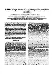
Figure 2: Constructing a DIMENSIONS Hierarchy: Temporal and Spatial Summarization
Figure 1: Feature Extraction in Sensor Networks Application
Sensors
Expected Rates
Seismic Monitoring [4]
Accelerometer
Micro-climate ing
Temperature, Light, Precipitation, Pressure, Humidity Acoustic, Video
Monitor-
Habitat Monitoring
Data
Data Requirements/Year
Expected Lifetime using Centralized Storage (approx)
30minutes seismic events per day per sensor 1 sample/minute/sensor
8Gb/year
Motea few weeks
MK-2[13]b few months
Expected Time to Storage Limit if all Raw data were stored (approx) Mote MK-2 few days 1 year
40Mb/year
few months
1 year
1 months
25 years
10 minutes of audio and 5 mins of video per day
1 Gb/year
few weeks
few months
few days
8 years
Table 1: Data Requirement estimates for Scientific Applications a Mote: b MK2:
Peak Current-25mA, Radio Baud Rate - 10Kbps effective, 4Mb storage, 2 AA batteries Peak Current-50mA, Radio Baud Rate - 10Kbps effective, 1Gb storage, 8 AA batteries
querying was proposed. Summaries are generated in a multi-resolution manner, corresponding to different spatial and temporal scales. Queries on such data are posed in a drill-down manner, i.e., they are first processed on coarse, highly compressed summaries corresponding to larger spatio-temporal volumes, and the approximate result obtained is used to focus on regions in the network are most likely to contain result set data. Wavelet-based summarization can potentially benefit query processing in three ways: (a) it produces a compact representation of data that highlights interesting features such as long-term trends, edges and significant anomalies and is, therefore, useful for general purpose query processing; (b) once generated, many spatiotemporal queries can be satisfied with negligible communication overhead by drill-down querying; and (c) aging (discarding) summaries selectively gracefully degrades query performance over time in storage-constrained networks. In this paper, we address the performance issues of this scheme. Specifically, given that storage is constrained, and communication is expensive, can we intelligently store and lookup summaries so as to maximize query accuracy? Our contribution in this paper is twofold: • We show that wavelet-based hierarchical summarization provides accurate responses to a broad spectrum of spatiotemporal queries with low communication overhead. Although a preliminary description of multi-resolution summarization was presented in ([11]), in this paper, we present comprehensive query surveys on an iPAQ-based implementation. • Second, we show that in a storage-constrained environment, graceful query degradation over time is achieved by networked aging of summaries, such that more useful summaries are retained longer. To our knowledge, no one has examined data aging in the context of highly distributed sensor systems. We present the design and implementation of DIMENSIONS on a linux platform. To evaluate the performance of our system, we consider queries posed on a geo-spatial dataset ([12]), which provides precipitation data from a medium-scale sparse sensor network.
2
2
DIMENSIONS Architectural Overview
We describe the architecture of our system in three parts: (a) the hierarchical wavelet processing that constructs lossy multiresolution summaries, (b) the typical usage of these summaries through drill-down queries, and (c) the data aging scheme that determines how summaries should be discarded, given their incremental benefit to drill-down queries and their storage requirements. Summarization and data aging are periodic processes, that repeat every epoch. The choice of an epoch is applicationspecific, for instance, if users of a micro-climate monitoring network ([1]) would like to query data at the end of every month, then a reasonable epoch would be a month. In practice, an epoch should at least be long enough to provide enough time for local raw data to accumulate for efficient summarization.
2.1
Multi-Resolution Summarization
We assume that our system will be used for a wide range of queries that search for patterns in data. Therefore, we use a summarization technique that is generally applicable, rather than optimizing for a specific query. Wavelets have well-understood properties for data compression and feature extraction and offer good data reduction while preserving dominant features in data for typical spatio-temporal datasets ([14, 15]). As sensor networks mature and their applications become better defined, more specialized summaries can be added to the family of multi-resolution summaries maintained in such a framework. Hierarchical processing using wavelets involves two phases. The first phase, temporal summarization, is cheap since it involves only computation at a single sensor, and incurs no communication overhead. This step consists of each node reducing the time-series data as much as possible by exploiting temporal redundancy in the signal. The spatial summarization phase constructs a hierarchical grid-based overlay, and uses spatio-temporal wavelet compression to re-summarize data at each level. Figure 2 illustrates its construction: at each higher level of the hierarchy, summaries encompass larger spatial scales, but are compressed more, and are therefore more lossy. At the highest level, one or a few nodes have a very lossy summary for all data in the network.
2.2
Drill-Down Querying
Drill-down queries on distributed wavelet summaries can dramatically reduce the cost of search. The term is borrowed from the data mining literature, where they are used extensively to process massive amounts of data. These queries operate by using a coarse summary as a hint to decide which finer summaries to process further. By restricting search to a small portion of a large data store, such queries can reduce processing overhead significantly. Our use of drill-downs is in a distributed context. Queries are injected into the network at the highest level of the hierarchy, and processed on a coarse highly compressed summary corresponding to a large spatio-temporal volume. The result of this processing is an approximate result that indicates which regions in the network are most likely to provide a more accurate response to the query. The query is forwarded to nodes that store summaries for these regions of the network, and processed on more detailed views of these sub-regions. This procedure continues until the query is routed to a few nodes at the lowest level of the hierarchy or until an accurate enough result is found at some interior node. Such query processing offers multiple benefits. When the target query result is sparsely distributed in a large network, query results can be obtained in a few steps(O(log4 n), where n is the number of nodes in the network), and with significantly less overhead than flooding a query to the entire network. Also, since the data is processed and stored once, the up front cost of storage can be amortized over multiple queries.
2.3
Networked Data Management
Providing a long-term query processing capability requires being able to store summaries for long deployment periods. In storage-constrained networks (Table 1), however, resources have to be allocated for storing new summaries by discarding older ones. While such constraints render it impossible to provide very high query accuracy for long durations, can we provide the user with gracefully degrading quality over time, such that better accuracy is obtained for queries about recent sensor data, and lower quality for older data? The goal of networked data management in our system is to age or discard summaries to effectively use network storage resources in a manner that gracefully degrades quality over time. Each summary represents a view of a spatial area for an epoch, and their aging renders such a view unavailable for query processing. For instance, storing only the highest level (level 3) summary in Figure 2, provides a condensed data representation of the entire network and consequently low storage overhead, but may not offer sufficiently accurate query responses. Storing a finer summary (level 2) in addition to the coarser one, enables an additional level of drill-down, and offers better accuracy, but incurs more storage overhead. A resource allocation scheme for such a system, thus, has to consider three factors: (a) the distributed storage resources in the network, (b) the compactness of a summary, measured in bytes per spatio-temporal volume and (c) the incremental query benefit obtained by having the summary.
3
We propose a progressive data aging strategy that uses an offline algorithm to determine system parameters for on-line operation. The offline storage allocation scheme determines how each node should apportion its local storage resources to different summaries. In this paper, we discuss several such allocation schemes that can be used depending on the availability of prior datasets. The output of this algorithm is a storage partitioning for each node that allocates its limited storage resources to summaries of various levels. Storage parameters determined from such an allocation scheme can be used to determine the ratios of storage requirements of summaries of various levels to one another. For example, in a three level hierarchy, a ratio of 1:1:1 means that one third of the total network storage is occupied by coarse, medium, and fine resolution summaries respectively. The DIMENSIONS search tree organizes summaries from coarsest at the root to finest at the leaves. In this tree, each parent can form a coarser spatio-temporal summary of a particular epoch from its four children’s’ finer summaries of that epoch. Considering only one epoch, the ratio, therefore, of coarsest to finest summaries in an n-level hierarchy is 1 : 4n . If we consider summarization over multiple epochs, and would like, for example, to store exactly as many coarsest summaries as finest summaries, then we would be able to maintain 4n times longer a history in coarse form than in fine form. Regardless of the ratio of allocation, to share the storage burden uniformly across all nodes in the network, we periodically reassign network nodes to logical search tree nodes.
2.4
Discussion
Our architectural description currently assumes that nodes in the network are arranged in a grid, or otherwise uniformly deployed. Sensor networks may not be carefully deployed, and more irregular topologies might be commonly seen. We are exploring techniques to relax this assumption. Random deployments can be approximated by grids by coarsening the grid sizes and interpolating for missing points. Work in wavelet lifting in irregular sampled datasets ( [16]) can be used to deal with this problem. While we choose to focus on storage issues in this paper, working with irregular topologies will be considered in future work. Our work assumes that there is a globally synchronized timebase that is available to relate data from different nodes. Unless this is available, data from different areas in the network cannot be processed using our techniques. A number of solutions exist to this problem, such as [17]. Periodic synchronization is necessary for any kind of useful sensing and monitoring task in the network and to relate events at different locations, so we assume that such a scheme will be in place. We impose two restrictions on the creation and storage of summaries in our current work that might change in future versions. First, we assume that all summaries at the same level are of equal size. While this constraint has the advantage of making communication balanced between different parts of the network, this may not be ideal for query accuracy, since it ignores the actual variations in the data in different regions of the network. In future work, we will consider error-based configurations, that look at correlation statistics to determine the amount of data to be transmitted at each level. Second, we assume that summaries are not progressively degraded by nodes that store them. This restriction can be relaxed, and can result in more graceful quality degradation by degrading in smaller steps. Such a mechanism can be introduced quite easily into the aging strategies that we discuss in this paper. We do not discuss how to determine the ideal hierarchy depth for a particular application. A hierarchy with a large number of levels might not be useful since the high-level summaries might be too coarse for useful query processing. For medium scale networks, such as the one that we consider, the number of levels (log4 N ) is presumably low (less than 5). For a much larger network, this question would need to be addressed.
3
System Implementation
In this section, we describe the implementation of DIMENSIONS on a linux-based network emulation platform ([18]). There are three major components to our system (shown in Figure 3): the wavelet transform coding used to construct the summaries, the local storage implementation that allocates storage to summaries from different levels, and the distributed quad-tree, which provides a system abstraction to support hierarchical storage and drill-down search.
3.1
Wavelet Codec
The wavelet codec software is based on a high-performance transform-based image codec for gray-scale images (freeware written by Geoff Davis ([19]). We extended this coder to perform 3D wavelet decomposition to suit our application. For our experiments, we use a 9/7 wavelet filter, uniform quantizer, arithmetic coder and near-optimal bit allocator. The 9/7 filter is one of the best known for wavelet compression, and especially for images. While the suitability of different filters to sensor data requires further study, this gives us a reliable initial choice of wavelet filter.
4
Sensor Data
1D
Increasing Query Accuracy
Wavelet Codec
Local
Distributed Quad Tree
3D
Local Storage Circular Buffer Per Level level N
level N−1
...
User−defined expected quality Graceful Quality Degradation Summaries Aged Simultaneously Only Coarsest Summary Stored
Increasing Time
Figure 3: Implementation Block Diagram
3.2
Figure 4: Providing graceful quality degradation by aging summaries
Local Storage
Local storage is implemented as circular buffers over berkeleydb (standard in glibc). Each summary is indexed by the level, quadrant, and epoch to which it corresponds. Every query on a summary involves first decompressing the summary, and then processing the query on the summary. The parameters of the local storage are determined using an aging strategy, that partitions the local storage between different summaries.
Choosing an Aging Strategy Depending on the aging strategy, the performance can be expected to vary considerably. Figure 4 shows two extreme aging strategies. At one extreme, only coarsest summaries are stored in the network, which, being compact, can be retained for long durations. However, query quality is low, irrespective of whether queries look at recent data or older data. At the other extreme, all summaries can be aged simultaneously, i.e., the coarsest summary is stored for the same amount of time as the finest summary. In this case, query quality is high, but all summaries can only be stored for a very short duration. A preferred aging strategy is a gracefully degrading strategy, where high query quality can be obtained for recent data, and low quality for older data. We assume in long-lived sensor networks that users are more likely to require fine-grained information about recent data than about older data. The parameters of the step function in Figure 4 depend on the desired query quality of the user. Such a function can be expected to be provided by a domain expert who has an idea of the usage patterns of the sensor network deployment. We define the notion of a user-specified aging function to describe how much error a user is willing to accept as data ages in the network (shown in Figure 4). Our goal is to approximate the user-specified aging function using a step function, that represents query degradations due to summaries being aged. How does one design an aging strategy? Different options might be possible depending on whether prior datasets are available for the application. In some scientific applications, a data gathering phase might precede full-fledged deployment (e.g.: James Reserve [1]), potentially providing such datasets. In other cases, there might be available data from previous wired deployments (e.g.: Seismic Monitoring [4]). These datasets can be used to train sensor calibration, signal processing and in our case, aging, parameters prior to deployment. The usefulness of a training procedure depends greatly on how well the training set represents the raw data for the algorithm being evaluated. For instance, if the environment at deployment has deviated considerably from its state during the training period, these parameters will not be effective. Ultimately, a training procedure should be on-line to continuously adapt to operating conditions. Systems, sometimes have to be deployed without training data. For instance, [20] describes sensor network deployments in remote locations, such as forests, and [7] discusses how motes may be deployed from an airplane for military applications. In the absence of training datasets, we will have to design data-independent heuristics to age summaries for long-term deployment. The intent of this study is to see how to design algorithms for aging in two cases: with training and without training. For the case when prior datasets are available, we formulate an optimization problem that can be used to compute aging parameters, both for a baseline, omniscient scheme that uses full information, and for a training-based scheme that operates on a training set. For deployments where no prior data is available, we describe a greedy aging strategy.
Formulating the Aging Optimization Problem In this section, we present an informal description of the optimization problem, objective function, and constraints. A more detailed treatment can be obtained from Appendix A.
5
Symbol S f (t) Q(t) Sumi
xi Agei
N rb
Parameter Local storage constraint The (user-specified) desired aging function Resulting step function Size of each summary for level i. Sum0 is the raw data at a node, for all other levels, Sumi is the size of a quadrant worth of data Number of summaries of level i stored at each node Aging Parameter for level i, i.e., duration in the past for which a level i summary is available Number of nodes in the network Resolution bias of the greedy algorithm
Level
Number of Clusterheads
Size of Summaries
0 (finest) 1 (finer) 2 (coarsest)
16 4 1
1 2 4
Rate of Generation (number of summaries per epoch) 16 4 1
Storage allocated per node (epochs)
Age (epochs)
2 2 3
2 8 48
Table 3: Example of a greedy algorithm for a 16 node network
Table 2: Parameters for the Aging Problem Consider the aging problem in a n-level DIMENSIONS hierarchy, where the lowest level (0) corresponds to lossless raw data and the highest level (n − 1) corresponds to the lossiest compressed summary for the entire network. The user provides a monotonically decreasing user-defined aging function, such as the one shown in Figure 4. The objective of the optimization is to evaluate how each node allocates its local storage to summaries for different levels. This can be used to calculate the age of summaries at each level, defined at a particular instant as how far into the past summaries can be expected to be available on-line for that level. Objective Function: We would like to minimize the worst-case performance, given a particular aging strategy. The performance metric that we choose is the instantaneous quality difference (qdiff), defined as the difference between the user-specified aging function and the achieved query accuracy at any instant in time (shown in Figure 10). The objective function, thus, seeks to minimize the maximum instantaneous quality difference over all time. M in0≤t≤T (M ax (qdiff(t)))
(1)
Drill-Down Constraint: Queries are spatio-temporal and strictly drill-down, i.e., they terminate at a level where no summary is available for the requested temporal duration of the query. In other words, it is not useful to retain a summary at a lower level in the hierarchy if a higher level summary is not present, since these cannot be used by drill-down queries. Storage Constraint: Each node has a finite amount of storage, which limits the number of summaries of each level that it can store. The number of summaries of each level maintained at a node is an integer variable, since a node cannot maintain a fractional number of summaries. The age of summaries at a level can be computed from this by considering the total number of nodes in the network and the rate at which summaries at the level are generated. Additional Constraints: In formulating the above problem, we consider only drill-down queries and a network of homogeneous devices with identical storage limitations. These constraints might not always be true. For instance, queries may look at intermediate summaries directly, without drilling down. Previous research has proposed a tiered model for sensor deployments ([21]), where nodes at higher tiers have more storage and energy resources than nodes at lower tiers. While we do not consider such constraints in this work, our model can be easily extended to incorporate them. The optimization problem is linear when a user-specified linear aging function is chosen, and non-linear otherwise. While many instances of non-linear optimizations can be solved using state of the art solvers, we will consider only the linear case in this study. We next describe three algorithms for aging, the first is a baseline optimal scheme that operates on the entire dataset; the second operates on a training set, and the third is data-independent.
Aging Algorithms Omniscient Algorithm: An omniscient scheme choses the best possible aging parameters for each query. To compute the performance of such a scheme, we use the query quality from offline processing of the entire dataset, and evaluate the optimization function on these results. Omniscience comes at a cost that makes it impractical for deployment. It is provided as a baseline strategy for comparative purposes. Training-based Algorithm: This algorithm uses a similar approach, but operates only on a short training dataset. This dataset is used to model query accuracy during deployment. The optimization procedure is performed on this predicted model to determine an aging strategy. Greedy Algorithm: Algorithm 1 describes a greedy procedure that can be used in the absence of prior datasets. When available storage is larger than the size of the smallest summary, the scheme tries to allocate summaries starting with the coarsest one. We use a parameter, resolution bias (rb), to prioritize the allocation of storage to various resolution summaries. The ratio of the coarsest summaries to summaries that are i levels finer are rbi . For instance, in a three-level hierarchy (Table 3), a resolution bias of two means that for every coarse summary that is stored, two of finer, and four of the finest summaries are attempted to be allocated. This parameter is used to control how gradually we would like the step function (in Figure 4) to decay.
6
: S: local storage capacity; N : number of nodes in the network, therefore, log4 N levels; Sumi : the size of a summary at level i Result : Assignment of number of summaries of each level to store locally while at least the smallest summary can fit into the remaining storage space do Assign Summaries starting from the coarsest; for level i = log4 N down to 1 do if storage is available then allocate rblog4 N −i summaries of level i; Data
Algorithm 1: Greedy Algorithm Pseudocode Time
present
past
2 epochs
0
0
fine
...
1
1
Resolution level 12 epochs 1
2
2
2
coarse 32
8 epochs 1 Second Pass
First Pass
2
1
0
2
1
0
Third Pass
48 epochs 2
2
...
Time
past
2
4 epochs 0
epochs 2
... ...
present
0
0
0
fine
1
1
1
Resolution level
2
2
2
Time
past
coarse
present
...
0
0
16 epochs 1
...
0 1
1
1
Resolution level
16 epochs 2
...
2
2
2
coarse
6 epochs
fine
2
Local Storage Capacity = 18 units
Figure 5: Local Re(c) Short Duration, High Ac(b) Medium Duration, source Allocation using (a) Long Duration, Low Accucuracy Medium Accuracy the Greedy Algorithm racy (rb=1). 3 coarsest, 2 finer, and 2 finest sum- Figure 6: Different global resource allocations that can result from a local allocation promaries are allocated cedure. For instance Figure 6(a) corresponds to the local allocation in Figure 3.2. A single coarse summary is generated every epoch. In a network of 16 nodes, each of which allocates, say, 3 storage slots to coarse summaries, a total of 48 storage slots are available. Thus, the age of a coarse summary is 48 epochs. Similar calculations can be done for other summaries The procedure results in progressive aging of summaries in the network. Since coarse summaries are generated less frequently than fine summaries, if, as seen in Section 2.3, we would like to store as many coarse summaries as fine summaries, the coarser summary will have a greater aging period than finer ones. For instance, consider a greedy allocation with resolution bias of 1 in a 16-node network (such as Figure 2) with parameters provided in Table 3. There are three levels in such a hierarchy, with 16 clusterheads at level 0 (every node), 4 at level 1, and 1 at level 2. Consider an instance where the local storage capacity is 18 units and the sizes of each summary are as shown in Table 3. The greedy allocation scheme allocates summaries starting with the coarsest level as shown in Figure 3.2. In the first and second passes, one of each summary is allocated, and in the third, one coarsest summary is allocated. Thus, a total of 3 coarsest, 2 finer, and 2 finest summary are allocated to each node. To calculate the age of summaries at each level, we use the fact that the network has 16 nodes, thus, a total of 16 ∗ 3 = 48 storage slots are allocated to level 2, 32 slots to level 1, and 32 slots to level 0. Since 1 coarsest (level 2) summary is generated per-epoch, the age of a level 2 summary is 48 epochs. Similarly, the ages of level 1 and level 0 are 8 and 2 epochs respectively (Table 3). This aging sequence is shown in Figure 6(a). Such an allocation favors the coarsest summary much more than the finer ones. Thus, the network supports very long-term querying (48 epochs), but with high error for queries that delve into older data. Other allocations can be considered under the same resource limitations. Figure 6(b) shows an allocation that balances detail and duration, whereas the allocation in Figure 6(c) favors detail over duration.
3.3
Distributed Quad Tree
The local storage partitioning discussed in the previous section allocates some portion of the storage at each node to summaries for each level. The Distributed Quad Tree (DQT) describes the routing and cluster-head selection scheme that assigns summaries to each node in the network such that the allocated networked storage is appropriately utilized. The DQT is a routing overlay that decomposes the network space hierarchically into quadrants, and assigns a rendezvous node to each quadrant in the manner suggested by GHT’s structured replication ([22]). By using a geographical hash function, a globally shared convention for selecting nodes, the construction of the tree overlay requires no setup communication, eliminating the overhead of clusterhead election and global consensus. In this sense, it is a good choice for energy constrained sensor networks.
7
The DQT is a rooted spatially distributed search tree and is defined recursively as follows: • Given a bounding rectangle R and a globally known constant c, the geographic hash function h(R, c) → (x, y) hashes c to a location in R. The node physically closest to (x, y) is selected as the storage rendezvous for R. • The root node of the DQT overlay is the rendezvous node selected when the minimum enclosing rectangle of the network, Rb , is used as input to h. • Every interior node in the overlay (including the root) has exactly four children, each covering separate equally-sized quadrants of its parent’s bounding rectangle. The bounding rectangles of these quadrants are used as input to h to determine the locations of these children in the same manner in which the root node was chosen. This recursion terminates at a globally-known pre-specified depth. The DQT implementation provides four services to applications using it: Abstraction. The client interface allows communication to be specified in terms of tree options such as ascend to parent or descend to a particular child instead of in terms of nodes in the network. The DQT supports the following operations: route up, route down, and to location. The operation to location provides applications with a means to bypass the quad tree overlay and geographically route directly to named locations. These operations can be used both to construct and distribute wavelet summaries in the network, and to route drill-down queries to specified destinations. route up is used in the storage process; route down is used by queries as they descend the tree in search of results; and to location returns data directly from the nodes storing parts of the result set to the query sink. Rendezvous Selection. DQT provides a geographic hashing scheme that translates a globally known constant and a bounding rectangle into geographic coordinates. It relies on an underlying geographically informed routing protocol that understands the semantics “route to the node that is geographically closest to location (x,y)” to select and deliver messages to rendezvous nodes. The extension of GPSR that is presented in [22] is such a protocol. In our implementation, however, we used a link-state geographic routing protocol enhanced to support these semantics. Since the population of link-state routing tables require the dissemination of each node’s link state to every other, it may provide adequate routing for relatively small networks, but it is not a scalable solution for the long run. We therefore plan to port the GPSR and its GHT enhancement to our architecture. Rendezvous Rotation for Load Sharing. DQT supports a time varying version of the geographic hash so that the particular nodes chosen for rendezvous in the DQT overlay change at a specified frequency. This is implemented by adding a counter to the input of the hash that increments at the rotation frequency. This serves two purposes: communication balancing and storage balancing. Communication balancing avoids the loss of sensing coverage, and storage balancing allows us to store summaries longer, therefore providing better performance for query processing in storage-limited networks. Reliability. DQT has an ack/retransmit timeout mechanism to provide reliable communication in the tree overlay.
4
Experimental Evaluation
Since dense wireless sensor network datasets that are available lack sufficient temporal and spatial richness , we use a geospatial precipitation dataset [12] for our current performance studies. This dataset provides a 15 x 12 grid of daily precipitation data for forty five years, where adjacent grid points are 50 kilometers apart. Both the spatial and temporal sampling are much lower than what we would expect in a typical sensor network deployment (Table 1). While the data sizes and scale would be expected to be larger in practice, this dataset has edges and exhibits spatio-temporal correlations, both of which are useful to understand and evaluate our algorithms. Since the spatial scale of the dataset is low, the primary form of processing along the hierarchy was repeated temporal processing.
4.1
Communication Overhead
Our objective is to evaluate whether the system can process and organize summaries in a DIMENSIONS hierarchy with low communication overhead. To construct summaries, we used an epoch of three years i.e., the summary construction process repeats every three years. The choice of a large time-period was due to the temporal infrequency of samples. Each node in the network would have 1095 samples to process every three years, enough to offer reasonable temporal compression benefit. In a typical deployment (Table 1), where nodes generate more data, the epoch would be much shorter. The total communication overhead for summaries at each level is shown in Table 4. We used compression ratios 1:6:12:24:48 for successive levels of the hierarchy, in terms of the raw data size, and the results from the codec were within 4% the input compression parameters. The standard deviation results from the fact that the dimensions of the grid are not perfectly dyadic (power of two) and therefore, some clusterheads aggregate more data than others.
4.2
Query Performance
Can good query accuracy be obtained by processing summaries constructed with low communication overhead? We address this question by evaluating the performance of drill-down processing on a broad set of queries as shown in Table 5. Each of
8
Hierarchy Level
Raw 0 1 2 3
Data
Size (bytes) 2190 367.1 689.1 1400.1 1933.5
Type GlobalDailyMax
Compression Ratio (Compressed Data Size/Raw Data)
Conf Int 0 0.11577 17.661 24.417 174.2
GlobalYearlyMax 1 5.97 11.91 23.46 50.9
Table 4: Communication Overhead per Level
LocalYearlyMean GlobalYearlyEdge
Query What is the maximum daily precipitation for year X? What is the maximum annual precipitation for year X? What is the mean annual precipitation for year X at location Y? Find nodes along the boundary between low and high precipitation areas for year X
Table 5: Spatio-temporal queries posed on Precipitation Dataset
these queries, GlobalDailyMax, GlobalYearlyMax, LocalYearlyMean, and GlobalYearlyEdge is named after the spatial and temporal scale, and the feature that they process. We pose three kinds of queries that involve different extents of spatio-temporal processing that evaluate both advantages and limitations of wavelet compression. The GlobalYearlyEdge and LocalYearlyMean queries explore features for which wavelet processing is typically well suited. The Max queries (GlobalDailyMax, GlobalYearlyMax) looks at the Max values at different temporal scales. The GlobalYearlyMax query looks at the maximum yearly precipitation in the entire network, while the GlobalDailyMax queries for the daily global maximum. Wavelet processing does not preserve maxima very well in practice. To evaluate performance, each of these queries was posed for every year of data. Thus, there were forty five queries of each type that were processed, and the following results are averaged over these query results. The query accuracy for a drill-down query that terminates at level i is defined as the fraction error i.e., the difference of the measured drill-down result and the real result over raw data over the real result (measured - real/real). Figure 4.2 shows the variation of query quality for queries defined in Table 5 for different levels of drill-down. Both the LocalYearlyMean query and the two Max queries are processed as regular drill-down queries. The query is processed on the coarsest summary to compute the quadrant to drill-down, and is forwarded to the clusterhead for the quadrant. The GlobalYearlyEdge query tries to find nodes in the network through which an edge passes, and involves a more complex drill-down sequence. This query is first processed by the highest-level cluster-head, which has a summary covering the spatial extent of the entire network. The cluster-head uses a standard canny edge detector to determine the edge in its stored summary, and fills a bitmap with the edge map. The query and the edge bitmap are then forwarded to all quadrants that the edge passes through. The cluster-heads for these quadrants run a canny detector on their data, and update the edge bitmap with a more exact version of the edge. The drill-down stops when no edge is visible, and the edge bitmap is passed back up, and combined to obtain the answer to the query. As expected, the GlobalYearlyEdge and LocalYearlyMean Queries perform very well on the compressed data. For the GlobalYearlyEdge query, we measure error as the fraction of nodes missed from the real edge. The error is within 5%, even when the query terminates at the highest level summary, and does not improve as a result of further drill-down. This result is consistent with what one would expect for edge detection, the edge is more visible in a lower resolution (and consequently, higher level) view, and becomes more difficult to observe at lower levels of the hierarchy. In a larger network, with more levels, improvement might be observed using drill-down. Relative error for the LocalYearlyMean query reduces sharply from around 50% for the level 4 summary to almost 0% for the level 1 summary. The error for Max queries shows similar behavior as well, although it improves less with increasing drill-down levels. The error for GlobalDailyMax query reduces from 50% to 12% as the query drills down from the level 4 to the level 1 summary. GlobalYearlyMax queries follow a similar trend, the level 4 summary has error 30%, whereas drilling down to the level 1 reduces error to 8%. The communication overhead of posing these queries is extremely low. All the queries that we look at drill-down into very few branch (usually one) at each level of the hierarchy, bounding the maximum number of nodes queried by O(log4 N ) i.e., only around 5% of the network is queried for the result.
4.3
Performance of Aging Strategies
As shown in the previous section, different summaries contribute differently to the overall query quality, with the top-level summary contributing maximum. For instance, in the case of the GlobalDailyMax query, query error reduces by 50% by storing only the level 4 summary. Adding an additional level of summaries decreases error by 15%, and so on till storing raw data results in 0% error. This trend motivates the aging problem, which allocates storage to different summaries based on their marginal benefit to query processing, and their storage utilization. In this section, we consider three of the queries from Section 4.2, omitting the GlobalYearlyEdge query, since it is not impacted by having any more than the coarsest summary. We consider linear aging functions of the form QueryAccuracy = 1 − time/DecayRate. The DecayRate is varied between 100 and 200, and determines whether the user would like a fast decay of query accuracy over time, or a slower decay.
9
Error vs Level GlobalDailyMax Query GlobalYearlyMax Query LocalYearlyMean Query
0.6
Storage CDF 0.14
Communications CDF 0.06
Rotating Hash Fixed at Centers
0.5 0.4 0.3 0.2
0.1
0.08
0.06
0.04
0.1
0.02
0
0
0
1
2 3 Level in hierarchy where query terminates
4
5
Figure 7: Query error decreases as they drill-down to lower levels of hierarchy. Summaries at lower levels typically contribute less to reducing query error than higher level summaries.
Fraction of Total Bytes Sent and Received
0.12 Fraction of Total Bytes in Storage
Fraction Error (Measured - Real/Real)
0.7
0
0.2
0.4 0.6 Fraction of Nodes
(a) Storage Overhead
0.8
1
Rotating Hash Fixed at Centers
0.05
0.04
0.03
0.02
0.01
0
0
0.2
0.4 0.6 Fraction of Nodes
0.8
1
(b) Communication Overhead
Figure 8: Distributed Quad Tree Performance on a 64-node network: Storage and Communication is balanced better than a strict hierarchical approach.
The performance metric that we will use for our evaluation is max(qdiff), which represents the maximum difference between user-specified query quality and the achieved query quality. We address two questions in this evaluation. First, given a storage constrained network, what is the lower bound on max(qdiff)? We evaluate this by looking at the performance of the omniscient scheme that operates with full knowledge of dataset and queries. Second, we evaluate two practical schemes, training-based and greedy, to determine which scheme performs better, and how far from optimal they perform.
Establishing a Lower Bound for Query Error An omniscient scheme operates on the entire dataset, and thus, has full knowledge of the query error obtained by drilling down to different levels of the hierarchy (Figure 4.2). The optimal aging strategy may then be computed by feeding appropriate parameters to the optimization routine discussed in Section 3.2. Figure 9 shows the performance of this scheme for one instance of a user-specified linear aging function (DecayRate = 100). In networks composed of nodes with low local storage capacities, the error is high since only the coarsest summaries can be stored in the network. As shown in Table 6, the error from the coarsest summaries ranges from 30% to 50% for different queries. As the local storage capacity increases, however, the optimal algorithm performs dramatically better, until 0% error is achieved with approximately 16KB to 20KB of storage. Full knowledge is impossible in practice and we use the omniscient scheme as a basis for comparing how practical schemes such as training and greedy schemes perform.
Evaluating Training using Limited Information In our evaluation of the training-based scheme, two epochs of data available prior to system deployment, are used to predict the query accuracy for the entire dataset. Such data might be expected to be available if a data gathering phase preceded actual deployment. Summaries are constructed over the training set, and queries in Table 5 are posed over these summaries. Ideally, the error obtained from the training set would mirror error seen by the omniscient scheme. Table 6 shows that the predicted error from the training set is typically within 2%-3% of the query quality seen by the omniscient scheme, but is almost 10% off in the worst case (Max queries over finer summaries). Thus, the training set is only moderately representative of the entire dataset. Unlike the omniscient idealized algorithm, the training scheme cannot choose a resource allocation per-query. In a practical deployment, a single allocation scheme would be required to perform well for a variety of queries. Therefore, the training scheme uses the predicted error for different queries to compute a cumulative error metric as shown in Equation 2. The cumulative error can be fed to the optimization function to evaluate aging parameters for different summaries. Σquery types Err2 epochs (level i) (2) N umber of query types Figure 9 shows the result of such a resource allocation scheme. The training curve follows the omniscient storage allocation curve for both the Max queries, but converges slower for the Mean query. Average error (Table 7) shows a similar trend for all choices of the DecayRate. While training performs within 0.2% of optimal for the GlobalDailyMax and GlobalYearlyMax queries, the error grows as large as 6% for the LocalYearlyMean query. The variability in performance for different queries can be explained by the fact that the cumulative error (Table 6) is more representative of the actual error for the Max queries than the Mean query. Errcumulative (level i) =
10
Level till which drilled down
GlobalYearlyMax Omniscient 9.1% 11.6% 18.1% 33.6%
1 2 3 4
GlobalDailyMax
Training 15.6% 17% 18.8% 30.9%
Omniscient 13.4% 16.9% 26.6% 48.7%
LocalYearlyMean
Training 22.3% 24.4% 28% 45.8%
Omniscient 0.1% 5.9% 20.9% 48.4%
Cumulative Training Error
Training 1.1% 6.8% 24.1% 56.7%
13% 16.1% 23.6% 44.5%
Table 6: Comparing the error in Omniscient (entire) Dataset vs Training (first 6 years) Dataset GlobalDailyMax Aging Parameters
0.4 0.35 0.3 0.25 0.2 0.15 0.1
0.25 0.2 0.15 0.1
Omniscient Training Greedy: duration Greedy: balanced Greedy: detail
0.8
0.6
0.4
0.2
0.05
0.05 0
LocalYearlyMean Aging Parameters 1
Omniscient Training Greedy: duration Greedy: balanced Greedy: detail
0.3 Fraction Error (measured-real/real)
Fraction Error (measured-real/real)
GlobalYearlyMax Aging Parameters 0.35
Omniscient Training Greedy: duration Greedy: balanced Greedy: detail
Fraction Error (measured-real/real)
0.5 0.45
0
10
20
30
40 50 60 Local Storage Size (KB)
70
80
(a) GlobalDailyMax
90
100
0
0
10
20
30
40 50 60 Local Storage Size (KB)
70
80
(b) GlobalYearlyMax
90
100
0
0
10
20
30
40 50 60 Local Storage Size (KB)
70
80
90
100
(c) LocalYearlyMean
Figure 9: Comparison of Omniscient, Training and Greedy strategies for Max and Mean queries (DecayRate=100) Greedy Algorithm The greedy scheme (Algorithm 1) does not assume the availability of training datasets but instead uses a resolution bias parameter to decide how to allocate storage between different summaries. We use three settings for this parameter, a low resolution bias (one), that favors duration over detail, a medium bias (two), that balances both duration and detail, and a high bias (four), that favors detail over duration. Table 7 shows that the choice of resolution bias significantly affects error for the greedy algorithm. In all cases, a medium choice of bias (balanced) is significantly better than both a low (duration) and high (detail) bias. For instance, in the case of the GlobalDailyMax query, while the greedy algorithm with bias of either duration or detail performs about 10% worse than training and omniscient schemes, a balanced bias performs only about 1% worse. Figure 9 shows that the qdifffor duration and detail bias converges to 0% very slowly as well. This result can be understood by looking at the relationship between resolution bias, and the aging parameters for different summaries (Figure 3.2). A low value of resolution bias (duration) results in more storage being approtioned to coarser summaries, thus biasing towards very long duration, but low accuracy (Figure 6(a)). The maximum user error (max(qdiff))is observed for queries that look at recent data, where the user expects high accuracy, but the system can only provide coarse summaries. In contrast, a higher value for resolution bias (detail) allocates storage such that all summaries live for approximately equal periods of time in the network. The error is low, but so is the age of all summaries (Figure 6(c)). Queries on old data will result in a large max(qdiff) because summaries will be unavailable in the network for old data. Thus, as we vary the resolution bias between these extremes (0 to 4), we get different results from the greedy algorithm. An ideal choice of this parameter, such as rb = 2 (balanced), would lie between these extremes, and results in more gradual aging of summaries (Figure 6(b)).
Discussion We evaluate the sensitivity of our study to other system parameters, specifically, the choice of the user-defined aging function and the training period. How does the fact that a user wishes for a slower decay of query accuracy over time or a faster decay over time (Figure 4), affect the performance of the aging schemes? Table 7 shows that as the aging function goes from fast to slow, the error increases consistently for all schemes, since it is increasingly difficult to find a resource allocation that satisfies the user requirements. The relative performance of different schemes, however, remains unaffected by this parameter. Changing the training period to one epoch instead of two did not significantly change results either, and we do not present the results in this section. We see that for a suitable choice of parameters, both the training-based and the greedy scheme perform within 1% of optimal, and are suitable for most deployments. The training scheme outperforms the greedy scheme, but not significantly when a medium (balanced) resolution bias is chosen for the latter.
11
User-defined aging function DecayRate
GlobalDailyMax
Omni 100 (Fast) 150 (Gradual) 200 (Slow)
1.7% 2.3% 3.1%
Train 1.72% 2.4% 3.3%
Greedy (rb) duration balanced 6.0% 2.7% 8.6% 3.2% 10.3% 3.9%
GlobalYearlyMax
Omni detail 8.3% 8.5% 13.2%
1% 1.2% 1.8%
Train 1% 1.3% 2%
Greedy (rb) duration balanced 2.8% 1.8% 4.1% 1.9% 5.3% 2.7%
LocalYearlyMean
detail 5.5% 5.6% 10.8%
Omni
Train
1.3% 2.3% 3.5%
3.6% 6.4% 9%
Greedy (rb) duration balanced 6.4% 4.6% 9.9% 8.7% 13.6% 13.1%
detail 8% 8.5% 15.1%
Table 7: Sensitivity Analysis (AvgError = Average(0≤S≤100) QueryError(S) where S is local storage capacity in KB)
4.4
Performance of the Distributed Quad-Tree
To quantify the benefit provided by our load-balanced DQT implementation, we compare the communication and storage overhead of propagating data up the tree using rotating hash nodes against having nodes fixed at the centers of their covering rectangles. The study was done in the Emstar simulation framework ([18]), on a 8x8 grid topology, where each node has at most 8 neighbors. Each node generates the amount of data provided in Table 4, and picks a different hash location periodically as described in Section 3.3. Root nodes rotate at a rate of once every 10 epochs. A tree node i levels below the root rotates at a fewquency 2−i times that of the root. The cumulative distributions in Figures 8(b) and 8(a) show that rotating hash nodes incurs approximately the same total communication overhead as picking center nodes, but does a much better job of balancing both the communication and storage load. Communication load (Figure 8(b)) is not entirely balanced in this study because of limitations of a finite grid, and nodes in the middle of the grid (or at the center of any ad-hoc network), being subjected to more multihop communication overhead than other nodes. In an longer simulation on a larger scale network, we would expect the communication load to be more uniformly balanced in the network. While Figure 8(a) shows that storage balancing is close to uniformly balanced, it is clearly not the same at each node. This is to be expected since the hash function is probabilistic, and there is a finite probability of the same node being selected more (or less) than the expected number of times. In an irregular network, storage balancing would depend on the spatial density of node deployment as well. How does this impact aging parameters of the system? Consider an example where a node were to store summaries for a certain level for 8 epochs. If the frequency of rotating clusterheads were chosen to be once every 8 epochs, there is a finite probability that the same node is hashed to twice within the aging period, thus, resulting in the loss of summaries. Such a situation can be mitigated by choosing the rotation period to be faster than the number of summaries stored at each node. For instance, if the frequency of rotation is once every 2 epochs, then, better storage balancing can be achieved. In practice, since nodes will store many summaries, faster rotation will also balance communication load better.
5 Related Work We briefly describe the rationale behind our design choice to use wavelets, and proceed to describe a broad spectrum of related work. Survey of Data Compression and Representation Techniques. Techniques for data and signal compression abound. Typical lossless data compression techniques include huffman, arithmetic encodings, the Lempel-Ziv coder, etc. These techniques reduce data by a factor of two to ten in practice, and rarely provide the compression ratios of hundreds that we would like in our system. Lossy schemes, on the other hand, can be tuned to compress data to fit communication requirements in sensor networks. Wavelets decompose the data recursively into various time and frequency scales, and provides a good representation of both time and frequency content in a signal. This flexibility has been the primary reason behind the popularity of wavelets in signal and image compression, time-series data mining, and approximate querying [23, 24]. Wavelet compression tends to preserve interesting features such as edges and succinctly captures long-term behavior, and consequently provides a data representation ideal for spatio-temporal querying. Its benefit for edge and boundary detection stems from two properties: (a) subband coding preserves sharp changes at various scales, thus providing a good representation of edges and (b) multi-scale techniques are useful to detect edges that may be visible at different spatio-temporal scales. Distributed Data Storage. Distributed databases and data storage have been extensively studied in the context of the wide-area Internet. Aging of web-pages is particularly important for web-cache performance and has, therefore, been explored by researchers (eg: [25]). While similar in motivation, these systems differ from ours in many significant respects: (a) web pages are not known to exhibit spatial correlations, (b) they are designed for a much more resource-rich infrastructure, and (c) bandwidth, while limited, is a non-depletable resource unlike energy. Data Centric Storage (DCS [9]) is a system that extends primitives used in the peer-to-peer Content Addressable Networks system to provide a geographic hash table (GHT [22])-based high-level event storage in sensor networks. DCS assumes that an event description exists a priori, and therefore, event detections can computed in a distributed manner within the network.
12
The system is responsible for storing these detections (called observations) in a distributed framework for easy access. DIMENSIONS is designed for data mining, and does not assume a priori knowledge of event signatures. Thus, it involves mining massive spatio-temporal datasets, which is not the focus of DCS. The distributed storage aspects of our system have similarities to the techniques used in DCS, and we extend this scheme in our DQT implementation. Data Mining. Geographic Information Systems (GIS) deal with data that exhibits spatio-temporal correlations, but the processing is centralized, and algorithms are driven by the need to reduce search cost, typically by optimizing disk access latency. Some of these approaches ([23, 24, 26]) propose the construction of wavelet synopses, for fast processing of range-sum queries. Many of the techniques proposed for approximate querying and data mining have informed the coding techniques that we choose in our system. An interesting example of a distributed infrastructure for wide-area data mining of sensor data is Astrolabe [27], which proposes a hierarchical data mining approach that is similar in motivation and design to DIMENSIONS. Astrolabe hierarchically aggregates data, and uses a drill-down approach. There are three key differences between Astrolabe and our work: (a) Astrolabe is a generic platform, and does not specify an aggregation function to use, while our system is built upon being able to do multi-resolution wavelet processing in a distributed framework. (b) Astrolabe is designed for the wide-area Internet and therefore assumes less stringent bandwidth constraints. It uses bimodal multicast as the communication framework, which ensures very high reliability, but incurs high communication overhead. (c) The storage constraints are not as stringent in a wired network and are, therefore, not addressed. Sensor Network Databases. In recent years, many database mechanisms have been extended to sensor network data querying. Systems such as Diffusion [8], Cougar [28] and TinyDB [10] use in-network processing techniques. Diffusion provides a general framework for routing and in-network processing. It’s query mechanism is simply to flood an interest to all network nodes. Its efficiency comes in the way it is designed to process matching data in a hop-by-hop fashion on the return path, potentially reducing redundancy while transforming the data from raw time series information into a more compact and sematically richer representation. When multiple data sources respond to a query, Diffusion exploits the property that data generated from spatially proximal nodes is likely to be correlated. While Diffusion takes a dynamic approach to in-network processing, where data can be combined anywhere along the routing path, Cougar proposes a static model, where a centrally computed query plan decides where to place joins within the network. Finally, TinyDB provides a platform for resourceconstrained devices, and provides a programming interface to create new queries, and inject them into the network. The above approaches operate under the assumption that event description is known a priori, and that queries are explicitly defined for these event descriptions. Our system is designed to look for and find patterns in data.
6
Conclusion
Ideally, a search and storage system for sensor networks should have the following properties: (a) low communication overhead, (b) efficient search for a broad range of queries, and (c) long-term storage capability. In this paper, we present the design and evaluation of DIMENSIONS, a system that constructs multi-resolution summaries and progressively ages them to meet these goals. This system uses wavelet compression techniques to construct summaries at different spatial resolutions, that can be queried efficiently using drill-down techniques. We demonstrate the generality of our system by studying the query accuracy for a variety of queries on a wide-area precipitation sensor dataset. A significant contribution of this work is extending our system to storage-constrained large-scale sensor networks. We use a combination of progressive aging of summaries, and load-sharing by cluster-rotation to achieve long-term query processing under such constraints. Our proposal for progressive aging includes schemes that are applicable to a spectrum of application deployment conditions: a training algorithm where training sets can be obtained, and a greedy algorithm for others. A comparison shows that both the training and greedy scheme perform within 2% of an optimal scheme. While the training scheme performs better than the greedy scheme in practice, the latter performs within 1% of training for an appropriate choice of aging parameters. We demonstrate the load-sharing properties of our system in a sensor network emulator. In our future work, our primary focus will be deploying our system in a real sensor network deployment scenario.
A
Aging Optimization Problem Formulation
We’re given a user-defined aging function, f (t), which represents the query degradation that the user is willing to accept. Such functions will typically be expected to be monotonically decreasing (eg: Figure 4, i.e., expected query quality goes down as data is stored for a longer period of time. Table 2 describes the different parameters in our optimization problem.
Objective Function We wish to minimize qdiffover all time as described in Section 3.2 M in0≤t≤T {M ax qdiff(t)}
13
(3)
Points at which instantaneous quality difference is evaluated
~
H
~
2
~
2
2
H
Query Accuracy
G ~
2
~
2
A3
~
2
D3
G
S
G
H
D2
D1
Level 1
Level 2
( Finest Level )
Level 3 ( Coarsest Level )
S 3D dyadic subband decomposition
A3
D1
D2
Time
D3
C’
Figure 11: Dyadic Wavelet Analysis
Figure 10: Objective Function
For a monotonically decreasing user-specified aging function, qdiffneeds to be evaluated only at a few points (as shown in Figure 10). The points corresponds to the aging criteria for each of the summaries in the network. As can be seen, the value of qdiffat all other points is greater than or equal to the value at these points. M in0≤i≤n {M ax qdiff(Agei )}
(4)
can be linearized by introducing a new parameter γ M in0≤i≤n {γ}
(5)
qdiff(Agei ) ≤ γ ∀ i
(6)
Constraints • Drill-Down Constraint: Queries are spatio-temporal and strictly drill-down, i.e. they terminate at a level where no summary is available for the requested temporal duration of the query i.e., Agei+1 ≥ Agei ∀ i > 0 • Strorage Constraint: The sum of all summaries stored at each node is less than its total storage i.e., Σ0≤i≤n Sumi xi ≤ S • Aging Constraint: The age of summaries can be evaluated from the local allocations, xi , since we know the number of clusterheads at each level of the hierarchy. Since there are 4log4 N −i clusterheads at level i, Agei = xi 4i
B
Wavelet Subband Compression
In this appendix, we provide a brief, high-level overview of the steps involved in wavelet summarization. From a high level, there are two steps involved: Step 1: Decomposition The wavelet decomposition of a multi-dimensional signal array, S, involves obtaining a set of C 0 wavelet coefficients using a subband decomposition, as shown in Figure 11. The signal S is passed through a low-pass filter (H) and a high pass filter (G) recursively. After each decomposition, the low pass and high pass results are sub-sampled by 2 i.e., every second sample is dropped. The resulting decomposed signal, C 0 , is composed of the approximation coefficients (A) and the detail coefficients (D). This step is typically a lossless decomposition and the original signal array S can be perfectly reconstructed from C 0 coefficients. Step 2: Selecting Coefficients The array C 0 typically has a large number of small and insignificant coefficients, and can be made into a sparse array, C, by appropriate lossy coefficient selection. Many well-known techniques exist for coefficient selection. Typical wavelet compression mechanisms such as JPEG2000 image coding [29] process the data using a combination of thresholding, quantization and weighting subbands, thereby reducing the data into a sparse matrix. Lossless compression schemes such as Run-length Encoding (RLE) are then employed to exploit contiguous runs of numbers in the sparse matrix. Finally, a lossless entropy encoding step such as huffman encoding is applied to obtain the final compressed array. Compression parameters are typically chosen based on different cost metrics, including communication overhead, query performance, and mean square signal error.
References [1] Michael Hamilton. James San Jacinto Mountains Reserve. [2] P. Juang, H. Oki, Y. Wang, M. Martonosi, L. Peh, and D. Rubenstein. Energy-efficient computing for wildlife tracking: Design tradeoffs and early experiences with zebranet. In ASPLOS, San Jose, CA, October 2002.
14
[3] Alan Mainwaring, Joseph Polastre, Robert Szewczyk, David Culler, and John Anderson. Wireless sensor networks for habitat monitoring. In ACM International Workshop on Wireless Sensor Networks and Applications, Atlanta, GA, September 2002. [4] Monica Kohler. UCLA Factor Building. [5] A.A. Abidi, G.J. Pottie, and W.J. Kaiser. Power-conscious design of wireless circuits and systems. Proceedings of the IEEE, 88(10):1528–45, October 2000. [6] Jason Hill, Robert Szewczyk, Alec Woo, Seth Hollar, David Culler, and Kristofer Pister. System architecture directions for networked sensors. In Proceedings of the Ninth International Conference on Architectural Support for Programming Languages and Operating Systems (ASPLOS-IX), pages 93–104, Cambridge, MA, USA, November 2000. ACM. [7] J.M. Kahn, R.H. Katz, and K.S.J. Pister. Next century challenges: mobile networking for Smart Dust. In Proceedings of the fifth annual ACM/IEEE international conference on Mobile computing and networking, pages 271–278, 1999. [8] John Heidemann, Fabio Silva, Chalermek Intanagonwiwat, Ramesh Govindan, Deborah Estrin, and Deepak Ganesan. Building efficient wireless sensor networks with low-level naming. In Proceedings of the Symposium on Operating Systems Principles, pages 146–159, Chateau Lake Louise, Banff, Alberta, Canada, October 2001. ACM. [9] S. Ratnasamy, D. Estrin, R. Govindan, B. Karp, L. Yin S. Shenker, and F. Yu. Data-centric storage in sensornets. In ACM First Workshop on Hot Topics in Networks, 2001. [10] Samuel Madden, Michael Franklin, Joseph Hellerstein, and Wei Hong. Tag: a tiny aggregation service for ad-hoc sensor networks. In OSDI, volume 1, Boston, MA, 2002. [11] Deepak Ganesan, Deborah Estrin, and John Heidemann. Dimensions: Why do we need a new data handling architecture for sensor networks? In First Workshop on Hot Topics in Networks (Hotnets-I), volume 1, October 2002. [12] M. Widmann and C.Bretherton. 50 km resolution daily preciptation for the Pacific Northwest, 1949-94, http://tao.atmos.washington.edu/data sets/widmann/. [13] Mani Srivastava (UCLA) Andreas Savvides (UCLA). Medusa MK-2 Node. [14] R. M. Rao and A. S. Bopardikar. Wavelet Transforms: Introduction to Theory and Applications. Addison Wesley Publications, 1998. [15] M. Vetterli and J. Kovacevic. Wavelets and Subband coding. Prentice Hall, New Jersey, 1995. [16] I. Daubechies, I. Guskov, P. Schr¨oder, and W. Sweldens. Wavelets on irregular point sets. Phil. Trans. R. Soc. Lond. A, 357(1760):2397–2413, 1999. [17] Jeremy Elson, Lewis Girod, and Deborah Estrin. Fine-grained network time synchronization using reference broadcasts. In Proceedings of the Fifth Symposium on Operating Systems Design and Implementation, Boston, MA, 2002. [18] Jeremy Elson et al. EmStar: An Environment for Developing Wireless Embedded Systems Software. Technical report, Univ. of CA, Los Angeles, Dept. of Computer Science, 2003. CENS Technical Report 009. [19] Geoff Davis. Wavelet Image Compression Kit. [20] Chalermek Intanagonwiwat, Ramesh Govindan, and Deborah Estrin. Directed diffusion: A scalable and robust communication paradigm for sensor networks. In Proceedings of the Sixth Annual International Conference on Mobile Computing and Networking, pages 56–67, Boston, MA, August 2000. ACM Press. [21] Alberto Cerpa et al. Habitat monitoring: Application driver for wireless communications technology. In Proceedings of the 2001 ACM SIGCOMM Workshop on Data Communications in Latin America and the Caribbean, April 2001. [22] S. Ratnasamy, B. Karp, L. Yin, F. Yu, D. Estrin, R. Govindan, and S. Shenker. Ght - a geographic hash-table for datacentric storage. In First ACM International Workshop on Wireless Sensor Networks and their Applications, 2002. [23] J. S. Vitter, M. Wang, and B. Iyer. Data cube approximation and histograms via wavelets,. In D. Lomet, editor, Proceedings of CIKM’98, pages 69–84, Washington D.C, November 1998. [24] K. Chakrabarti, M. Garofalakis, R. Rastogi, and K. Shim. Approximate query processing using wavelets. VLDB Journal: Very Large Data Bases, 10(2–3):199–223, 2001. [25] Edith Cohen and Haim Kaplan. Aging through cascaded caches: Performance issues in the distribution of web content. In ACM Sigcomm, 2001. [26] Phillip B. Gibbons and Yossi Matias. Synopsis data structures for massive data sets. DIMACS: Series in Discrete Mathematics and Theoretical Computer Science: Special Issue on External Memory Algorithms and Visualization, A, 1999. [27] Robbert van Renesse, Kenneth Birman, and Werner Vogels. Astrolabe: A robust and scalable technology for distributed system monitoring, management, and data mining. In ACM Transactions on Computer Systems (TOCS), September 2001.
15
[28] Philippe Bonnet, Johannes Gehrke, Tobias Mayr, and Praveen Seshadri. Query processing in a device database system. Technical Report TR99-1775, Cornell University, October 1999. [29] Majid Rabbani and Diego Santa-Cruz. The JPEG 2000 Still-Image Compression Standard. Course given at the 2001 International Conference in Image Processing (ICIP), Thessaloniki, Greece, October 11, 2001.
16