Automatic Frequency Band Segmentation Using Statistical Similarity ...

Automatic Frequency Bands Segmentation Using Statistical Similarity for Power Spectrum Density Based Brain Computer Interfaces Tian Lan, Deniz Erdogmus, Misha Pavel, Santosh Mathan

Abstract—Power spectrum density (PSD) of electroencephalogram (EEG) signals is a widely used feature for Brain Computer Interfaces (BCI). Usually, PSD features are integrated over different frequency bands, such as delta, theta, alpha, beta, gamma, which are based on well-established interpretations of EEG signals in prior experimental and clinical contexts. However, these predefined frequency bands do not necessarily relate to the optimal features for various BCI applications. In this paper, we propose an alternative feature dimensionality reduction method, which automatically determines the optimal number and the range of frequency bands. We applied the proposed method on EEG classification in the context of Augmented Cognition (AugCog) using BCI. The experimental results show that the proposed method can extract more robust features than features manually extracted from predefined frequency bands.

I. INTRODUCTION

B

RAIN Computer Interfaces (BCI) refer to a family of designs that facilitate direct interactions between human brains and computers. Unlike traditional human computer interfaces (HCI), BCI offers a new, non-muscular communication and control channel, which makes it particularly useful in some applications, such as assistive technologies for the disabled. In recent years, a new BCI application emerged: augmented cognition (AugCog). The aim of AugCog is to enhance the subject’s performance based on the evaluation of the cognitive state using physiological signals including EEG [1-3]. For example, in an arbitrary operational context, the AugCog system can assess the human operator’s mental states, and the large-scale computer/machinery system can self-organize the interface (presentation of information to the operator), as well as the work load imposed on the operator, in order to maximize his overall task performance. The AugCog concept has attracted increasing attention and is a potentially very beneficial application of BCI technology to healthy humans in their daily activities. Tian Lan is with the Biomedical Engineering Department, OGI School of Science and Engineering, Oregon Health and Science University, Beaverton, OR 97006 USA, (phone: 503-748-1564; e-mail: [email protected]). Deniz Erdogmus is with the Computer Science and Electrical Engineering Department and Biomedical Engineering Department, OGI School of Science and Engineering, Oregon Health and Science University, Beaverton, OR 97006 USA, (e-mail: [email protected]). Misha Pavel is with the Biomedical Engineering Department, OGI School of Science and Engineering, Oregon Health and Science University, Beaverton, OR 97006 USA, (e-mail: [email protected]). Santosh Mathan is with the Human Centered Systems Group, Honeywell, Minneapolis, MN 55418 USA, (e-mail: [email protected]).

A typical BCI system contains four parts: brain activity acquisition, signal preprocessing, feature extraction, and classification/estimation of brain state. Modern noninvasive BCI applications use electroencephalography (EEG) to measure brain activities, because compared with other measurement modalities, such as MEG, fMRI, and invasive microelectrodes, EEG is economical, convenient, and has very good time resolution. Typically, EEG signals are noisy, contaminated with environmental and muscle motion artifacts, nonstationary, vary from subject to subject and from session to session for the same subject. These characteristics of EEG recordings create a significantly challenging problem for BCI researchers. Many well established signal processing and machine learning methods have been applied to BCI [4, 5]; however, more sophisticated algorithms are desired to make BCI systems practical. In a BCI system, feature extraction and dimensionality reduction plays a critical role. A robust and stable feature set is desired for better classification performance. Usually, EEG features can be extracted in time domain, such as P300 or N400 waveforms, or in frequency domain, such as the FFT or wavelet coefficients. Most BCI applications, specifically ones that require continuous mental state estimation rather than even-related response detection, employ frequency-domain features, such as the power spectrum density (PSD). A widely used PSD estimation approach is to use a sliding window (for example the Welch window [6]), and the estimated PSD is integrated over several predefined frequency bands, which are based on prior experimental and clinical EEG-based studies [7]. However, these predefined frequency bands can not be guaranteed to yield features that are optimal for the specific application, because various complex mental tasks may involve contributing factors across different frequency bands, or exhibit different characteristics within these bands. In this situation, an adaptive approach is more desirable to determine the relationship among frequency components. Many researchers have studied how to select frequency components from EEG signals. Pregenzer and Pfurtscheller [8] used Distinctive Sensitive Learning Vector Quantization to analyze and rank 40 integer frequency components from 2 EEG channels. Lan and colleagues [1] developed a mutual information maximization approach for feature ranking and EEG channel selection based on PSD features. However, few studies have been performed on how to adaptively and optimally segment the EEG activity into coherent frequency bands.

Correlation Matrix Similarity Clustering Measurement

PSD Estimation Clean EEG Signals

Feature Extraction Integer PSD Frequency Components

Clustering Results

Classifier Features

Class labels

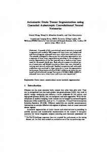
Fig. 1. Frequency Clustering Feature Extraction System Block Diagram.

Due to the standard windowing technique for PSD estimation and smoothness of expected PSD activity across frequency, it is expected that the optimal task-relevant frequency bands will consist of compactly connected neighboring frequency intervals (determined by the frequency resolution of the PSD). The beginning and endpoint of each band, however, must be determined adaptively by investigating the statistical similarity between the frequency intervals that will be potentially integrated in the same frequency band. Note that intuitively, we should cluster together only the frequency intervals that carry statistically similar information. This will increase the signal-to-noise ratio of the generated feature after integration of PSD over the band and will potentially improve classification accuracy. Consequently, we first need to measure how statistically similar two frequency intervals are. The simplest such measure in statistics is the correlation coefficient between them. For the rest of the paper, we will assume that the frequency resolution is 1Hz, thus each frequency interval will be represented by the integer frequency value that the interval is centered at. If two integer frequency components are highly correlated, then they carry redundant information and the combined information is little more than each individual frequency. Thus, combining these correlated frequency components together (for example by averaging, which is what integration does essentially) instead of using them as separate features, will reduce feature dimensionality without sacrificing significant amounts of novel information. In the finite training data case, the generalization benefits one would obtain through reduction in dimensionality will typically surpass the losses incurred due to eliminated information. A more general measure of similarity would be mutual information between pairs of frequencies, however, upon inspection, the authors have determined that the pairwise mutual information (estimated nonparametrically using kernel density estimation) and correlation coefficient matrices for our particular experimental datasets revealed similar clustering structures. Therefore, for the rest of the paper, we focus on correlation coefficients as the primary similarity measure, and adaptively identify the most coherent frequency bands by clustering. The mathematical motivation for the use of correlation coefficient

Fig. 2. A typical correlation matrix for one EEG channel

will be detailed in the next section. II. METHOD The EEG measurements are collected using wireless EEG cap as the subjects are engaged in various mental tasks with different difficulty levels (we will describe the details in section III). Our goal is to design a classification system that can discriminate between various existing tasks and their difficulty levels using the EEG measurements. The block diagram of the designed system that incorporates the proposed automatic frequency band segmentation method is shown in Fig. 1. After preprocessing, including filtering and artifact removal, we get clean multi-channel EEG signals. The integer PSD frequency components are estimated using the Welch method [6] from 1 to 40 Hz. We measure the distance between pairwise frequency components using the correlation coefficient matrix. Given the PSD E(f) at each integer frequency f from 1 to 40 Hz, we construct the frequency-correlation matrix C: L L⎤ ⎡L ⎢ (1) C = ⎢L C (i, j ) L⎥⎥ ⎥ ⎢⎣L L L⎦ Each element of C is the absolute correlation coefficient between E(i) and E(j): | E[( E (i ) − µ i )( E ( j ) − µ j )] | (2) C (i, j ) = Std [ E (i)] ⋅ Std [ E ( j )] where µi denotes E[E(i)]. If the correlations between pairwise frequency components are very strong (close to 1) or very weak (close to 0), then the correlation matrix C approximately becomes block-diagonal. A typical correlation matrix for one EEG channel is shown in Fig. 2. Once we obtain the correlation matrix, we can employ similarity-based clustering algorithms on this matrix to automatically segment the frequency bands. Many existing spectral clustering algorithms can achieve this goal [9-12]. Spectral clustering algorithms in the literature typically deal with similarity matrices formed between pairs of data samples

and for large data sets with N samples, the similarity matrix becomes N×N. Note that the matrix is essentially a fully connected weighted graph between the nodes (the samples in spectral clustering or frequencies in our case). Therefore, the procedure of cutting the weakest connection and then searching for the remaining connected components is not feasible for very large N. In our application, however, the size of the correlation matrix, determined by the frequency resolution of the PSD estimator, is quite small; therefore, we opt for this straightforward procedure and employ the well known connected component search algorithm [13]. Suppose that, after clustering, we get a group of frequencies ⎯ f1, f2, …, fl ⎯ which have strong correlation. Following the typical assumption of a linear generative model for the EEG measurements at each electrode, we can consider specific frequencies to correspond to a certain brain signature, a common source denoted as g. Consequently, this underlying common feature is assumed to take various realizations at each frequency as follows: g ( f i ) = g + n( f i ) (3) where n(fi) is background and measurement noise. Note that this is a simplified linear model and more elaborate linear or nonlinear generative mechanisms will be assumed and tested in future work. Given the model in (3), the common source is extracted by an appropriate weighted average scheme: l

g ≈ ∑ wi g ( f i )

(4)

i =1

to maximize classification performance. For simplicity, we select wi=1/l and observe this value to work well in practice. However, in general optimization of these parameters could be necessary. Based on the model in (3), we can see that the weighted average feature g improves the signal-to-noise ratio, thus resulting in a better feature. The frequency clustering feature extraction method is summarized below: 1. 2. 3.

4.

Estimate PSD at integer frequencies from artifact-free EEG. For each EEG channel, calculate the correlation matrix using equations (1) and (2). For each channel, find a threshold such that when all entries of C below the threshold are zeroed, the connected components algorithm yields a predetermined K number of clusters. Integrate signal power in each frequency band as in (4) determined for each channel to obtain the reduced feature set.

III. EXPERIMENTS AND RESULTS A. Playing a Video Game We applied the proposed automatic frequency band segmentation method to EEG data collected using a wireless EEG cap manufactured by Advanced Brain Monitoring (ABM) [14] with 6 channels: C3, CzPO, F3, FzPO, P4, POz. In the experiments, the subjects are asked to play a video game with varying difficult levels, which correspond to the high and low workloads. EEG signals were collected from 5 subjects and each subject performed 2 sessions. The sampling rate of the EEG is 256Hz. The PSD estimates are offered by

the ABM system using the Welch sliding window (which also includes bandpass and adaptive filtering for noise and artifact removal). A frequency resolution of 1Hz is assumed for the PSD, so energy estimates in 1Hz frequency bins centered at integer frequencies from 1Hz to 40Hz are obtained. The optimal number of frequency clusters for each EEG channel is acquired by cross-validation procedure. Data from each session is partitioned into 5 pieces for 5-fold cross-validation. We employ a Gaussian Mixture Model (GMM) based classifier that generates cognitive load estimates at 10Hz. These estimates are passed through a 2-second-long causal median filter to eliminate occasional outliers and to obtain a smooth cognitive state estimation sequence. The average and standard deviation of correct classification probability is used as the cross-validation measure for order selection in identifying the number of frequency bands. Ideally, one should employ cross-validation to select the number of clusters for each EEG channel as well as the model order for the GMM classifier. For a C-channel EEG recording if we evaluate K different frequency cluster models (that is for each channel evaluate the performance of 1 to K clusters) and M different GMM orders (1 to M Gaussian components), the computational complexity of the cross-validation becomes KCMN. The factor N is the number of random initializations of the EM algorithm to find the global optimum for GMM training. As this complexity tends to increase quite fast, we simplify the search by assuming a predetermined order (M=4) for the GMM classifiers, based on our previous experience with datasets collected using this equipment in similar experimental setups. We also assume that each EEG channel uses the same number of frequency bands, thus the power-dependency in C is eliminated. The computational complexity then reduces to KN 5-fold cross-validation procedures. The overall experimental procedure is: 1) For each session of data, select a random 5-fold partition. 2) Pick 4 for training (TRAIN) and 1 for testing (TEST) 3) For K from 2 to 8 perform the following: - Obtain the reduced dimension features corresponding to the K clusters determined by the segmentation algorithm. - On the reduced dimension features, train 100 randomly initialized GMM classifiers. - Pick the GMM that maximizes the classification

performance on TRAIN. 4) Go to step 2 and repeat until all partitions are used as TEST. 5) Calculate the average and standard deviation of classification error on TEST for the 5 partitions for each K using the best GMMs. 8) Repeat steps 2 to 5 for each session.

The features obtained by automatic segmentation of frequency bands are compared to features obtained by selecting 5 frequency bands in accordance with the clinical and cognitive science literature. These predetermined frequency bands are 1-3Hz, 4-7Hz, 8-12Hz, 13-30Hz, 31-40Hz. The PSD features are extracted by integrating over these frequency bands, which generate 5 features for each

1 0.9

DATA SESSIONS

0.8

0.8

0.7

0.7

EEG channel. The classifiers are trained on these features using Monte Carlo initialization and the best performing classifiers are selected in the 5-fold cross-validation scheme. The mean and standard deviation of correct classification rate for each session for different number of clusters per channel are listed in Table 1. The performance comparison between automatic frequency clustering and manually predefined frequency bands is shown in Fig. 3. Experimental results in Table 1 and Fig. 3 show that in 8 of 10 sessions, the proposed feature extraction method outperforms the previously used predefined frequency bands for the proper number of clusters that one would select in cross-validation. B. Benchmark Mental Task In this experiment, EEG data was collected using a Biosemi Active Two system [18] while 3 subjects executed the Larson task [19]. In the Larson task, the subjects are required to maintain a mental count according to the presented configuration of images on the monitor. The combination of mental activities during this task includes Attention, Encoding, Rehearsal, Retrieval, and Match. The complexity of the task is divided into two classes, low and

0.5 0.4

0.5 0.4

0.2

frequency clustering manually defined

0.1 0 0

0.6

0.3

0.2

1

2

3

4 5 number of clusters

6

7

8


0.1 0 0

9

1

2

0.9

0.9

0.8

0.8

0.7

0.7

0.6 0.5 0.4 0.3

8

9


0.5 0.4

1

2

3


6

7

8

0.1 0 0

9

1

2

(Session 3)

3


6

7

8

9

(Session 4)

0.9

0.9

0.8

0.8

0.7

0.7 classification rate

1

0.6 0.5 0.4 0.3


0.6 0.5 0.4 0.3

0.2

0.2


0.1

1

2

3


6

7

8

0.1 0 0

9

1

2

(Session 5)

3


6

7

8

9

(Session 6)

1

1 frequency clustering manually defined

0.9


0.9 0.8

0.7


0.8

0.6 0.5 0.4

0.6 0.5 0.4

0.3

0.3

0.2

0.2

0.1

0.1

1

2

3


6

7

8

0 0

9

1

2

(Session 7)

3


6

7

8

9

(Session 8)

1

1 frequency clustering manually defined

0.9


0.9

0.8

0.8

0.7

0.7

0.6 0.5 0.4

0.6 0.5 0.4

0.3

0.3

0.2

0.2

0.1 0 0

7

0.6

1

0 0

6

0.2


0.1

0 0


0.3

0.2

0 0

3

(Session 2) 1

classification rate

classification rate

(Session 1) 1

classification rate

The second column presents the results for manually predefined frequency bands; columns 3 to 9 correspond to K equals 2 to 8 automatically determined frequency bands. The results are shown in the form mean+/-std.

0.6

0.3

classification rate

8 0.75 +/0.23 0.65 +/0.11 0.62 +/0.07 0.46 +/0.11 0.62 +/0.04 0.45 +/0.06 0.53 +/0.12 0.47 +/0.08 0.58 +/0.09 0.59 +/0.07

classification rate

2 0.79 +/0.13 0.70 +/0.16 0.66 +/0.11 0.54 +/0.10 0.60 +/0.13 0.53 +/0.10 0.60 +/0.06 0.46 +/0.11 0.56 +/0.04 0.60 +/0.13

classification rate

Manual 0.78 Session +/1 0.21 0.74 Session +/2 0.18 0.61 Session +/3 0.13 0.53 Session +/4 0.09 0.62 Session +/5 0.11 0.46 Session +/6 0.05 0.60 Session +/7 0.10 0.52 Session +/8 0.07 0.56 Session +/9 0.07 0.64 Session +/10 0.09

Number of clusters per EEG channels 3 4 5 6 7 0.79 0.70 0.75 0.74 0.74 +/+/+/+/+/0.18 0.19 0.18 0.15 0.22 0.71 0.68 0.66 0.69 0.69 +/+/+/+/+/0.09 0.20 0.16 0.15 0.16 0.66 0.71 0.60 0.63 0.65 +/+/+/+/+/0.05 0.10 0.11 0.10 0.11 0.51 0.56 0.62 0.53 0.49 +/+/+/+/+/0.12 0.12 0.15 0.08 0.12 0.63 0.60 0.58 0.59 0.64 +/+/+/+/+/0.12 0.09 0.05 0.06 0.05 0.48 0.52 0.49 0.48 0.53 +/+/+/+/+/0.09 0.07 0.11 0.10 0.09 0.5i 0.62 0.58 0.55 0.57 +/+/+/+/+/0.06 0.15 0.10 0.07 0.10 0.52 0.59 0.61 0.55 0.45 +/+/+/+/+/0.16 0.06 0.12 0.08 0.12 0.54 0.52 0.53 0.59 0.59 +/+/+/+/+/0.07 0.07 0.09 0.09 0.07 0.58 0.57 0.58 0.58 0.62 +/+/+/+/+/0.10 0.08 0.13 0.07 0.10

classification rate

1 0.9

classification rate

TABLE I MEAN AND STANDARD DEVIATION OF CLASSIFICATION RATE FOR DIFFERENT

0.1

1

2

3


6

7

8

9

0 0

1

2

3


6

7

8

9

(Session 9) (Session 10) Fig. 3. Performance comparison between automatic frequency band segmentation (for 2 to 8 bands) and manually predefined frequency bands in terms of correct classification probability (between 2 classes). The latter is depicted as a separate error bar located at x-axis value of 1.

high workloads, which depend on the inter-stimuli interval. The Biosemi system uses a 30 channel EEG cap and eye electrodes. Vertical and horizontal eye movements and blinks were recorded with electrodes below and lateral to the left eye. EEG is sampled and recorded at 256Hz from 30 channels.

TABLE II MEAN AND STANDARD DEVIATION OF CLASSIFICATION RATE FOR DIFFERENT

1 0.9

SUBJECTS IN LARSON TASK

2 0.96 +/0.01 0.88 +/0.15 0.65 +/0.12

Number of clusters per EEG channels 3 4 5 6 7 0.96 0.77 0.87 0.67 0.5 +/+/+/+/+/0 0.02 0.22 0.11 0.08 0.86 0.85 0.88 0.68 0.57 +/+/+/+/+/0.13 0.11 0.06 0.04 0.15 0.63 0.67 0.56 0.54 0.49 +/+/+/+/+/0.08 0.09 0.10 0.06 0.05

0.8

8 0.5 +/0 0.63 +/0.12 0.53 +/0.09


Manual Subject 0.91 1 +/0.04 Subject 0.80 2 +/0.06 Subject 0.63 3 +/0.15

0.6 0.5 0.4 0.3 0.2


0.1 0

0

1

2

3


6

7

8

9

(Subject 1)

The second column presents the results for manually predefined frequency bands; columns 3 to 9 correspond to K equals 2 to 8 automatically determined frequency bands. The results are shown in the form mean+/-std.

1 0.9 0.8

EEG signals are preprocessed to remove eye blinks using an adaptive linear filter based on the Widrow-Hoff training rule (LMS) [20]. Information from the VEOGLB ocular reference channel was used as the noise reference source for the adaptive ocular filter. DC drifts were removed using high pass filters (0.5Hz cut-off). A band pass filter (2Hz-50Hz) was also employed, as this interval is generally associated with cognitive activity. The PSD was estimated for integral frequency from 1 to 40 Hz using Welch method [6]. We repeat the same procedure described in the previous experiment. The mean and standard deviation of correct classification rate for each subject for different number of clusters per channel are listed in Table 2. The performance comparison between automatic frequency clustering and manually predefined frequency bands is shown in Fig. 4. Experimental results in Table 2 and Fig. 4 show that for the Larson task, the proposed feature extraction method outperforms the previously used predefined frequency bands for all subjects.

classification rate

0.7 0.6 0.5 0.4 0.3 0.2


0.1 0

0

1

2

3


6

7

8

9

(Subject 2) 1 frequency clustering manually defined

0.9 0.8

classification rate

0.7 0.6 0.5 0.4 0.3 0.2 0.1

IV. CONCLUSION In this paper, we proposed a feature dimensionality reduction method for BCI systems utilizing PSD features. The method is evaluated on EEG data collected in the AugCog context. Although we have focused on the specific application and feature set, the principle of reducing the feature dimensionality through automatic clustering based on statistical similarity can be applied to arbitrary feature sets in any classification problem. With suitable pairwise similarity metrics, the method is expected to provide a practically feasible alternative to feature selection and projection techniques that rely on high dimensional statistical quantities, which require an exponentially growing number of samples for accurate estimation. In future work, we will investigate more elaborate generative models for highly correlated pair of features (such as arbitrary nonlinear dependencies) and employ higher order statistical measures (such as mutual information) to determine semi-independent clusters of features. The procedure will also be tested on benchmark pattern

0

0

1

2

3


6

7

8

9

(Subject 3) Fig. 4. Performance comparison between automatic frequency band segmentation (for 2 to 8 bands) and manually predefined frequency bands in terms of correct classification probability (between 2 classes). The latter is depicted as a separate error bar located at x-axis value of 1.

recognition datasets. ACKNOWLEDGMENT This work was supported by DARPA under contract DAAD-16-03-C-0054 and by NSF under grant ECS-0524835. The EEG data was collected at the Human-Centered Systems Laboratory, Honeywell, Minneapolis, Minnesota. REFERENCES [1]

T. Lan, D. Erdogmus, A. Adami, M. Pavel, S. Mathan, “Salient EEG Channel Selection in Brain Computer Interfaces by Mutual Information Maximization,” Proceedings of EMBC’05, 2005.

[2]

[3] [4]

[5]

[6]

[7]

[8]

[9]

[10]

[11]

[12] [13] [14] [15]

[16] [17]

[18] [19]

[20]

T. Lan, D. Erdogmus, A. Adami, M. Pavel, “Feature Selection by Independent Component Analysis and Mutual Information Maximization in EEG Signal Classification,” Proceedings of IJCNN’05, pp. 3011-3016, 2005. T. Lan, A. Adami, D. Erdogmus, M. Pavel, “Estimating Cognitive State Using EEG Signals,” Proceedings of EUSIPCO’05, 2005. J.R. Wolpaw, N. Birbaumer, D.J. McFarland, G. Pfurtscheller, T.M. Vaughan, “Brain–Computer Interfaces for Communication and Control,” Clinical Neurophysiology, vol. 113, pp. 767-791, 2002. K-R. Muller, M. Krauledat, G. Dornhege, G. Curio, B. Blankertz, “Machine Learning Techniques For Brain-Computer Interfaces. Biomedical Engineering,” vol. 49, no. Sup. 1, pp. 11-22, 2004. P. Welch, “The Use of Fast Fourier Transform for the Estimation of Power Spectra: A Method Based on Time Averaging Over Short Modified Periodograms”, IEEE Transactions on Audio and Electroacoustics, vol. 15, no. 2, pp. 70-73, 1967. A. Gevins, M.E. Smith, L.McEvoy, D. Yu, “High Resolution EEG Mapping of Cortical Activation Related to Working Memory: Effects of Task Difficulty, Type of Processing, and Practice,” Cerebral Cortex, vol. 7, pp. 374-385, 1997. M. Pregenzer, G. Pfurtscheller, “Frequency Component Selection for an EEG-Based Brain to Computer Interface,” IEEE Transactions on Rehabilitation Engineering, vol. 7, no. 4, 1999. H. Zha, C. Ding, M. Gu, X. He, and H.D. Simon. Spectral relaxation for K-means clustering. Advances in Neural Information Processing Systems 14 (NIPS 2001). pp. 1057-1064, Vancouver, Canada. Dec. 2001. L. Hagen and A.B. Kahng. New spectral methods for ratio cut partitioning and clustering. IEEE. Trans. on Computed Aided Desgin, 11:1074--1085, 1992. M. Belkin and P. Niyogi. Laplacian Eigenmaps and Spectral Techniques for Embedding and Clustering, Advances in Neural Information Processing Systems 14 (NIPS 2001), pp: 585-591, MIT Press, Cambridge, 2002. F.R. Bach and M.I. Jordan. Learning spectral clustering. Neural Info. Processing Systems 16 (NIPS 2003), 2003. T.H. Cormen, C.E. Leiserson, R.L. Rivest, “Introduction to Algorithms,” MIT Press, pp. 441, 1990. http://www.b-alert.com/EEG.html A.P. Dempster, N.M. Laird, D.B. Rubin, “Maximum Likelihood from Incomplete Data via the EM Algorithm,” Journal of the Royal Statistical Society, vol. 39, pp. 1-38, 1977. R.O. Duda, P.E. Hart, D.G. Stork, Pattern Classification, 2nd ed., Wiley, 2000. E. Parzen, “On Estimation of a Probability Density Function and Mode”, in Time Series Analysis Papers, Holden-Day, Inc., San Diego, California, 1967. http://www.biosemi.com E. Halgren, C. Boujon, J. Clarke, C. Wang, and P. Chauvel, Rapid Distributed Fronto-parieto-occipital Processing Stages During Working Memory in Humans. Cerebral Cortex, Vol. 12, No. 7, Jul. 2002. B. Widrow and M. E. Hoff, “Adaptive Switching Circuits,” in IRE WESCON convention Record, 1960, pp. 96-104.