Time-Frequency Sparseness in the Presence of. Spatial Aliasing. Benedikt Loesch and Bin Yang. Chair of System Theory and Signal Processing, University of ...
Blind Source Separation based on Time-Frequency Sparseness in the Presence of Spatial Aliasing Benedikt Loesch and Bin Yang Chair of System Theory and Signal Processing, University of Stuttgart {benedikt.loesch, bin.yang}@LSS.uni-stuttgart.de
Abstract. In this paper, we propose a novel method for blind source separation (BSS) based on time-frequency sparseness (TF) that can estimate the number of sources and time-frequency masks, even if the spatial aliasing problem exists. Many previous approaches, such as degenerate unmixing estimation technique (DUET) or observation vector clustering (OVC), are limited to microphone arrays of small spatial extent to avoid spatial aliasing. We develop an offline and an online algorithm that can both deal with spatial aliasing by directly comparing observed and model phase differences using a distance metric that incorporates the phase indeterminacy of 2π and considering all frequency bins simultaneously. Separation is achieved using a linear blind beamformer approach, hence musical noise common to binary masking is avoided. Furthermore, the offline algorithm can estimate the number of sources. Both algorithms are evaluated in simulations and real-world scenarios and show good separation performance. Key words: blind source separation, adaptive beamforming, spatial aliasing, time-frequency sparseness
1
Introduction
The task of convolutive blind source separation is to separate M convolutive mixtures xm [i], m = 1, . . . , M into N different source signals. Mathematically, we write the sensor signals xm [i] as a sum of convolved source signals N X xm [i] = hmn [i] ∗ sn [i], m = 1 . . . M (1) n=1
Our goal is to find signals yn [i], n = 1 . . . N such that, after solving the permutation ambiguity, yn [i] ≈ sn [i] or a filtered version of sn [i]. In the case of moving sources, the impulse responses hmn [i] are time-varying. ¯ l] in the time-frequency Our algorithms cluster normalized phase vectors X[k, domain, where k is the frequency index and l is the time frame index, respectively. Each cluster with the associated state vector c[k, pn ] corresponds to a different source n with the associated location or direction-of-arrival (DOA) parameter vector pn . Different from DUET, our algorithms can use more than
2
Benedikt Loesch and Bin Yang
two microphones. In contrast to DUET and OVC, our algorithms do not suffer ¯ l], we from the spatial aliasing problem. After clustering the phase vectors X[k, apply time-frequency masking or the blind beamformer from [1] to separate the sources.
2
Proposed Offline Algorithm
After a short-time Fourier transform (STFT), we can approximate the convolutive mixtures in the time-domain as instantaneous mixtures at each timefrequency (TF) point [k, l]: N X X[k, l] ≈ Hn [k]Sn [k, l] (2) n=1
X = [X1 , . . . , XM ]T is called an observation vector and Hn = [H1n , . . . , HMn ]T is the vector of frequency responses from source n to all sensors. We assume that the direct path is stronger than the multipath components. This allows us to exploit the DOA information to perform the separation. Note that we are only interested in separation and not in dereverberation. Hence, we do not aim at a complete inversion of the mixing process. As a consequence, we do not require minimum-phase mixing. The proposed algorithm consists of three steps: normalization, clustering, and reconstruction of the separated signals. 2.1
Normalization
From the observation vectors X[k, l], we derive the normalized phase vectors ¯ l] which contain only the phase differences of the elements of X[k, l] with X[k, respect to a reference microphone J: i h ¯ l] = ej·arg(Xm [k,l]/XJ [k,l]) , m = 1, · · · , M (3) X[k, For a single active source, the phase of the ratio of two elements of X[k, l] is a linear function of the frequency index k (modulo 2π): arg (Xm [k, l]/XJ [k, l]) = 2π∆f kτm + 2πo,
o∈Z
(4)
where ∆f is the frequency bin width and τm is the time-difference of arrival (TDOA) of the source with respect to microphone m and J. If there is no spatial aliasing (i.e.ho = 0), iwe can cluster the TDOAs at all TF points because of τm =
1 2π∆f k
arg
Xm [k,l] XJ [k,l]
. However, in the case of spatial aliasing (o 6= 0), i h Xm [k,l] 1 we can no longer cluster 2π∆f arg k XJ [k,l] directly. Instead we would need to take into account all possible values of o. However, we can avoid this problem by directly comparing the observed phase difference and the model phase difference for multiple microphone pairs using the distance metric � � � � M X Xm [k, l] 2 ¯ kX[k, l] − c[k, p]k = 2M − 2 · cos arg − 2π∆f kτm (p) (5) XJ [k, l] m=1
TF Sparseness based BSS in the Presence of Spatial Aliasing
3
� � with the state vector c[k, p] = [cm ]1≤m≤M = ej2π∆f kτm (p) 1≤m≤M . c[k, p] contains the expected phase differences for a potential source at p with respect to microphones m = 1, · · · , M and J. The distance metric (5) allows an estimation of the location or DOA parameters pn of all sources even if spatial aliasing occurs. This is achieved by considering all frequency bins simultaneously: Due to the spatial aliasing, (5) contains location ambiguities for higher frequencies. However, these ambiguities are removed by summing across all frequency bins. We define J (p) X X ¯ l] − c[k, p]k2 ), J (p) = Jl (p) = ρ(kX[k, Jl (p), (6) k
l
which has maxima for p = pn . ρ(t) is a monotoneously decreasing nonlinear function in the range [0, 1] that reduces the influence of outliers and increases spatial resolution. We estimate pn by looking for the maxima of J (p) and then cluster the TF points as described in the next section. 2.2
Source Number Estimation and Clustering
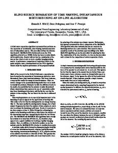
ˆ and then find clusters C1 , . . . , C ˆ We need to estimate the number of sources N N ¯ ˆ n ]. Unlike [2–4], we achieve the clustering by a of X[k, l] with centroids c[k, p direct search over all possible TDOAs or DOAs p and do not use iterative approaches such as k-means or expectation-maximization (EM). This has the advantage, that we are guaranteed to find the global optima √ of the cost function. Inspired from [5], we propose to use ρ(t) = 1 − tanh(α t) as the nonlinear function ρ(t) in (6). Independently of our research, [6] proposed a similar cost function Jl for only two microphones and without the summation over time for localization purposes. Another advantage of the direct search is that we do not need to know the number of sources beforehand as in [2]. Instead, we can count the number of significant and distinct peaks of J (p): This is done by finding all peaks pn of J (p) with J (p) > t and sorting the peaks in descending order J (pi ) > J (pi+1 ). Then we start from the first peak and accept the next peak if the minimum distance to a previously accepted peak is larger than a certain threshold t2 . The ˆ is then given as the number of accepted peaks. number of estimated sources N Since in (6) the peak height is a function of the amount of source activity it might be difficult to count the number of sources if the amount of source activity differs a lot among the sources. One way to solve this problem is to use the max-approach from [6] to estimate the number of sources by replacing J (p) by J˜(p) = maxl Jl (p). This modified function is less sensitive to the amount of source activity because the peak height is proportional to the coherence of the observed phase. So if for each source there is at least one time frame where it is the single active source, J˜(p) will yield a large peak for this source. Fig. 1 shows J (p) and J˜(p) for two scenarios with different amounts of source activity. In Fig. 1(b) the max-approach is clearly superior because the contrast beetween true
4
Benedikt Loesch and Bin Yang
peaks and spurious peaks is larger. Furthermore, the max-approach improves TDOA estimation for closely spaced microphones: It selects time frames with high coherence of the observed phase, i.e. a single active source.
1
1 J (p) J˜(p)
0.8 0.6
0.6
0.4
0.4
0.2
0.2
0 0
100
200 θ [°]
300
(a) Sources always active
J (p) J˜(p)
0.8
400
0 0
100
200 θ [°]
300
400
(b) Src 3: start 10 s, Src 4: start 14 s
Fig. 1. Source Number and DOA Estimation for different source acitivity (length 24 s)
ˆ of the sources are given by the relevant ˆ n , n = 1, · · · , N The positions/DOAs p ˜ peaks of J (p) or J (p). For each source, we generate the corresponding state ˆ and assign all TF points to cluster n for which ˆ n ], n = 1, · · · , N vectors c[k, p 2 ¯ ˆ n ]k is minimal. kX[k, l] − c[k, p Comparison with EM algorithm with GMM model : [4] uses a related approach for two microphones: They use an EM algorithm with a Gaussian mixture model (GMM) for the phase difference between the two microphones at each TF point. The phase difference of each source is modelled as a mixture of 2Kf + 1 Gaussians with mean 2πk · (1 + ∆f µq ), k = −Kf , · · · , Kf , where µq is the mean of the q-th component. The observed phase difference for all sources is then described as a mixture of Q such models. Furthermore they use a Dirichlet prior for the mixture weights αq , q = 1, · · · , Q to model the sparsity of the source directions, i.e. to represent the phase difference with a small number of Gaussians with large weight αq . After convergence of the EM algorithm the mean µq of the Gaussians with large weight αq and small variance σq2 reflect the estimated TDOAs of the N sources. Our approach differs in a number of ways: – We use a direct search instead of an iterative procedure to estimate the source parameters pn . – We are guaranteed to find the global optima of the function J (p), whereas the EM algorithm could converge to local optima. – We estimate the number of sources by counting the number of significant and distinct peaks instead of checking the weights and variance of the components of a GMM model. – We do not model the phase difference of each source using 2Kf + 1 Gaussians. Instead we use the distance metric (5) which incorporates the phase wrapping.
TF Sparseness based BSS in the Presence of Spatial Aliasing
5
– Our approach is computationally less demanding: We need Ngrid · K · L function evaluations, while the EM algorithm requires Niter ·Q·(2Kf +1)·K ·L function evaluations. For a typical scenario Ngrid = 180, Niter = 10, Q = 8, Kf = 5 and assuming comparable computational cost for each function evaluation, our approach would be about 6 times faster. The differences between [4] and our approach can be summarized as differences in the model (wrapped Gaussians vs. 2π-periodic distance function) and in the clustering algorithm (iterative EM algorithm vs. direct search and simple clustering). The authors would like to thank Dr. Shoko Araki for running our proposed algorithm on her dataset from [4]. Using t = 0.5 and t2 = 5◦ , our algorithm estimates the number of sources correctly for all tested cases. 2.3
Reconstruction
To reconstruct the separated signals, we use the blind beamforming approach discussed in [1]. This approach reduces or completely removes musical noise artifacts which are common in binary TF mask based separation. After the beamforming step, additional optional binary TF masks can be used to further suppress the interference. Then we convert the separated signals back to the time domain using an inverse STFT.
3
Online Separation Algorithm
The online algorithm operates on a single frame basis and uses a gradient ascent search for the TDOAs/DOAs of the sources with prespecified maximum number of sources N . Inactive sources result in empty clusters. The cost function Jl for the l-th STFT frame is X ¯ l] − c[k, pn ]k2 ) Jl (pn ) = ρ(kX[k, (7) k
Its gradient vector with respect to pn is � X � ∂ρ(t) ∂ττ ∂Jl ¯ =− · c[k, pn ] ⊙ 2(X[k, l] − c[k, pn ]) , (8) · ℜ j2π∆f k · ∂pn ∂t ∂pn k
where τ = [τm ]1≤m≤M . Similar to [7], we use a time-varying learning rate which is a function of the amount of TF points associated with source n. The separation steps are similar to the offline algorithm. A computationally efficient version of the blind beamforming algorithm can be obtained by using recursive updates of the parameters as in [8].
4
Experimental Evaluation
For the experimental evaluation, we used a sampling frequency of fs = 16 kHz, a STFT with frame length 1024 and 75% overlap. SNR was set to 40 dB. We selected six speech signals from the short stories of the CHAINS corpus [9].
6
4.1
Benedikt Loesch and Bin Yang
Stationary Sources
First, we evaluate the offline algorithm using the measured impulse responses of room E2A (T60 = 300 ms) from the RWCP sound scene database [10]. This database contains impulse responses for sources located on a circle with radius 2.02 m with an angular spacing of 20◦ . The microphone array is shifted by 0.42 m with respect to the center of the circle. We consider a two-microphone array with the spacings d = 11.3 cm and d = 33.9 cm. All sources have equal power and a length of 5 s. For d = 11.3 cm, J (p) sometimes does not show N distinct maxima. Hence, we use J˜(p) for d = 11.3 cm since it provides increased resolution by using frames with a single active source for the localization. We have tried different signal combinations and DOA scenarios (A,B,C,D): For scenarios A,B,C we varied the DOAs between 30◦ . . . 150◦ and tested different angular spacings between the sources. For case D we distributed the sources with maximum angular spacing between 10◦ . . . 170◦ . The angular spacings between the sources are summarized in Table 1. For each scenario, we considered all signal combinations Table 1. Considered scenarios A B C D N =2 20◦ – 40◦ 160◦ N =3 20◦ /40◦ 40◦ /20◦ 40◦ /40◦ 80◦ /80◦ N = 4 20◦ /40◦ /40◦ 40◦ /20◦ /40◦ 40◦ /40◦ /40◦ 60◦ /40◦ /60◦
of N = 2, 3, 4 out of the 6 source signals. Table 2 summarizes the performance of the source number estimation and the signal-to-interference (SIR) gain for the different cases. For the source number estimation, we used thresholds t = 0.46 for d = 11.3 cm and t = 0.55 for d = 33.9 cm. t2 was set to 10◦ for both microphone spacings d. The performance is evaluated by the percentage of estimations for ˆ = n, n = 1, · · · , 5. This is known as the confusion matrix. which N Table 2. Source number estimation and SIR gain
N spacing d = 11.3 cm 2 d = 33.9 cm d = 11.3 cm 3 d = 33.9 cm d = 11.3 cm 4 d = 33.9 cm
1 0 0 0 0 0 0
ˆ accuracy (%) N 2 3 4 97 3 0 100 0 0 1 98 1 0 100 0 0 2 95 0 0 100
5 0 0 0 0 3 0
SIR gain [dB] A B C D 4.6 – 7.9 15.9 6.0 – 9.0 13.0 3.7 5.7 8.7 11.4 6.2 8.9 9.4 13.1 2.8 6.0 7.1 6.4 6.5 8.9 8.0 8.4
Our offline algorithm estimates the number of sources correctly in almost all cases and shows a good separation performance. A larger microphone spacing
TF Sparseness based BSS in the Presence of Spatial Aliasing
7
achieves a better separation performance for closely spaced sources (case A and B) or for large source numbers. On the short two-source-two-microphone mixtures of the SISEC2010 campaign (http://irisa.fr/metiss/SiSEC10/short/ short_all.html), separation performance is comparable to other algorithms. 4.2
Moving Sources
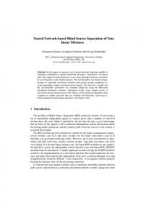
In order to have a precise reference for moving source positions, we performed simulations using the MATLAB ISM RoomSim toolbox [11]. The considered room was of size 5 m × 6 m × 2.5 m and we chose reverberation times of T60 = 100, 200, 300 ms. We used a cross-array ( ) with M = 5 microphones. The microphone spacing was d = 10 cm, so spatial aliasing occurs above 1700 Hz . We have N = 3 sources that move along a circle with radius 1.0 m. Source 1 moves from θ1 = 30◦ to θ1 = 120◦ and back, source 2 moves from θ2 = 120◦ to θ2 = 210◦ and back and source 3 moves from θ3 = 240◦ to θ3 = 300◦. The total simulation time is 24 s. Fig. 2(a) shows the estimated angles θˆonl [l] using our online algorithm as well as the reference angles θtrue [l]. The online-algorithm was initialized with the true angles θtrue [0]. As we see, the online algorithm accurately tracks the sources. During speech pauses, angle estimates are not updated. The separation performance of the online and offline algorithm is summarized in Table 3. As expected, the offline algorithm fails to separate the source signals while our gradient-based online algorithm achieves good results. The reason for the failure of the offline algorithm is that it averages the DOAs of the moving sources. The estimated DOAs are 63◦ , 119◦ and 240◦ . Two of the three estimated DOAs match the initial and final DOAs of the two sources and hence separation quality for these two sources (2 and 3) is acceptable for T60 = 100 ms. However, the separation performance drops significantly when the sources start moving as shown in Fig. 2(b). It shows the local SIR gains which are calculated over non-overlapping segments of 1 second and averaged over the three sources. Table 3. Global SIR gain in dB for moving sources algorithm source 1 source 2 source 3 mean offline 4.5 18.2 10.1 10.9 100 ms online 25.9 28.1 27.8 27.3 offline 5.0 15.9 8.5 9.8 200 ms online 24.6 22.4 24.1 23.7 offline 4.9 10.7 6.9 7.5 300 ms online 17.3 16.5 18.0 17.3 T60
5
Conclusion
In this paper we have presented two blind source separation algorithms based on TF sparseness that are able to deal with the spatial aliasing problem by using
Benedikt Loesch and Bin Yang 350 300 angle [°]
250
ˆ θ onl θtrue
30 SIR gain [dB]
8
200 150 100 50 0 0
20 10 0 −10
5
10
15 time [s]
(a) DOA tracking
20
25
0
online offline 5
10
15
20
25
time [s]
(b) Local SIR gain
Fig. 2. Fixed number of moving sources, T60 = 200 ms
a distance metric which incorporates phase wrapping (mod 2π) and averaging all frequency bins for the estimation of the location or DOA parameters of the sources. The offline algorithm reliably estimates the source number and achieves the clustering using a direct search. The online algorithm assumes a prespecified maximum number of sources and is able to track moving sources. Both algorithms show good separation performance in midly reverberant environments.
References 1. J. Cermak, S. Araki, H. Sawada, and S. Makino, “Blind source separation based on a beamformer array and time frequency binary masking,” Proc. ICASSP, 2007. 2. S. Araki, H. Sawada, R. Mukay, and S. Makino, “Underdetermined blind sparse source separation of arbitrarily arranged multiple sensors,” Signal Processing, vol. 87, no. 8, pp. 1833–1847, 2007. 3. H. Sawada, S. Araki, R. Mukay, and S. Makino, “Grouping separated frequency components by estimating propagation model parameters in frequency-domain blind source separation,” IEEE Transactions on Audio, Speech and Language Processing, vol. 15, no. 5, pp. 1592–1604, 2007. 4. S. Araki, T. Nakatani, H. Sawada, and S. Makino, “Stereo source separation and source counting with MAP estimation with Dirichlet prior considering spatial aliasing problem,” Proc. ICA, 2009. 5. F. Nesta, M. Omologo, and P. Svaizer, “A novel robust solution to the permutation problem based on a joint multiple TDOA estimation,” Proc. International Workshop for Acoustic Echo and Noise Control (IWAENC), 2008. 6. Z.E. Chami, A. Guerin, A. Pham, and C. Serviere, “A phase-based dual microphone method to count and locate audio sources in reverberant rooms,” Proc. WASPAA, 2009. 7. S. Rickard, R. Balan, and J. Rosca, “Real-time time-frequency based blind source separation,” Proc. ICA, 2001. 8. B. Loesch and B. Yang, “Online blind source separation based on time-frequency sparseness,” Proc. ICASSP, 2009. 9. F. Cummins, M. Grimaldi, T. Leonard, and J. Simko, “The CHAINS corpus (characterizing individual speakers),” http://chains.ucd.ie/, 2006. 10. Real World Computing Partnership, “RWCP Sound Scene Database in Real Acoustic Environment,” http://tosa.mri.co.jp/sounddb/indexe.htm, 2001. 11. E. Lehmann, “Image-source method for room impulse response simulation (room acoustics),” http://www.watri.org.au/~ ericl/ism_code.html, 2008.