Purdue University
Purdue e-Pubs Computer Science Technical Reports
Department of Computer Science
1992
Boolean Set Operations on a MIMD Distributed Memory Machine Chandrajit L. Bajaj Tamal K. Dey Report Number: 92-079
Bajaj, Chandrajit L. and Dey, Tamal K., "Boolean Set Operations on a MIMD Distributed Memory Machine" (1992). Computer Science Technical Reports. Paper 999. http://docs.lib.purdue.edu/cstech/999
This document has been made available through Purdue e-Pubs, a service of the Purdue University Libraries. Please contact
[email protected] for additional information.
BOOLEAN SET OPERATIONS ON A MIMD DISTRffiUTED MEMORY MACHINE
Chandrajit Bajaj Tarnal Dey
CSD·TR·92-079 October 14, 1992
Boolean Set Operations on a MIMD Distributed Memory Machine* Chandrajit L. Bajaj
Department of Computer Science, Purdue University, West Lafayettte, IN 47907 Tarnal f( Dey Department of Computer and Information Science Indiana-Purdue University at Indianapolis Indianapolis, IN 46202
Abstract We present an efficient algorithm for Boolean Set operations between two arbitrary manifold polyhedra, on a MIMD distributed memory machine such as as the nCUBE2 or the Intel IPSC860. For two manifold polyhedra with O(n) edges each, our algorithms run in 0(log2 n ) time on an n 2 processor MIMD machine. Our model of computation assumes exact arithmetic on each processor and the ability for any processor PI to communicate an 0(1) size message in 0(1) time to any other processor P2 if PI knows P2'S ID. In this paper we also present a distributed data structure for arbitrary polyhedra on MIMD distributed memory machines.
1
Introduction
One way to create a computer solid model of complicated physical object is to express the final solid as the result of (regularized) Boolean set operations on simpler, pre-existing simpler solids, see for example [5,6,7,9,10]. Regularized set operations ensure that the resulting solid is closed and has no boundary points with neighborhoods not intersecting the interior of the solid [9]. In t his paper we consider regularized boolean set operations on arbitrary manifold poly hedra 1 • For polyhedra represented by their boundary elements, the complement set operation of the 'Supported in part by NSF grant CCR 90-02228, NSF grant OMS 91-01424 and AFOSR contract 91-0276 I
Each point of the boundary has a neighborhood that is homeomorphic to an open disk
1
2
l\lIMD DISTRIBUTED MEMORY COMPUTATIONAL MODEL
2
polyhedron (interchange the interior with the exterior) is quite straightforward and amounts to changing the orientation of boundary face cycles. Since all Boolean set operations can be expressed as a combination of complement and intersection operations (DeMorgan 's Laws), it suffices to construct an efficient intersection set operation for two polyhedra. A polyhedron can be represented on a computer by its boundary, i.e., a list of the vertices, edges, and faces of its surface along with numerical and adjacency information for these surface features. Here we propose a distributed boundary representation for polyhedra, a variant of the Star-Edge data structure of [5], for distributed memory multiprocessing machines. In this representation scheme, individual features of the polyhedra are distributed amongst the resident processors in a way that allows one to perform boolean set operations on manifold polyhedra efficiently in a distributed environment. In this paper, the Boolean set operations assume that the input polyhedra conform to this distributed representation and therefore also yield the same distributed boundary representaion for the output polyhedra. Prior work on parallel computational geometry has focussed primarily on shared memory multiprocessing machines [1,3]. For input polyhedra with O( n) edges all of the known algorithms [5,6, 7,9, 10] finds the intersection of two polyhedra in O( n 2 log n) time on a sequential computer. In this paper, we develop a parallel algorithm on a MIMD distributed memory machine to compute the intersections of two manifold polyhedra with O( n) edges. Our algorithm runs in 0(log2 n) time and uses O( n 2 ) processors.
2
MIMD Distributed Memory Computational Model
Each processor is a Random Access Machine with local memory and the ability to perform exact real arithmetic (add, mult, divide etc.) in O( 1) (constant) time.
Each processor PI
can communicate 0 (1) size message in constant time to another processor P2 if Pl knows P2'S ID (Identifying index). Further, a processor can broadcast 0(1) size messages in 0(1) time to other processors. In MIMD architectures such as the hypercube, for the communication between the two cross-diagonal processors (most distant) on a d-dimensional cube one may tag on an additional
o (log d)
factor to the time complexity, however such delays are rarely seen
in practice [8]. For such a computation model, a set of processors each containing O( 1) values
3
DISTRIBUTED BOUNDARY REPRESENTATION
3
sorts them in O(log2 n) time and each processor acquires the ID of the processor containing the next element in the sorted order [2,4].
3
Distributed Boundary Representation
The polyhedra considered in this paper may have voids, several connected components, and their surfaces are manifolds. A polyhedron is represented by a list of its boundary features (faces, edges, and vertices) along with numerical and adjacency information. A directed edge is the description of the incidence of an edge and a face bounded by that edge. The directed edge is oriented in such a way that the face lies to the right of the directed edge when viewed from above the face. Each edge e has two directed edges corresponding to two adjacent faces on which e is lying. These pair of directed edges are called partnered directed edges. We use the following data structure to represent a manifold polyhedron. The top level structure is a collection of faces which are represented by a collection of directed cycles made out of directed edges. Each directed edge points to the next directed edge on its cycle. It also stores the coordinates of the two end points of the corresponding edge and the equation of its face. We use this minimal data structure to compute the polyhedral intersections in distributed environment. Unlike Star-Edge data structure of [5] we do not maintain the information about the nesting of the cycles of a face. The side of the directed edge containing the corresponding face is immediately obtained from its direction. This saves the expensive computation of the nesting structure of a set of cycles on a face and still enables us to detect if we are inside the face as we go along a line from cycle to cycle. Other than this the major difference between this simplified data structure and the Star-Edge data structure is that we do not maintain multiple (more than O( 1)) pointers to a single structure. For example, in Star-Edge data structure, the directed edges maintain a pointer to the corresponding edge which maintain two more pointers for two vertices. This gives multiple pointers to the same vertex. To avoid this the vertices are duplicated with their coordinates for each directed edge. Maintaining multiple pointers to a single structure prohibits the processors to run in parallel whenever they need to access that
4
OVERVIEW OF ALGORITHM
4
single structure simultaneously. In distributed data structure, directed edges are distributed over the processors so that each processor gets 0(1) directed edges. A processor containing a directed edge acquires the ID of the other processor containing the partnered directed edge and also the directed edge ID of the processor containing the next directed edge on the cycle. From this distributed data structure one can obtain the serial version of the simplified data structure in O( n) time and vice versa. The simplified data structure can be converted into Star-Edge data structure in O( n log n) serial time.
4
Overview of algorithm
To understand the partition of the problem, consider the following 2D array. For each face of A, allocate a number of adjacent rows of the array. The number of rows allocated for a face should be the smallest power of two strictly larger than the number of directed edges that the face has. Extend the array so that the total number of rows equals the smallest power of two strictly larger than the number of rows allocated so far. The directed edges of a cycle c contained in a face
f are stored in consecutive rows allocated for f. A processor along with its directed edge
contains the ID of the processor that contains the partnered directed edge. Follow the same procedure to allocate columns for B. Thus, all processors in a row contain the same directed edge for a face of A and all processors in a column contain the same directed edge for a face of
B. Since the dimensions of the array are powers of two, it is easy to map the array to a hypercube with each row or column of the array corresponding to a subcube of the hypercube. Since the number of rows or columns allocated for the directed edges of a face has been rounded up to a power of two, the calculations for a face occur in a sub cube. The subarray which stores a particular face of A and a particular face of B is mapped to a subcube of the hypercube. Let h be a face of A n B. Either h
=f
n A for some fEB or h
=gn B
for some g E A.
Therefore we compute f n A for all fEB and g n B for all g E A in order to determine the faces of A n B. To compute
f n A, we first compute the cross sectional graph G f
where Pf is the plane containing
= Pf n A
f. For f n A, we compute f n Gf. These computations for
5
ALGORITHMIC DETAILS
all such faces
5
I of A are done in parallel. Similarly, we compute g n B for all faces
g E A in
parallel. The computed faces of A n B are represented with cycles of directed edges that are stored in a consecutive block of processors as in the input.
5
Algorithmic Details
In the following subsections we detail out the algorithm.
5.1
Find Cross-Sections of B
For each face
I
of B, we consider the plane PI supporting
I
and construct the cross-sectional
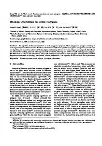
graph G I = PI n B, see Figure 5.1. This is performed by intersecting PI with each face g of A. In each column containing an edge of I, the processors intersect PI with its edge for g. These intersection points are then sorted on the line of intersection PI n g. Each processor containing an intersection point aquire the ID of the next processor containing the next intersection point in this sorted order. Using this information the intersection points are linked to form edges. Two consecutive intersection points are linked if the edge formed by them lies inside g which can be checked in constant time. These edges are the edges of the cross-sectional graph PI n B. However, the intersection points on partnered edges are duplicates of the same vertex and the generated edges on individual faces are not linked up. The pair of processors containing partnered edges remove this duplicacy with proper linking of edges across faces in constant time
P
f
FIG U RE 1: The Cross-sectional Graph G I
= PI n B
5
ALGORITHMIC DETAILS
6
since each one knows the ID of the other one. This completes the formation of G f for each fEB in parallel. Parallel computation of intersection points of Pf n 9 for each face pair
f, 9 takes constant
time. The sorting step takes 0 (log2 n) time. The rest of the linking process takes constant time per processor. Putting all these together, constructing the cycles of the cross-sectional graphs for all faces of B takes 0(1og2 n) time.
5.2
Clipping cross-sectional graphs
The cross-sectional graph G f and
f lie on the same plane and we are interested in constructing
the polygon G f n f. For this G f is clipped with the edges of f to construct G f n f. It may happen that some cycles of
f are not intersected by G f. We will discuss this case later. Below
we describe the method of computing the cycles in Gf n f arising out of the intersection of a single cycle of G f with a single cycle of f. Consider the subarray M containing the edges of
f. Note that
G f is constructed in all
columns of this subarray. All these copies of G f are used to construct G f
n f.
A processor
containing an edge e of f and an edge e' of G f computes the intersection ene'. We sort all such intersections and the end points of e along the columns of M. We also sort the intersection points and the end points of e' along e'. For this we sort these intersection points and the end points of e' along the row of M containing e'. Each intersection point i is involved in a cross formed by two edges e E
f and e'
E G f. Among four wedges formed by this cross, only one
belongs to G f n f. Consider the edge e" E {e, e'} that is directed away from i on this wedge. If e" = e(e') then an edge of G f n f is formed between i and the next intersection point sorted
along the column (row). In effect, this creates the edges of Gf n
f which are spread over the
block. Again, other than sorting, all operations take constant time giving an
o (1og2 n)
time to
construct G f n f for all fEB.
5.3
Detecting Redundant Cycles
Some of the cycles of G f and
f are not intersected by any edge. Let W be this set of cycles.
These cycles become part of Gf n
f by the above computations though some of them should
5
ALGORITHMIC DETAILS
7
not be, see Figure 5.3. We discard the redundant cycles as follows. A cycle of
f
that is in W is either lying completely inside A (inside cycles) or outside A
(outside cycles). The outside cycles should be deleted. No edge of these outside cycles intersect A. A ray in the direction of the edge intersects A at even number of points if it is on an outside
cycle as opposed to inside cycles. We compute this information for each edge of Let the processors in column j contain an edge of
f.
f
as follows.
Each of these processors p shoots a
ray r in the direction of the edge and computes its intersection with the face 9 of A whose edge is kept in p. All these intersection points are lexicographically sorted with their coordinates. Since an intersection point is computed more than once, multiple copies of a particular point appear consequtively in this sorted sequence. To detect the number of such distinct intersection points, a processor that has an intersection point different from the next processor in this sorted sequence gets a value 1. All other processors get a value O. We count the number of faces of A intersected by the ray r by counting the number of processors containing 1. This count is
obtained by computing the cumulative sum of the weights of the processors in the column j in a leader processor
e.
This takes O(log n) time. The processor
odd or even. If it is even then
e checks if the cumulative sum is
en A is empty and e broadcasts this information to all processors
in its column. Thus, at the expense of O(log2 n) parallel steps, all processors having an edge e
FIGURE 2: Nested Cycles of a Cross-sectional Graph
5
ALGORITHMIC DETAILS
8
of B knows if e n A is empty. After computing cycles in W, the processors remove those edges (hence cycles) that are designated to be outside A. This eliminates the redundant cycles of
f. Any edge of the
redundant cycles in G f appears only in one cycle. On the other hand, an edge of An B appears in two cycles. The redundant edges of G f are detected later when partnered edges of A n Bare associated. The edges that are not associated with any partnered edge are eliminated.
5.4
Arranging the Output
After the above computations, each cycle on a face
f E
An B is represented by a sequence
of processors that contain a directed edge on the cycle and a pointer to the next processor containing the next directed edge on the cycle. We also maintain an index in each of these processors identifying the face to which the corresponding cycle belong. The edges of the faces of A n B are stored over the entire array. First of all, we need to collect the edges of these faces and arrange them in an orderly manner so that the output conforms to the input. Secondly, we need to detect the partnered edges. The processors containing the edge of a cycle c of a face select a leader £ among them. This can be done in
o (log n)
step. The size s of c can be detected in another O(log n) step.
The leader £ forms the tuple (i, s) where i is the index of
f. All such leaders are then sorted
lexicographically on the basis of these tuples. Let £1, £2, ..., £m be this sorted sequence with the sizes
SI, S2, ... , Sm'
For each processor
£k
cumulative sum
Sk
= 2:7=1 Sj is computed.
be done in O(log2 n) steps. The processors that have the leader Sk, Sk
+ 1, ... around
the cycle starting at
processor with the assigned value
S
£k.
£k
are assigned the numbers
This step also can be done in
broadcasts the edge of
This can
o (log2 n) steps.
A
f to all processors in the column s.
This arranges all the edges of A n B in such a way that all edges of a cycle are put in adjacent columns and all cycles of a face are put in adjacent blocks. To detect the partnered edges, each processor form a tuple with the coordinates of the end points of the edges. These tuples are sorted lexicographically. Two partnered edges have same tuples and thus they come next to each other in this sorted order. Thus each of the two processors containing partnered edges aquire the pointers for the other from this sorted
6
CONCLUSION
9
sequence in constant time. This completes the arrangement of the output.
6
Conclusion
We have described an efficient algorithm for Boolean Set operations between two arbitrary manifold polyhedra, on a MIMD distributed memory machine. For two polyhedra with O(n) edges each, our algorithms run in O( log2n ) time on an n 2 processor MIMD machine. We are currently implementing our scheme on our resident 64 processor nCUBE2 hypercube MIMD machine. The nCUBE2 has a Sparcstation server as a front-end from which both data and programs are downloaded to the individual processors. The downloading being a serial process is relatively time consuming compared to the actual parallel computation time. Our Boolean operation algorithm outputs polyhedra in the same distributed data structure as the input. This allows the cascading of multiple Boolean set operations, (as well as execution of other modeling operations) on the parallel machine before serializing the final result on the front-end computer. To this effect, we are currently exploring parallel finite element mesh generation algorithms on our distributed polyhedra data structure.
References [1] Aggarwal, A., Chazelle, B., Guibas, L., O'Dunlaing, C., and Yap, C., (1988), "Parallel Computational Geometry," Algorithmica, 3,3, 293-327. [2] Akl, S., (1985) Parallel Sorting Algorithms, Academic Press. [3J Atallah, M.J. and Goodrich, M.T. (1985), "Efficient Parallel Solutions to Geometric Problems," Proc. 1985 Int'l Conf. on Parallel Processing, 411-417. [4] Batcher, K. E., (1968) "Sorting Networks and their Applications", Proc. of the 1968 AFIPS Spring Joint Computer Conference, vol 32.
[5] Karasick, M., (1988) "On the Representation and Manipulation of Rigid Solids", Ph.D. Thesis, Computer Science, McGill University, Montreal, Canada.
REFERENCES
10
[6] Laidlaw, D., Trumbore, W., and Hughes, J., (1986) "Constructive Solid Geoemtry for Solid Objects", Proc. of the ACM Siggraph Conference, 20, 161-170. [7] Mantyla, M., (1980) "Boolean Operations of2-Manifolds Trhough Vertex Neiborhood Classification", ACM Transactions on Graphics, 5, 1 - 29. [8] nCUBE Corporation, (1991) nCUBE 2 Programmer's Guide. [9] Requicha, A., and Voelcker, H., (1985) "Boolean Operations in Solid Modeling: Boundary Evaluation and Merging Algorithms", Proc. of IEEE, vol 73, 30 - 44. [10] Thibault, W., and Naylor, B., (1987) "Set Operations on Polyhedra using Binary Space Partitioning Trees", Proc. of the ACM Siggraph Conference, 21, 153 - 162