Checking Temporal Properties of Discrete, Timed and Continuous Behaviors Dedicated to B.A. Trakhtenbrot on his 85th Birthday
Oded Maler1 , Dejan Nickovic1 and Amir Pnueli2,3 1
3
Verimag, 2 Av. de Vignate, 38610 Gi`eres, France [Dejan.Nickovic | Oded.Maler]@imag.fr 2 Weizmann Institute of Science, Rehovot 76100, Israel New York University, 251 Mercer St. New York, NY 10012, USA
[email protected]
Words, even infinite words, have their limits. Abstract. We survey some of the problems associated with checking whether a given behavior (a sequence, a Boolean signal or a continuous signal) satisfies a property specified in an appropriate temporal logic and describe two such monitoring algorithms for the real-time logic MITL.
1 Introduction This paper is concerned with the following problem. Given a temporal property ϕ how to check that a given behavior ξ satisfies it. Within this paper we assume that the behavior to be checked is produced by a model of a dynamical system S, although some of the techniques are applicable to behaviors generated by real physical systems. Unlike formal verification which aims at showing that all behaviors generated by S satisfy ϕ, here S is used to generate one behavior at a time and can thus be viewed as a black box. This setting has been studied extensively in recent years both in the context of digital hardware, under the names of “dynamic” verification, or assertion checking as well as for software, where it is referred to as runtime verification [HR02a,SV03]. We will use the term monitoring. In this framework the question of coverage, that is, finding a finite number of test cases whose behavior will guarantee overall correctness, is delegated outside the scope of the property monitor. This approach can be used when the system model is too large to be verified formally. It is also applicable when the “model” in question is nothing but a hardly-formalizable simulation program, as is often the case in electrical simulation of circuits. On the other hand, the explicit presentation of ξ itself, rather than using the generating model S, raises new problems. Most of the work described in this paper has been performed within the European project PROSYD4 with the purpose of extending some ingredients of verification methodology from digital (discrete) to analog (continuous and hybrid) systems. Consequently, we treat systems and behaviors described at three different levels of abstraction 4
IST-2003-507219 PROSYD (Property-Based System Design).
(discrete, timed and continuous). Hence we find it useful to start with a generic model of a dynamical system defined over an abstract state space which evolves in an abstract time domain, see also [M98,M02]. The three models used in the paper are obtained as special instances of this model. States and Behaviors A model S of a system is defined over a set V = {x1 , . . . xn } of state variables, each ranging over a domain Xi . The state space of the system is thus X = X1 × · · · × Xn . The system evolves over a time domain T which is a linearlyordered set. A behavior of the system is a function from the time domain to the state space, ξ : T → X. We consider complete behaviors, where ξ is defined all over T , as well as partial behaviors where ξ is defined only on a downward-closed subset of T , that is, some interval of the form [0, r). We use the notation ξ[t1 , t2 ] for the restriction of ξ to the interval [t1 , t2 ] and let ξ[t] = ⊥ when t ≥ r. We denote the set of all possible (complete and partial) behaviors over a set X by X ∗ .5 Systems The dynamics of a system S is defined via a rule of the form x0 = f (x, u) which determines the future state x0 as a function of the current state x and current input u ∈ U . As mentioned earlier, we do not have access to f and our interaction with the model is restricted to stimulating it with an input ν ∈ U ∗ and then observing and checking the generated behavior ξ ∈ X ∗ . Properties Regardless of the formalism used to express it, a property ϕ defines a subset Lϕ of X ∗ . A property monitor is a device or algorithm for deciding whether a given behavior ξ satisfies ϕ (denoted by ξ |= ϕ) or, equivalently, whether ξ ∈ Lϕ . The paper starts with properties of discrete (digital) systems, a well-studied and mature domain, where some of the problems associated with monitoring (non-causality of the specification formalism, satisfiability by finite traces, online vs. offline) are already manifested. We then move to timed discrete systems, whose behaviors can be viewed as continuous-time Boolean signals, which raise a lot of new issues such as sampling, event detection, variability bounds, etc. Most of the paper will investigate monitoring at this level of abstraction where we made some original contributions. Finally we move to continuous (analog) signals which, in addition to dense time, admit also numerical real values. Although for many types of properties (and in particular those expressible in our signal temporal logic [NM07,MN04]) checking continuous properties can be reduced to checking timed properties, there are further issues, such as approximation errors, raised by the continuous domain and by the manner in which signals are generated by numerical simulators.
2 Discrete (Digital) Systems: Properties Discrete models are used for modeling digital hardware (at gate level and above) as well as software. At this level of abstraction the set N of natural numbers is taken as 5
For discrete time behaviors, it is common to use X ∗ for finite behaviors and X ω for infinite ones, but these distinctions are less meaningful when we come to continuous behaviors.
the underlying time domain. In this case the difference between ξ[t] and ξ[t + 1] reflects the changes in state variables that took place in the system within one clock cycle (hardware) or one program step (software).6 The state space of digital systems is often viewed as the set Bn of Boolean n-bit vectors.7 Behaviors are, hence, n-dimensional Boolean sequences generated by system models which are essentially finite automata (transition systems) which can be encoded in a variety of formalisms such as systems of Boolean equations with primed variables or unit delays, hardware description languages at various levels of abstraction, programming languages, etc. Semantically speaking, a property is a subset of the set of all sequences (also known in computer science as a formal language) indicating the behaviors that we allow the system to have. Such subsets can be defined syntactically using a variety of formalisms such as logical formulae, regular expressions or automata that accept them. In this paper we focus on temporal logic [MP92,MP95] which can be viewed as a useful syntactic sugar for the first-order fragment of the monadic logic of order [T61]. This section does not present new results but is rather a synthetic survey of the state-of-the-art which can serve as an entry point to the vast literature and which, we feel, is a pre-requisite for understanding the timed and continuous extensions. 2.1
Temporal Logic (Future)
The temporal logic of linear time (LTL) is perhaps the most popular property specification formalism. In a nutshell it is a language for specifying certain relationships between values of the state variables at different time instants, that is, at different positions in the sequence. For example, we may require that whenever x1 = 1 at position t then x2 = 0 at position t+3. A property monitor is thus a device that observes sequences and checks whether they satisfy all such relationships. We repeat briefly some standard definitions concerning the syntax and semantics of LTL. By semantics we mean the rules according to which a sequence is declared as satisfying or violating a formula ϕ. The syntax of LTL is given by the following grammar: ϕ := p | ¬ϕ | ϕ1 ∨ ϕ2 | ° ϕ | ϕ1 Uϕ2 , where p belongs to a set P = {p1 , . . . , pn } of propositions indicating values of the corresponding state variable. The basic temporal operators are next (°), which specifies what should hold in the next step and until (U), which requires ϕ1 to hold until ϕ2 becomes true, without bounding the temporal distance to this becoming. From these basic LTL operators one can derive other standard Boolean operators as well as temporal operators such as eventually (♦) and always (¤): ♦ϕ = 6
7
T
Uϕ
and
¤ϕ = ¬♦¬ϕ.
We mention here the existence and usefulness of asynchronous (event triggered rather than time triggered) systems and models, where the interpretation of a step is different. In software, as well as in high-level models of hardware, systems may include state variables ranging over larger domains such as bounded and unbounded numerical variables or dynamically-varying data structures such as queues and trees, but, at least in the hardware context, those can be encoded by bit vectors.
Models of LTL are Boolean sequences of the form ξ : N → Bn . We also use p to denote the sequence obtained by projecting a sequence ξ on the dimension corresponding to p. The satisfaction relation (ξ, t) |= ϕ, indicating that sequence ξ satisfies ϕ starting from position t, is defined inductively as follows: (ξ, t) |= p (ξ, t) |= ¬ϕ (ξ, t) |= ϕ1 ∨ ϕ2 (ξ, t) |= °ϕ (ξ, t) |= ϕ1 Uϕ2
↔ p[t] = 1 ↔ (ξ, t) 6|= ϕ ↔ (ξ, t) |= ϕ1 or (ξ, t) |= ϕ2 ↔ (ξ, t + 1) |= ϕ ↔ ∃t0 ≥ t (ξ, t0 ) |= ϕ2 and ∀t00 ∈ [t, t0 ), (ξ, t00 ) |= ϕ1
(ξ, t) |= ♦ϕ (ξ, t) |= ¤ϕ
↔ ∃t0 ≥ t (ξ, t0 ) |= ϕ ↔ ∀t0 ≥ t (ξ, t0 ) |= ϕ
A sequence ξ satisfies ϕ, denoted by ξ |= ϕ, iff (ξ, 0) |= ϕ. 2.2
Temporal Logic (Past)
The past fragment of LTL is defined by a syntax similar to the future fragment where the next and until operators are replaced by previously (° - ) and since (S). As with future LTL, useful derived operators are sometime in the past ♦ - and always in the past ¤- defined as ♦ - ϕ = T Sϕ and ¤- ϕ = ¬♦ - ¬ϕ Their semantics is given by (ξ, t) |= ° -ϕ ↔ t = 0 or (ξ, t − 1) |= ϕ (ξ, t) |= ϕ1 Sϕ2 ↔ ∃t0 ∈ [0, t] (ξ, t0 ) |= ϕ2 and ∀t00 ∈ (t0 , t], (ξ, t00 ) |= ϕ1 (ξ, t) |= ♦ -ϕ (ξ, t) |= ¤- ϕ
↔ ∃t0 ∈ [0, t](ξ, t0 ) |= ϕ ↔ ∀t0 ∈ [0, t] (ξ, t0 ) |= ϕ
A finite sequence satisfies a past property ϕ if it satisfies it from the last position “backwards”, that is, ξ |= ϕ if (ξ, |ξ|) |= ϕ.
3 Discrete Systems: Checking Temporal Properties We describe here the fundamental problems associated with checking temporal properties as well as the common approaches for tackling them. These are problems that exist already in the simplest model of Boolean sequences and are propagated, with additional complications to the timed and continuous domains. 3.1
Causality and Non-determinism
A major difficulty in checking properties expressed in future LTL is due to the noncausal definition of the satisfaction relation. To see what this means it might be helpful
to look at the definition of LTL semantics as a procedure which is recursive on both the structure of ϕ and on the sequential structure of ξ. This procedure is called initially with ϕ and with ξ[0] as arguments because we want to determine the satisfiability of ϕ from position zero. Then the semantic rules “call” the procedure recursively with sub formulae of ϕ and with further positions of ξ. In other words, the satisfiability of ϕ at time t may depend on the value of ξ at some future time instant t0 ≥ t. Even worse, some temporal operators refer to future time instants in a quantified manner, for example, requiring some p to hold in all future time instants. The satisfiability of such a property may sometime be determined only at infinity, that is, “after” we can be sure that no instance of ¬p is observed. Note that for past LTL, the recursion goes backward in time and the satisfaction of a past formula ϕ by a sequence ξ at position t is determined according to the values of ξ at the interval [0, t] and in this sense, past LTL is causal. However it has been argued that the futuristic specification style is more natural for humans. The past fragment of LTL admits an immediate translation to deterministic automata and a simple monitoring procedure [HR02b] based on this observation. The “classical” theoretical scheme for using LTL in formal verification is based on translating a formula ϕ into a non-deterministic automaton over infinite sequences (an ω-automaton) Aϕ that accepts exactly the sequences that satisfy it. The non determinism is needed to compensate for the non causality: the automaton has to “guess” at time t whether future observations at some t0 > t will render ϕ satisfied at t, and split the computation into two paths according to these predictions. A path that made a wrong prediction will be aborted later, either within a finite number of steps (if the guess is falsified by some observation) or via the ω-acceptance condition (if the falsification is due to non-occurrence of an event at infinity). Satisfiability of the formula can thus be determined by checking whether the ω-language accepted by Aϕ is not empty. This reduces to checking the existence of an accepting cycle in Aϕ which is reachable from an initial state. Verification is achieved by checking whether S may generate an infinite behavior rejected by Aϕ (or accepted by A¬ϕ ). It should be noted that simplified procedures have been developed and implemented when the property in question belongs to a subclass of LTL, such as safety. 3.2
Evaluating Incomplete Behaviors
In monitoring we do not exploit the model S that generates the sequences, but rather observe sequences as they come. The major problem here, with respect to the standard semantics of LTL which is defined over complete infinite sequences, is the impossibility to observe infinite sequences in finite time.8 Hence, the extension of LTL semantics to incomplete behaviors is a major issue in monitoring. After having observed a finite sequence ξ we can be in one of the following three basic situations with respect to a property ϕ: 8
To be more precise, there are some classes of infinite sequences such as the ultimately-periodic ones, that admit a finite representation and an easily-checkable satisfiability, however we work under the assumption that we do not have much control over the type of sequences provided by the simulator and hence we have to treat arbitrary finite sequences. It is worth noting that if S is input-deterministic then an ultimately-periodic input induces an ultimately-periodic behavior.
1. All possible infinite completions of ξ satisfy ϕ. Such a situation may happen, for example, when ϕ is ♦p and p occurs in ξ. In this case we say that ξ positively determines ϕ. 2. All possible infinite completions of ξ violate ϕ. For example when ϕ is ¤¬p and p occurs in ξ. In this case we say that ξ negatively determines ϕ. 3. Some possible completions of ξ do satisfy ϕ and some others violate it. For example, any sequence where p has not occurred has extensions that satisfy, as well as extensions that violate, formulae such as ♦p or ¤¬p. In this case we say that ξ is undecided. It should be noted that the “undecided” category can be refined according to both methodological, quantitative, and logical considerations. One might want to distinguish, for example, between “not yet violated” (in the case of ¤¬p) and “not yet satisfied” (in the case of ♦p). The quantitative aspects enter the picture as well because the longer we observe a sequence ξ free of p, the more we tend to believe in the satisfaction of ¤¬p, although the doubt will always remain. On the other hand, the satisfaction of a formula like °k p, a shorthand for °(°(. . . ° p) . . .)), although undecided for sequences shorter than k, will be revealed in finite time. The most general type of answer concerning the satisfiability of ϕ by a finite sequence ξ would be to give exactly the set of completions of ξ that will make it satisfy ϕ, defined as ξ\ϕ = {ξ 0 : ξ · ξ 0 |= ϕ}. Positive and negative determination correspond, respectively, to the special cases where ξ\ϕ = X ∗ and ξ\ϕ = ∅. This “residual” language can be computed syntactically as the left quotient (“derivative”) of ϕ by ξ. In certain situations we would like to give a decisive answer at the end of the sequence. In the case of positive and negative determination we can reply with a yes/no answer. More general rules for assigning semantics to every finite sequence have been proposed [LPZ85,EFH+ 03]. Let us consider some sub-classes of LTL formulae for which such a finitary semantics clearly makes sense. The simplest among those is bounded-LTL where the only temporal operator is next and where satisfiability of a formula ϕ at time 0 is always determined by the values of the sequence up to some t ≤ k, with k being a constant depending on ϕ. Note that this class is not as useless as it might seem: one can use “syntactic sugar” operators such as ¤[0,r] ϕ as shorthand for Vr−1 i i=0 (° ϕ). The implication for monitoring is that every sufficiently-long sequence is determined with respect to such formulae (see also [KV01]). The next class is the class of safety properties9 where the only quantification of the time variable is universal as in ¤ϕ. It is not hard to see that ω-languages corresponding to such formulae consist of infinite words that do not have a prefix in some finitary language. While monitoring a finite sequence ξ relative to such a formula, we can be in either of the following two situations. Either such a prefix has been observed and hence any continuation of ξ will be rejected and ξ can be declared as violating, or no 9
To be more precise safety properties can be written as positive Boolean combinations of formulae of the form ¤ϕ where ϕ is a past property, and eventuality properties are negations of safety properties.
such prefix has been observed but nothing prevents its occurrence in the future and ξ is undecided. A similar and dual situation holds for eventually property such as ♦ϕ that quantify existentially over time, and where an occurrence of a finitary prefix satisfying ϕ renders the sequence accepted. With respect to these sub-classes one can adopt the following policy: interpret any quantification Qt, Q ∈ {∀, ∃} as Qt ≤ |ξ| and hence a safety that has not been violated during the lifetime of ξ is considered as satisfied, and an eventuality not fulfilled by that time is interpreted as violated. This principle may be extended to more complex formulae that involve nesting of temporal operators but in this case the interpretation seems less intuitive. Let us remark that although models of past LTL are finite sequences, the problem of undecided sequences still exists. Consider for example the property ¤- p. As soon as ¬p is observed, we can say the the formula is negatively determined and need not wait for the rest of the sequence. On the other hand, as long as ¬p has not been observed, although the prefix satisfies the property we cannot give conclusive results until the “official” end of the sequence, because ¬p may always be observed in the next instant. Hence the treatment of past properties is not much different from future ones, except for the simpler construction of the corresponding automaton Naturally many solutions have been proposed to this problem in the context of monitoring and runtime verification and we mention few. The work of [ABG+ 00] concerning the FoCs property checker of IBM, as well as those of [KLS+ 02] are restricted to safety (prefix-closed) or eventuality properties and report violation when it occurs. On the other hand, the approach of giving the residual language is proposed in [KPA03] and [TR04] in the context of timed properties. A systematic study of the possible adaptation of LTL semantics to finite sequences (“truncated paths”) is presented in [EFH+ 03]. This semantics has been adopted by the semiconductor industry standard property specification language PSL [EF06]. Our approach to monitoring is invariant under all these semantical choices. As a minimal requirement for being used, the chosen semantics should associate with every formula ϕ a function Ωϕ : X ∗ → D which maps all finite sequences into a domain D that contains B (satisfied/violated) and is augmented with some additional values for undecided formulae. 3.3
Offline and Online Monitoring
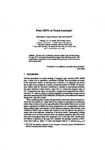
In this section we discuss different forms of interaction between the mechanism that generates behaviors and the mechanism that checks whether they satisfy a given property. The behaviors are generated by some kind of a simulator that computes states sequentially. Without loss of generality we may assume that the systems we are interested in are not reverse-deterministic and, hence, the natural way to generate behaviors is from the past to the future. One may think of three basic modes of interaction (see Figure 1): 1. Offline: The behaviors are completely generated by the simulator before the checking procedure starts. The behaviors are kept in a file which can be read by the monitor in either direction.
2. Passive Online: The simulator and the checker run in parallel, with the latter observing the behaviors progressively. 3. Active Online: There is a feed-back loop between the generator and the monitor so that the latter may influence the choice of inputs and, hence, the subsequent values of ξ. Such “adaptive” test generation may steer the system toward early detection of satisfaction or violation, and is outside the scope of this paper. Each behavior is a finite sequence ξ, whose satisfiability value with respect to ϕ is defined via Ωϕ (ξ) regardless of the checking method. However there are some practical reasons to prefer one method over the other. First, to save time, we would like the checking procedure to reach the most refined conclusions as soon as possible. In the offline setting this will only reduce checking time, while in the online setting the effects of early detection of satisfaction/violation can be much more significant. This is because in certain systems (analog circuits is a notorious example) simulation time is very long and if the monitor can abort a simulation once its satisfiability is decided, one can save a lot of time. The difference between online and offline is, of course, much more significant in situations where monitoring is done with respect to a physical device, not its simulated model. We discuss briefly several instances of this situation. The first is when chips are tested after fabrication by injecting real signals to their ports and observing the outcome. Here, the response time of the tester is very important and early (online) detection of violation can have economic importance. In other circumstances we may be monitoring a system which is already up and running. One may think of the supervision of a complex safety-critical plant where the monitoring software should alert the operator about dangerous developments that manifest themselves by property violation or by progress toward such violations. Such a situation calls for online monitoring, although offline monitoring can be used for “post mortem” analysis, for example, analyzing the “black box” after an airplane crash. Monitoring can be used for diagnosis and improvement of non-critical systems as well. For example analyzing whether the behavior of an organization satisfies some specifications concerning the business rules of the enterprise, e.g. “every request if treated within a week”. Such an application of monitoring can be done offline by inspecting transaction logs in the enterprise data base. In the sequel we describe three basic methods for checking satisfaction of LTL formulae by sequences. The Automaton-Based Method This is an online-oriented approach that follows the principles used in formal verification. To monitor a property ϕ we first construct the automaton Aϕ that accepts exactly the sequences satisfying ϕ and then let it read every sequence ξ as it is generated. There is a vast literature concerning the construction of automata from LTL formulae [VW86] and monitoring does not depend too much on the choice of the translation algorithm. We have, however a preference for the compositional construction, presented in [KP05] and extended for timed systems in [MNP06]. For each sub-formula ψ of ϕ, this procedure constructs a sequence χψ (ξ) indicating the satisfaction of ψ over time, that is χψ (ξ) has value 1 at t iff (ξ, t) |= ψ. There are two major problems that need to be tackled while employing this method. The first problem is that the natural automaton for ϕ will be an automaton over infi-
Input Generator
Simulator
File
Input Generator
Simulator
Monitor/checker
Input Generator
Simulator
Monitor/checker
Monitor/checker
Fig. 1. Offline, passive online and active online modes of interaction between a test generator and a checker.
nite sequences. This automaton needs to be transformed, via a suitable definition of acceptance conditions, into an automaton over finite sequences that realizes the chosen finitary semantics, as discussed in the previous section. For example, if our satisfiability domain consists of yes, no and undecided, we will output yes as soon as the automaton enters a state from which all the remaining paths are accepting (a positive “sink”) and no when we enter a negative sink. From all other states the output will be undecided. The second problem is that Aϕ is typically non-deterministic. It can be resolved in either of the following ways: 1) Feed the non-deterministic automaton with ξ while keeping track of all the states in which it can be at every time instant. This amounts to performing the classical “subset construction” on-the-fly; 2) Determinize the automaton offline, either using Safra’s algorithm for ω-automata [S88] or using a simpler algorithm adapted to the finitary semantics.
Purely-Offline Marking This is the first method we have developed to timed and continuous properties and will be described in more detail in Section 6.1. The procedure consists in computing χψ (ξ) for every sub-formula ψ of ϕ from the bottom up. It starts with the truth values of propositional formulae χp (ξ) given by the sequence ξ itself. Then, recursively, for each sub-formula ψ with immediate sub-formulae ψ1 and ψ2 such that χψ1 (ξ) and χψ2 (ξ) have already been computed, we compute χψ (ξ) following the semantic rules of LTL. The backward nature of these rules implies that the values of ξψ1 and ξψ2 at time t will “propagate” to values of ξψ at some t0 ≤ t. The satisfaction function χϕ for the main formula is computed at the end.
Incremental Marking This approach combines the simplicity of the offline procedure with the advantages of online monitoring in terms of early detection of violation or satisfaction. After observing a prefix of the sequence ξ[0, t1 ] we apply the offline procedure. If, as a result, χϕ (ξ) is determined at time zero we are done. Otherwise we observe a new segment ξ[t1 , t2 ] and then apply the same procedure based on ξ[0, t2 ]. A more efficient implementation of this procedure need not start the computation from scratch each time a new segment is observed. It will be often the case that χψ (ξ) for some sub-formulae ψ is already determined for some subset of [0, t1 ] based on ξ[0, t1 ]. In this case we only need to propagate upwards the new information obtained from ξ[t1 , t2 ], combined, possibly, with some additional residual information from the previous segment that was not sufficient for determination in the previous iterations. This procedure will be described in more algorithmic detail in Section 6.2. The choice of the granularity (length of segments) in which this procedure is invoked depends on trade-offs between the computational cost and the importance of early detection.
4 The Timed Level of Abstraction Coming to export the specification, testing and verification framework from the digital to the analog world, one faces two major conceptual and technical problems [M06]. 1. The state variables range over subsets of the set of real numbers that represent physical magnitudes such as voltage or current; 2. The systems evolve over a physical time scale modeled by the real numbers and not over a logical time scale defined by a central clock or by events. Mathematically speaking, the behaviors that should be specified and checked are signals, function from R≥0 to Rn rather than sequences from N to Bn or to some other finite domain. The first problem for monitoring is the problem of how to represent a signal defined over the real time axis inside the computer, given that it is a function defined over an infinite (and non-countable) domain. The very same problem is encountered, of course, by numerical simulators that produce such signals. Based on our conviction that the dense time problem is more profound than the infinite-state problem we use the following approach. Using a finite number of predicates over the continuous state space, analog signals are transformed into Boolean ones and are checked against properties expressed in a real-time temporal logic whose atomic propositions correspond to those predicates. This allows us to tackle the problem of dense time in isolation. Aspects specific to the continuous state space are discussed in Section 7. Note that one can naturally combine these predicates with genuine Boolean propositions to specify properties of hybrid systems (mixed-signal systems in the circuit jargon). Handling an infinite state space, such as the continuum, using finite formulae is a fundamental mathematical problem. In finite domains one can characterize every individual state by a distinct formula. For example, there is a bijection between Bn and the set of Boolean terms over {p1 , . . . , pn } which has one literal for each pi . The common
way to speak of subsets of infinite sets such as Rn is via predicates, functions from Rn to B, for example inequalities of the form xi < d. We thus adopt the following approach. Let µ1 , . . . , µm be m predicates of the form µ : Rn → B. These predicates define a mapping M : Rn → Bm assigning to every real point a Boolean vector indicating the predicates it satisfies. Applying this mapping in a pointwise fashion to an analog signal ξ : R≥0 → Rn we obtain a Boolean signal M (ξ) = ξ 0 : R≥0 → Bm describing the evolution over time of the truth values of these predicates with respect to ξ (see Figure 2). Events such as rising and falling in the Boolean signal correspond to some qualitative changes in the analog signal, for example threshold crossing of some continuous variable. This is an intermediate level of abstraction where we can observe the temporal distance between such events and need to confront the problems introduced by the dense time domain. Timed formalisms such as real-time temporal logics or timed automata are tailored for modeling, specification, verification and monitoring at this level of abstraction, which in addition to its applicability to analog circuits, is also very useful to model phenomena such as delays in digital circuits and execution times of software and, in fact, anything in life that can be modeled as a process where some time has to elapse between its initiation and termination.10 Input
and
Delayed
Signals
1
0.8
0.6
0.4
0.2
0
s = x1 ||x2
−0.2
−0.4
−0.6
−0.8
−1
0
50
100
150
200
250
300
2 Time
offset:
0
p1 = x1 > 0.7
1 0 −1
2 1
p2 = x2 > 0.7
0 −1
2 1 0 −1
Fig. 2. A 2-dimensional continuous signal and the 2-dimensional Boolean signal obtained from it via the predicates x1 > 0.7 and x2 > 0.7. 2 1 0 −1
2 1 0 −1
4.1
0
50
100
150
200
250
300
Dense-Time Signals: Representation Time offset: 0
The major problems in handling Boolean signals by computerized tools are due to the properties of the time domain. In digital systems we have the discrete order (N, 0) and an ideal mathematical signal ξ that satisfies the property but which passes very close to zero at some points. We can easily transform ξ into a signal ξ 0 which is very close to ξ under any reasonable continuous metric, but according to the metric induced by the property, these signals are as distant as can be: one of them satisfies the property and the other violates it (see Figure 8). Moreover, if the sojourn time of a signal below zero is short, an arbitrary shift in the sampling can make the monitor miss the zero-crossing event and declare the signal as satisfying (see Figure 9). In this sense properties are not robust as small variations in the signal may lead to large variations in its property satisfaction. Let us mention some interesting ideas due to P. Caspi [KC06] concerning new metrics for bridging the gap between the continuous and the discrete points of view. Such metrics are expressible, by the way, in STL [NM07]. The abovementioned issues can be handled pragmatically in our context, without waiting for a completely-satisfactory theoretical solution to this fundamental prob15
16
It is worth noting that some models used for rapid simulation of transistor networks cannot always be viewed as continuous dynamical systems in the classical mathematical sense. For systems which are stable the quality can be improved indefinitely.
ξ0
ξ
t
t
µ(ξ 0 )
µ(ξ) t
t
Fig. 8. Two signals which are close from a continuous point of view, one satisfying the property ¤(x > 0) and one violating it.
t
Fig. 9. Shifting the sampling points, zero crossing can be missed.
t
lem. The following assumptions facilitate the monitoring of sampled continuous signals against STL properties, passing through the timed abstraction: 1. Sufficiently-dense sampling: the simulator detects every change in the truth value of any of the predicates appearing in the formula at a sufficient accuracy. This way the positive intervals of all the Boolean signals that correspond to these predicates are determined. This requirement imposes some level of sophistication on the simulator that has to perform several back-and-forth iterations to locate the time instances where a threshold crossing occurs. Many simulation tools used in industry have already such event-detection features. A survey of the treatment of discontinuous phenomena by numerical simulators can be found in [Mos99]. 2. Bounded variability: some restrictive assumptions can be made about the values of the signal between two sampling points t1 and t2 . For example one may assume that ξ is monotone so that if ξ[t1 ] ≤ ξ[t2 ] then ξ[t01 ] ≤ ξ[t02 ] for every t01 and t02 such that t1 < t01 < t02 < t2 . An alternative condition could be a condition a-la Lipschitz: |ξ[t2 ] − ξ[t1 ]| ≤ K|t2 − t1 |. Such conditions guarantee that the signal does not get wild between the sampling points, otherwise property checking based on these values is useless. Under such assumptions every continuous signal which is given by a discrete-time representation, based on sufficiently-dense sampling, induces a well-defined Boolean signal ready for MITL monitoring. Let us add at this point a general remark that the standards of exactness and exhaustiveness as maintained in discrete verification cannot and should not be exported to the continuous domain, and even if we are not guaranteed that all events are detected, we can compensate for that by using safety margins in the predicates and properties.
8 Monitoring STL Properties In this section we illustrate the monitoring of STL properties against signals produced by the numerical simulator Matlab/Simulink, used mainly for control and signal-processing applications, but also for modeling analog circuits at the functional level of abstraction. The waveforms presented here are the output of our first prototype of analog monitoring tool, which parses STL properties and applies the offline marking procedure described in Section 6.1. 8.1
Following a Reference Signal
As a first example consider the property ϕ1 : ¤[0,300] ((x1 > 0.7) ⇒ ♦[3,5] (x2 > 0.7)) which requires that whenever x1 crosses the threshold 0.7, so does x2 within t ∈ [3, 5] time units. We fix x1 to be the sinusoid x1 [t] = sin(ωt),
d1
d2
Fig. 10. Sufficiently-dense sampling with respect to the two thresholds d1 and d2 . The set of sampling points consists of a uniform grid augmented with the threshold-crossing points.
and let x2 be a signal generated by x2 [t] = sin(ω(t + d)) + θ where d is a random delay ranging in [3, 5] degrees and θ is an additive random noise. The marking procedure is illustrated in Figure 11. The Boolean signals corresponding to the atomic propositions p1 and p2 are derived from the sampled analog signal. From there the truth values of the sub-formulae ♦[3,5] (x2 > 0.7), (x1 > 0.7) ⇒ ♦[3,5] (x2 > 0.7) are marked as intermediate steps toward the marking of ϕ1 which is satisfied in this example. In Figure 12 we apply the same procedure to check ϕ1 against a signal in which x2 was generated with a much larger additive noise θ ∈ [−0.5, 0.5]. The fluctuations in the value of x2 are reflected in the Boolean abstraction p2 and lead to a violation of the property at some points where x1 > 0.7 is not followed by x2 > 0.7 within the pre-specified delay. 8.2
Stabilizability
The second example is a very typical stabilizability property used extensively in control and signal processing. The system in question is supposed to maintain a controlled variable y around a fixed level despite disturbances x coming from the outside world. The actual system used to generate this example is a water-level controller for a nuclear plant. The disturbances come from changes in the system load that trigger changes in the operations of the reactor which, in turn, influences the water level, see [Don03]. Other instances of the same type of problem may occur when the voltage of a cirucit
Input
and
Delayed
Signals
1
0.8
0.6
0.4
0.2
0
s = x1 ||x2
−0.2
−0.4
−0.6
−0.8
−1
0
50
100
150
200
250
300
150
200
250
300
2 Time
offset:
0
p1 = x1 > 0.7
1 0 −1
2 1
p2 = x2 > 0.7
0 −1
2 1
♦[3,5] p2
0 −1
2
p1 → ♦[3,5] p2
1 0 −1
2
¤[0,300] (p1 → ♦[3,5] p2 )
1 0 −1
0
50
100
Time offset: 0
Fig. 11. A 2-dimensional signal satisfying the property ¤[0,300] ((x1 > 0.7) ⇒ ♦[3,5] (x2 > 0.7)). Boolean signals correspond to the evolution of the truth values of sub-formulae over time.
Input
and
Delayed
Signals
1
0.8
0.6
0.4
0.2
0
s = x1 ||x2
−0.2
−0.4
−0.6
−0.8
−1
0
50
100
150
200
250
300
150
200
250
300
2 Time
offset:
0
p1 = x1 > 0.7
1 0 −1
2 1
p2 = x2 > 0.7
0 −1
2 1
♦[3,5] p2
0 −1
2
p1 → ♦[3,5] p2
1 0 −1
2
¤[0,300] (p1 → ♦[3,5] p2 )
1 0 −1
0
50
100
Time offset: 0
Fig. 12. A 2-dimensional signal violating the property ¤[0,300] ((x1 > 0.7) ⇒ ♦[3,5] (x2 > 0.7)).
has to be kept constant despite variations in the current due to changes in the circuit workload. We want y to stay always in the interval [−30, 30] (except, possibly, for an initialization period of duration 300) and if, due to a disturbance, it goes outside the interval [−0.5, 0.5], it should return to it within 150 time units and stay there for at least 20 time units. The whole property is ϕ2 : ¤[300,2500] ((|y| ≤ 30) ∧ ((|y| > 0.5) ⇒ ♦[0,150] ¤[0,20] (|y| ≤ 0.5))). The results of applying our offline monitoring procedure to this formula appear in Figures 13 and 14. When the disturbance is well-behaving, the property is verified, while when the disturbance changes too fast, the property is violated both by overshooting below −30 and by taking more than 150 time units to return to [−0.5, 0.5].
9 Conclusions Motivated by the exportation of some ingredients of formal verification technology toward analog circuits and continuous systems in general, we embarked on the development of a monitoring procedure for temporal properties of continuous signals. During the process we have gained better understanding of temporal satisfiability in general as well as of the relation between real-time temporal logics and timed automata. The ideas presented in this paper have been implemented into an analog monitoring tool AMT [NM07] that has been applied to real-life case studies.
References [ABG+ 00] Y. Abarbanel, I. Beer, L. Glushovsky, S. Keidar, and Y. Wolfsthal, FoCs: Automatic Generation of Simulation Checkers from Formal Specifications, CAV’00, 538-542, LNCS 1855, Springer, 2000. [AD94] R. Alur and D.L. Dill, A Theory of Timed Automata, Theoretical Computer Science 126, 183-235, 1994. [AFH96] R. Alur, T. Feder, and T.A. Henzinger, The Benefits of Relaxing Punctuality, Journal of the ACM 43, 116-146, 1996. [AH92] R. Alur and T.A. Henzinger, Logics and Models of Real-Time: A Survey, REX Workshop, Real-time: Theory in Practice, 74-106. LNCS 600, Springer, 1992. [A04] E. Asarin, Challenges in Timed Languages, Bulletin of EATCS 83, 2004. [ACM02] E. Asarin, P. Caspi and O. Maler, Timed Regular Expressions, The Journal of the ACM 49, 172-206, 2002. [BBDE+ 02] I. Beer, S. Ben David, C. Eisner, D. Fisman, A. Gringauze, and Y. Rodeh, The Temporal Logic Sugar, CAV’01, LNCS 2102, Springer, 2002. [BBKT04] S. Bensalem, M. Bozga, M. Krichen, and S. Tripakis, Testing Conformance of Realtime Applications with Automatic Generation of Observers, RV’04, 2004. [Don03] A. Donz´e. Etude d’un Mod`ele de Contrˆoleur Hybride. Master’s thesis, INPG, 2003. [EF06] C. Eisner and D. Fisman, A Practical Introduction to PSL, Springer, 2006. [EFH+ 03] C. Eisner, D. Fisman, J. Havlicek, Y. Lustig, A. McIsaac, and D. Van Campenhout, Reasoning with Temporal Logic on Truncated Paths, CAV’03, 27-39, LNCS 2725, Springer, 2003.
Disturbance Signal
100 50 Analog Response y(t)
50 0 −50 −100 p = y ∈ (−0.5, 0.5)
2 1 0 −1 q = y ∈ (−30, 30)
2 1 0 −1
¤[0,20] p
2 1 0 −1
♦[0,150] ¤[0,20] p
2 1 0 −1
¬p → ♦[0,150] ¤[0,20] p
2 1 0 −1
¬p → ♦[0,150] ¤[0,20] p
2 1 0 −1
¤[300,2500] (q ∧ (¬p → ♦[0,150] ¤[0,20] p))
2 1 0 −1
0
500
1000
1500
2000
2500
3000
Fig. 13. A disturbance signal and an analog response y satisfying the stabilizability property ¤[300,2500] ((|y| ≤ 30) ∧ ((|y| > 0.5) ⇒ ♦[0,150] ¤[0,20] (|y| ≤ 0.5))).
Disturbance Signal
100 50 Analog Response y(t)
50 0 −50 −100 p = y ∈ (−0.5, 0.5)
2 1 0 −1 q = y ∈ (−30, 30)
2 1 0 −1
¤[0,20] p
2 1 0 −1
♦[0,150] ¤[0,20] p
2 1 0 −1
¬p → ♦[0,150] ¤[0,20] p
2 1 0 −1
¬p → ♦[0,150] ¤[0,20] p
2 1 0 −1
¤[300,2500] (q ∧ (¬p → ♦[0,150] ¤[0,20] p))
2 1 0 −1
0
500
1000
1500
2000
2500
3000
Fig. 14. A disturbance signal and an analog response y violating the stabilizability property ¤[300,2500] ((|y| ≤ 30) ∧ ((|y| > 0.5) ⇒ ♦[0,150] ¤[0,20] (|y| ≤ 0.5))).
[GD00]
M.C.W. Geilen and D.R. Dams, An On-the-fly Tableau Construction for a Real-time Temporal Logic, FTRTFT’00, 276-290. LNCS 1926, Springer, 2000. [Gei02] M.C.W. Geilen, Formal Techniques for Verification of Complex Real-time Systems, PhD thesis, Eindhoven University of Technology, 2002. [Gei03] M.C.W. Geilen, An Improved On-the-fly Tableau Construction for a Real-time Temporal Logic, CAV’03, 394-406, LNCS 2725, Springer, 2003. [HR02a] K. Havelund and G. Rosu (editors), Runtime Verification RV’02, ENTCS 70(4), 2002. [HR02b] K. Havelund and G. Rosu, Synthesizing Monitors for Safety Properties, TACAS’02, 342-356, LNCS 2280, Springer, 2002. [Hen98] T.A. Henzinger, It’s about Time: Real-time Logics Reviewed, CONCUR’98, 439454, LNCS 1466, Springer, 1998. [HR04] Y. Hirshfeld and A. Rabinovich Logics for Real Time: Decidability and Complexity, Fundamenta Informaticae 62, 1-28, 2004. [KP05] Y. Kesten and A. Pnueli, A Compositional Approach to CTL∗ Verification, Theoretical Computer Science 331, 397-428, 2005. [KC06] C. Kossentini and P. Caspi, Approximation, Sampling and Voting in Hybrid Computing Systems, HSCC, to appear, 2006. [Koy90] R. Koymans, Specifying Real-time Properties with with Metric Temporal Logic, Real-time Systems, 255-299, 1990. [KLS+ 02] M. Kim, I. Lee, U. Sammapun, J. Shin, and O. Sokolsky, Monitoring, Checking, and Steering of Real-time Systems, RV’02, ENTCS 70(4), 2002. [KPA03] K.J. Kristoffersen, C. Pedersen, and H.R. Andersen, Runtime Verification of Timed LTL using Disjunctive Normalized Equation Systems, RV’03, ENTCS 89(2), 2003. [KT04] M. Krichen and S. Tripakis, Black-box Conformance Testing for Real-time Systems, SPIN’04, 109-126, LNCS 2989, 2004. [KV01] O. Kupferman and M.Y. Vardi, On Bounded Specifications, LPAR’01, 24-38, LNCS 2250, 2001. [Mos99] P.J. Mosterman, An Overview of Hybrid Simulation Phenomena and their Support by Simulation Packages, HSCC’99, 165-177, LNCS 1569, 1999. [LPZ85] O. Lichtenstein, A. Pnueli and L.D. Zuck, The Glory of the Past, Conf. on Logic of Programs, 196-218, LNCS, 1985. [M98] O. Maler, A Unified Approach for Studying Discrete and Continuous Dynamical Systems, CDC, 2083-2088, IEEE, 1998. [M02] O. Maler, Control from Computer Science, Annual Reviews in Control 26, 175-187, 2002. [M06] O. Maler, Analog Circuit Verification: a State of an Art ENTCS 153, 3-7, 2006. [MN04] O. Maler and D. Nickovic, Monitoring Temporal Properties of Continuous Signals, FORMATS/FTRTFT’04, 152-166, LNCS 3253, 2004. [MNP05] O. Maler, D. Nickovic and A. Pnueli, Real Time Temporal Logic: Past, Present, Future, FORMATS’05, 2-16, LNCS 3829, 2005. [MNP06] O. Maler, D. Nickovic and A. Pnueli, From MITL to Timed Automata, FORMATS’06, 274-289, 2006. [MNP07] O. Maler, D. Nickovic and A. Pnueli, On Synthesizing Controllers from BoundedResponse Properties, CAV’07, 95-107, 2007. [MP92] Z. Manna and A. Pnueli, The Temporal Logic of Reactive and Concurrent Systems Specification, Springer, 1992. [MP95] Z. Manna and A. Pnueli, Temporal Verification of Reactive Systems: Safety, Springer, 1995. [NM07] D. Nickovic and O. Maler, AMT: A Property-Based Monitoring Tool for Analog Systems, FORMATS’07, 304-319, 2007.
[S88] [SV03] [T61] [TR04] [Tri02] [VW86]
S. Safra, On the Complexity of ω-Automata, FOCS’88, 319-327, 1988. O. Sokolsky and M. Viswanathan, editors. Runtime Verification RV’03. ENTCS 89(2), 2003. B.A. Trakhtenbrot, Finite Automata and the Logic of One-place Predicates, DAN SSSR 140, 1961. P. Thati and G. Rosu, Monitoring Algorithms for Metric Temporal Logic Specifications, of RV’04, 2004. S. Tripakis, Fault Diagnosis for Timed Automata, FTRTFT’02, 205-224, LNCS 2469, Springer, 2002. M.Y. Vardi and P. Wolper, An Automata-theoretic Approach to Automatic Program Verification, LICS’86, 322-331, IEEE, 1986.