In our proposed scheme, a pixel is marked as an edge pixel, if there ..... R. Wildes, et. al., âVideo georegistration: algorithm and quantitative evaluation,â Proc.
Detection and Localization of Edge Contours Dongjiang Xu and Takis Kasparis School of Electrical Engineering and Computer Science, University of Central Florida Orlando, FL 32816
ABSTRACT Edge contour extraction plays an important role in computer vision because edge contours are relatively invariant to the changes of illumination conditions, sensor characteristics, etc. In particular, edge contours can be used as matching primitives for correspondence determination, an important step in video geo-registration. In this paper, we present a new approach for edge contour extraction based on a three-step procedure that using a RCBS-based scheme, inherently more accurate results can be produced, even though the edge model used for edges is relatively simple. We also present recursive filters that can efficiently smooth splines by approximating a signal with a complete set of coefficients subject to certain regularization constraints. We demonstrate our method on both synthetic and real images. Keywords: Edge contours, zero crossings, B-spline, LoG
1. INTRODUCTION Edge detection is a fundamental operation in low-level computer vision with a plethora of techniques and several distinct paradigms1 that have been proposed. Despite these efforts, the solutions to the edge contour extraction problem are still unsatisfactory for some application, where the subsequent processing stages depend primarily on the performance of the edge detector. In an image, an edge refers to an occurrence of rapid image intensity transition7. An edge detector is to locate these transitions, and its resulting edge map identifies the location of them, together with some gradient and direction information. In order to use such an edge map in higher-level processes such as stereo and motion analysis, the next step is to identify those edge points that should be grouped together into edge segments2. However, real image data are often very diverse, and edges occur over a wide range of scales. As a result, the edge maps are cluttered with discontinued edge segments with degraded accuracy of location and isolated edge points. This type of edge map carries unexpected errors into the later stages of image processing tasks. Edge maps provide a concise and accurate representation of the boundaries of objects and regions in an image. The geometric information contained in these stable edge contours is often sufficient to spatially match two images so that corresponding pixels in the two images correspond to the same physical region of the scene being imaged3. Actually, the goal of image matching is to establish the correspondence between two images and determine the geometric transformation that aligns one image with the other. The major advantage of contour-based approach over a correlationbased, is its insensitivity to scaling, rotation, and intensity changes as well as its low computational low cost. Video georegistration, a process of associating 3D world coordinates with videos, is different from image registration, since most approaches of the latter employ only simple image-to-image mappings, which can’t correctly model the projections between the 3D world and 2D frames9. However, after projecting the reference and video imagery to a common coordinate frame, the subsequent matching between them can be largely 2D in nature, and a reliable and robust correspondence determination is essential to successfully register video images to a reference image8, 9. At present, major video geo-registration schemes still choose normalized cross-correlation as a matching measure for correspondence determination, which is a computationally intensive process. In this paper, our objective is to develop a framework for accurately detecting and localizing edge contours in aerial images, which can be used as matching primitives, instead of the correlation-based matching measures. In the next section we briefly review the previous work on edge contour detection and localization. The proposed scheme is
Geo-Spatial and Temporal Image and Data Exploitation III, Nickolas L. Faust, William E. Roper, Editors, Proceedings of SPIE Vol. 5097 (2003) © 2003 SPIE · 0277-786X/03/$15.00
79
explained in Section 3. Experiment results are demonstrated in Section 4. We conclude with some discussions in Section 5.
2. PREVIOUS WORK Torre and Poggio10 have suggested that edge detection is a problem in numerical differentiation and showed that numerical differentiation of images is an ill-posed problem in the sense of Hadamard. Differentiation amplifies high frequency components. In practical situations, image data are contaminated by noise and differentiation will enhance high frequencies of the noise. However, differentiation is a mildly ill-posed problem10, which can be transformed into a well-posed problem by several methods. Marr and Hildreth11 proposed convolving the signal with a rotationally symmetric Laplacian of Gaussian (LoG) mask and locate zero-crossings of the resulting output, where the amount of smoothing is controlled by the variance of the Gaussian. There is a good theoretical foundation for using such a method because the Gaussian is an optimal filter for edge detection due to its localization properties in both the spatial and frequency domains. Additionally, Gaussian smoothing is also computationally inexpensive. However, the fundamental conflict encountered in edge detection is to eliminate noise without distorting its localization, namely noise immunity and accurate localization. The Gaussian filters, while smoothing the noise, also remove genuine high-frequency edge features to be sought, degrade edge localization and the detection of low-contrast edges. Edges can be weak but well localized. Such edges, also representing a major fraction of information content in an image like the strong edges, maybe severely blurred by effective noise-reduction with circularly symmetric operators. The LoG operator has been applied to extract edge contours4, 5. As explained above, the main objection to the use of this operator has been that it has poor localization properties. The proposed scheme5 also chooses good control points on the non-closed edge contours, where uncertain errors will be introduced. To overcome these problems, many authors have proposed multi-scale techniques12 in order to reach the conflicting goals of detecting the existence of intensity discontinuities and of determining their exact location. The whole edge detection scheme requires that irrelevant details and noise being suppressed. Multiple scale algorithms can improve detection of weak edges and those that are close together. But, there are two major problems with multi-scale techniques, namely how to select the step between operator’s scales for 2D images and effectively combine the edge contours from different scales. Williams and Shah3 present a theoretical analysis of the movement of idealized edges, two adjacent step edges with the same or opposite polarity. However, it is very difficult to find a robust scale space combining approach in 2D case since edges obtained from the 2D filtered signals behave in a much more complex way in scale space than those from 1D filtered signals. In addition, combination of edge contours itself is an image matching problem, and computationally expensive. Although Canny edge detector has better SNR and edge location accuracy than that of LoG-based approach, the local extrema of its output may have unconstrained behaviors13,24 in the scale space. Moreover, the 2D Canny detector, where is obtained by simply extending the 1D result based on the constant cross-section 2D edge model, is not optimal in 2D cases.
3. THE EDGE CONTOUR EXTRATION SCHEME The surface fitting method is an effective method used to detect edges based on the assumption that a 2D image is a discrete array of intensity values obtained from sampling a real-valued function f defined on the domain of the image 6, 14
. To this end, some parametric form of the underlying function f is assumed and the discrete sampled intensity values in the finite size of neighborhood are used to estimate those parameters. Edge decisions are made based on the estimated underlying function f .
Because such an edge detection scheme involves a process of fitting the basis functions to the sampled image data, the chosen basis function set must be complete in the sense of approximating all the edge features being sought in a scene. Otherwise, some edges, not in the feature space spanned by the selected basis function set, can’t be detected.
Our proposed method applies regularized cubic B-spline fitting5 (RCBS) for edge detection based on a one-dimension surface model from Nalwa-Binford16, where 2D image data can be reduced into 1D by projecting the data in the
80
Proc. of SPIE Vol. 5097
direction of least local intensity changes. It is effective because the original image data can be smoothed to reduce noise while preserving discontinuities. The primary advantage of this one-dimension surface model is that it explicitly exploits the directional characteristics of edges, which differs from Haralick’s 2D surface fitting approach14. Figure 1 shows the block diagram of the basic structure of the proposed edge contour extraction scheme. First, gradient and orientation at each pixel are estimated. Subsequently, RCBS fitting is applied for edge detection. In the end, edge contours of aerial images are generated after post-processing of edge maps from edge detection. Our proposed scheme generates better results than LoG-based methods, and the detected contours, open or closed, can directly be used for the matching stage.
Gradient and Orientation Estim ation
Aerial Images
Edge D etection using RCB S Fitting
P ost-P rocessing: Edge C ontours
Figure 1: The block diagram of the edge contour extraction scheme
3.1. Gradient and Orientation Estimation Directionality in edge detection is not a new concept. First, a number of templates that could match an ideal edge model at various orientations are applied, and then edges and their directions are detected from results of the largest search and the thresholding of the outputs. Some simple and popular examples are Roberts’ operator, Prewitt operator, and Sobel operator. On the use of these operators, however, there seems to have been considerable confusion between gradients and edges17, where the magnitude of the gradient is used to locate the positions of edges. Actually, there is no such a direct correspondence between them. If we take noise and edge imperfection into consideration, weak but well localized edges are difficult to be detected using such simple thresholding schemes, since edges are not at the locations of high gradient, but at locations of spatial gradient maxima. In our proposed scheme, a pixel is marked as an edge pixel, if there is a zero crossing of second derivative of the underlying function f taken in the direction of the estimated gradient. Although there is a correspondence between the continuous and the discrete image, this is not the case between the continuous gradient and the discrete gradient due to inherent errors involved in gradient operators. Shigeru17 presents optimal gradient operators using a newly derived consistency criterion, which is based on an orthogonal decomposition of the difference between a continuous gradient and discrete gradients into the intrinsic smoothing effect and the selfinconsistency involved in the operator. To obtain accurate gradient information, the author suggests that reduction of the self-inconsistency is of the primary importance, where the exact shape of the smoothing filter can be determined secondarily. The power spectrum of the consistent gradient image is expressed as: 2
Gx (u, v ) + G y (u , v ) = 2
2 1 2 uH ( u , v ) + vH ( u , v ) F (u , v ) . i j 2 2 u +v
(1)
The power spectrum of the inconsistent gradient image is express as: 2 2 ~ ~ Gx (u , v ) + G y (u , v ) =
2 1 2 uH j (u, v) − vH i (u , v ) F (u , v ) . 2 u +v 2
(2)
Therefore, optimal gradient operators can be obtained by minimizing the inconsistent power
Proc. of SPIE Vol. 5097
81
J≡
1 2
1 2
~ G x (u , v ) ∫ ∫ 1 1 − − 2
2
2 ~ + G y (u, v ) dudv =
1 2
1 2
∫ ∫ Ψ (u, v ) P (u, v ) dudv
→ min
(3)
− 12 − 12
2
where
Ψ (u , v) =
2 1 uH j (u , v ) − vH i (u, v ) . 2 u +v
(4)
2
2
P(u, v ) = E[ F (u, v ) ].
(5)
To obtain the best result, we choose Shigeru’s optimum 5x5 gradient operators, and compare them with Prewitt operators with a size of 3x3 and Zuniga-Haralick’s integrated directional derivative gradient operator (IDDG) with a size of 5x5. Figure 2 presents the results of the above three operators on a synthetic checkerboard image with added Gaussian noise. Fig. 2a shows the synthetic checkerboard image with noise having σ=50. Fig. 2b presents edges produced by RCBS based on Shigeru’s 5x5 gradient operators, Fig. 2c presents edges produced by RCBS based on IDDG operators, and Fig. 2d is the result of RCBS based on Prewitt operators. It can be seen that, when the noise level is high, the Prewitt operator produces the noisiest results because of errors in estimating gradient orientation. This is expected since operators with small support are always more sensitive to noise. Fig. 2c displays the results from IDDG operators, which are less noisy than that of the Prewitt operators, however, more true edges are missed, which could be from bigger errors in estimating the edge orientation. To this end, we took a slice near the position of a potential edge in the original image and tested with two levels of Gaussian noise (σ=20, 50), and plotted the estimated gradient orientations from these three operators along the slice in Figures 2e and 2f respectively. We notice that orientation errors from IDDG operators are at some points worse than those of Prewitt operators, and these errors generate more missed detections at true edge pixels. Therefore, using a bivariate cubic polynomial to model the image would also be noise sensitive when the noise level is high. As is evident in these figures, RCBS based on Shigeru’s gradient operators gives the best result (Fig. 2a) regarding to both noise immunity and the accuracy of localization.
(a)
82
Proc. of SPIE Vol. 5097
(b)
(c)
(d)
(e)
(f)
Figure 2: Comparison on synthetic images using different gradient operators. (a) Checkerboard image with size 300x300 (noise σ=50). (b) Shigeru’s operator. (c) Haralick’s operator. (d) Prewitt’s operator. (e) Comparison between three operators (noise σ= 20). (f) Comparison between three operators (noise σ= 50).
3.2. Edge Detection by Regularized Cubic B-Spline Fitting Splines are piecewise polynomials with pieces that are smoothly connected together. B-splines are splines which have smallest possible support, in other words, they are zero on a large set. The essential property of B-splines of order n is to provide a basis of the subspace of all continuous piecewise polynomial functions of degree n with derivatives up to n-1 that are continuous everywhere on the real line18. In the case of equally spaced integral knot points, any unction φ (x) of this space can be represented as: n
φ n ( x) =
∑ c (i ) β ( x − i ) +∞
n
(6)
i = −∞
where
β n (x) denotes the normalized B-spline of order n. Because the function φ n (x) is uniquely determined by its B-
spline coefficients {c(i)} , the crucial step in B-spline interpolation is to determine the coefficients of this expansion such that
φ n (x) matches the values of some discrete sequence {g (k )} at the knot points: φ n (k ) = g (k ) for
{k = −∞,...,+∞} . Proc. of SPIE Vol. 5097
83
Figure 3 (a) cubic B-spline. (b) The mask used by RCBS, and its orientation is determined by Shigeru’s operators.
In Figure 3(a) we show the following closed form representation of the cubic B-spline:
2 / 3 − x 2 + x 3 / 2, 0 ≤ x < 1 β 3 ( x) = (2 − x )3 / 6, 1≤ x < 2 0, 2≤ x
(7)
Chen and Yang5 proposed a RCBS-based edge detection scheme, which uses a set of cubic B-splines to approximate the underlying 3D intensity surface along the gradient direction in Fig 3(b). Because real image data are corrupted by noise, a regularization term is introduced to suppress its effect. Reinsh19 and Schoenberg20 have proposed the use of smoothing spline. Given a set of discrete signal values {g ( k )} , the smoothing spline21,23 gˆ ( x) of order 3 is defined as the function that minimizes: d
ε = ∑ [g ( xk ) − gˆ ( xk )] + λ ∫ 2
2 s
k
gˆ ( x ) =
∑ c (i ) β ( x − i )
M +1
2
2
gˆ ( x ) 2 2 dx = ε A + λε r 2 dx
3
(8)
(9)
i=0
where λ is a given positive parameter. The choice of λ depends on which of these two conflicting goals is accorded the greater importance. A set of cubic B-splines basis function β ( x) is used for the fitting between the interval [1, M], 3
where M is the number of the grid pixels to be fitted. The minimization of
ε s2 can be achieved by setting the partial
derivatives of ε s with respect to {c(i )}, k = 0,..., M + 1 to zero. This leads to the solution of a system of M+1 linear equations, and can be solved by matrix operations. 2
In the following, we show how to efficiently determine the coefficients of the smoothing spline by digital filtering21 instead of conventional matrix operations. Applying the properties of the B-splines, a simpler form of
ε r2 =
84
Proc. of SPIE Vol. 5097
∑ (d
k ∈Z
( 2)
) (
)
∗ c (k ) d ( 2) ∗ b13 ∗ c (k )
ε r2 is therefore: (10)
Then,
ε s2 can be expressed in terms of discrete convolutions
ε s2 =
∑ (g (k ) − (b ∗ c(k ))) + λ ∑ (d 3 1
k ∈Z
2
k ∈Z
( 2)
) (
)
∗ c (k ) d ( 2 ) ∗ b13 ∗ c (k )
(11)
which, using the inner product notation, is also equivalent to:
ε s2 =< g , g > −2 < g , b13 ∗ c > + < b13 ∗ c, b13 ∗ c > + λ < d ( 2) ∗ c, d ( 2) ∗ c ∗ b13 >
(12)
The smoothing spline coefficients are found by setting to zero the derivative of this expression with respect to c(k ) . By using the properties of the inner product calculus21, we find that
(b13 )' ∗ g (k ) = (b13 )' ∗ b13 ∗ c(k ) + λ (d ( 2)' ∗ d ( 2) ∗ (b13 )' ∗ c(k ))
(13)
Applying z transform on both sides, we have
B13 ( z −1 )G ( z ) = B13 ( z −1 ) B13 ( z )C ( z ) + λD ( 2) ( z ) D ( 2) ( z −1 ) B13 ( z −1 )Y ( z )
(14)
By solving for C (z ) , we have
1 G ( z ) = Sλ3G ( z ) −1 2 B ( z) + λ ( z − 2 + z ) 1 B13 ( z ) = (z + 4 + z −1 ) 6 C ( z) =
(15)
3 1
(16)
This above expression clearly shows that the coefficients of the smoothing spline can be determined by digital filtering, 3
as illustrated in Figure 4. The transfer function of the smoothing spline filter S λ ( z ) corresponds to a IIR filter, which can be most efficiently implemented recursively. After we determine the cubic B-spline coefficients, we can directly obtain a general cubic B-spline differentiator (first-, second-, and third-order derivatives) shown in Figure 4. B-spline Coefficients 1st order derivative
1 − z −1
2 1
C ( z)
2nd order derivative
g (k ) 3
Sλ ( z )
direct transform
z − 2 + z −1
1 1
B (z)
3rd order derivative
z − 3 + 3 z −1 − z −2
C10 ( z )
n
Figure 4 Block diagram of a B-spline differentiator using the smoothing spline ( C1
( z ) , B1n ( z ) : B-spline kernels)
Proc. of SPIE Vol. 5097
85
We mark the center pixel of the operator support as an edge pixel if for some r , r < r0 , where r0 is smaller than half ' '' ''' the length of the side of a pixel, gˆ α ( r ) = 0 , gˆ α ( r ) ≠ 0 , and gˆ α ( r ) is greater than its neighbors’, namely a non-
maximum suppression step22. For every marked edge point, the edge strength is defined as the slope at each zero''
crossing of gˆ α (r ) in the estimated gradient direction. 3.3 Edge Contours: Post-processing of RCBS Edge Maps The results from RCBS edge maps maybe “noisy”, but the edges are continuous and thin. The noisy edge points can be discarded easily in the post-processing stage using the edge strength defined above. First, a hysteresis thresholding22 is applied to the edge map. This algorithm is basically the same as the one used in the Canny algorithm. The low threshold is set to preserve the whole contour around the region boundary without incurring discontinuities at weak edge points. The high threshold is chosen large enough to avoid spurious edges. This two-threshold scheme is implemented by scanning the 2D edge strength array. Contour search is initiated wherever one point with a value greater than the high threshold is scanned. The same search operation continues until the whole edge strength array has been scanned. The contours are then divided into two categories, closed contours and open contours. Second, different thinning rules are applied. For example, if the point is adjoining a diagonal edge, then remove it. These rules are applied to each identified edge pixel in the edge map sequentially left to right and top to bottom, which can be achieved using only one pass of the algorithm.
4. EXPERIMENT RESULTS Because of space limitations, only results from one aerial image are presented. Fig 3 shows the results of the LoG-based and RCBS-based schemes with different scales. Fig. 5a is the original real image and Fig. 5b is the output of the LoGbased scheme (σ=1). Fig. 5c is the output of the LoG-based scheme (σ=3), Fig. 5d the output of RCBS-based scheme (λ=0.0000001) at a fine scale, and Fig. 5e the output of RCBS-based scheme (λ=0.01) at a medium scale.
(a)
86
Proc. of SPIE Vol. 5097
(b)
(c)
(d)
(e) Figure 5: Examples of edge contour extraction by (a) original aerial image, (b) edge contours from LoG (σ=1), (c) edge contours from LoG (σ=3), (d) edge contours from RCBS (λ=1.0E-7), (e) edge contours from RCBS (λ=1.0E-1)
Note that the size of LoG operators is different at different scale and the size is bigger at coarse scales. On the other hand, in the RCBS-based scheme the operator’s support is fixed. Our experiments use a rectangular window of size 5x7. For LoG operators, the detection of edges with accurate position depends on the scales we choose26. When we choose a smaller scale (σ=1), the resulted edge contours by LoG operators are shown in Fig 5b. Obviously, the edges are very noisy and include a lot of false edges. In order to suppress the effect of noise, we try a bigger scale having σ=3 and the result is shown in Fig. 5c. As it is expected, the noise is greatly suppressed, but we have further degraded the localization of edge contours. In addition, note also the large influence of each edge on one another at a coarse scale for the LoG operator because of its corresponding bigger operator size26. Fig. 5d and 5e show the results from our proposed RCBSbased scheme. Obviously, it produces much better results compared with those of the LoG-based scheme. We test it using two different scales ((λ=1.0E-7 and 1.0E-1). From the figures we can see that it can effectively suppress the noise, even at the fine scale (λ=1.0E-7). At medium scale (λ=1.0E-1), the localization of edge contours only shift very slightly. In conclusion, our proposed RCBS-based scheme is an effective way to control the balance between the two conflicting performance requirements for real images, namely noise immunity and accurate localization.
Proc. of SPIE Vol. 5097
87
5. SUMMARY AND CONCLUSIONS We have presented a new approach for edge contour extraction based on a three-step procedure. In the first step we obtain greatly improved estimated gradient information from Shigeru’s operators. The second step applies RCBS edge detection, which is an effective way to control the balance between the two conflicting performance requirements, namely noise immunity and accurate localization. The third step post-processes the resulted edge map using some strategies, which generate qualified edge contours for higher visual processing tasks. The experiment results indicate that our proposed scheme has better performance in both noise immunity and localization than that of LoG-based schemes. For some applications with time constraints, digital filtering techniques have been applied for solving the problem of regularized cubic B-spline fitting instead of the matrix approaches25. There is much work yet to be done. The balance of the operator’s support size and the regularization parameter with the noise immunity and the localization requirements should be further researched. Most existing algorithms in the literature treat edge detection a purely local process, which can’t guarantee the connections between the detected edge points. As a result, the output edge map often contains many broken segments. Accordingly, future research work should focus on taking a global view towards edge detection using its related properties, such as position, curvature, orientation, and contrast, in order to suppress the effect of noise and generate more manageable 2D edge contours for the stage of matching process.
REFERENCES 1.
2. 3. 4. 5. 6. 7. 8. 9. 10. 11. 12. 13. 14. 15. 16. 17.
88
M.D. Heath, S. Sarkar, T. Sanocki, and K.W. Bowyer, “A robust visual method for assessing the relative performance of edge-detection algorithms,” IEEE Trans. Pattern Anal. Machine Intell., Vol. 19, pp. 1338-1359, 1997. D.J. Williams and M. Shah, “Edge contours using multiple scales,” CVGIP, Vol. 51, pp. 256-274, 1990. X. Dai and S. Khorram, “A feature-based image registration algorithm using improved chain-code representation combined with invariant moments,” IEEE Trans. Geosci. Remote Sensing, Vol. 37, pp. 2351-2362, 1999. H. Li, B. S. Manjunath, and S. K. Miltra, “A contour-based approach to multisensor image registration,” IEEE Trans. Image Processing, Vol. 4, No. 3, 1995. G. Chen and Y. H. Yang, “Edge detection by regularized cubic B-spline fitting,” IEEE Trans. Systems, Man, and Cybernetics, Vol. 25, pp. 636-643, 1995. R. M. Haralick and L. Watson, “A facet model for image data,” Computer Graphics and Image Processing, Vol. 15, pp. 113-129, 1981. J. Koplowitz and V. Greco, “On the edge localization error for local maximum and zero-crossing edge detectors,” IEEE Trans. Pattern Anal. Machine Intell., Vol. 16, pp. 1207-1212, 1994 R. Wildes, et. al., “Video georegistration: algorithm and quantitative evaluation,” Proc. IEEE International Conference on Computer Vision, pp. 343-350, 2001 R.W. Cannata, et. al., “Autonomous video registration using model parameter adjustments,” Proc. 29th Applied Imagery Pattern Recognition Workshop, pp. 215-222, 2000. V. Torre and T. Poggio, “On edge detection,” IEEE Trans. Pattern Anal. Machine Intell., Vol. PAMI-8, pp. 147163, 1986. D. Marr and E. Hildreth, “Theory of edge detection,” Proc. R. Soc. Lond., Vol. B 207, pp.187-217, 1980. F. Bergholm, “Edge focusing,” IEEE Trans. Pattern Anal. Machine Intell., Vol. PAMI-9, pp. 726-741, 1987. R.J. Qian and T.S. Huang, “Optimal Edge Detection,” IEEE Image Trans. Image Processing, Vol. 5, pp. 1215-1220, 1996. R.M. Haralick, “Digital step edges from zero crossing of second directional derivatives,” IEEE Trans. Pattern Anal. Machine Intell., Vol. PAMI-6, pp. 58-68, 1984. O. A. Zuniga and R.M. Haralick, “Integrated directional derivative gradient operator,” IEEE Trans. Systems, Man, and Cybernetics, Vol. SMC-17, pp. 508-517, 1987. V.S. Nalwa and T.O. Binford, “On Detecting Edges,” IEEE Trans. Pattern Anal. Machine Intell., Vol. PAMI-8, pp. 699-714, 1986. S. Ando, “Consistent Gradient Operators,” IEEE Trans. Pattern Anal. Machine Intell., Vol. 22, pp. 252-265, 2000.
Proc. of SPIE Vol. 5097
18. M. Unser, A. Aldroubi, and M. Eden, “Fast B-spline transforms for continuous image representation and interpolation,” IEEE Trans. Pattern Anal. Machine Intell., Vol. 13, pp. 277-285, 1991. 19. C.H. Reinsh, “Smoothing by spline functions,” Numer. Math., Vol. 10, pp. 177-183, 1967. 20. I.J. Schoenberg, “Spline functions and the problem of graduation,” Proc. Nat. Acad. Sci., Vol. 52, pp. 947-950, 1964. 21. M. Unser, A. Aldroubi, and M. Eden, “B-spline signal processing: part I − theory,” IEEE Trans. Signal Processing, Vol. 41, pp. 821-833, 1993. 22. J. Canny, “A computational approach to edge detection,” IEEE Trans. Pattern Anal. Machine Intell., Vol. PAMI-8, pp. 679-698, 1986. 23. M. Unser, A. Aldroubi, and M. Eden, “B-spline signal processing: part II − efficient design and applications,” IEEE Trans. Signal Processing, Vol. 41, pp. 834-848, 1993. 24. A. Yulle and T.A. Poggio, “Scaling theorems for zero crossings,” IEEE Trans. Pattern Anal. Machine Intell., Vol. PAMI-8, pp. 15-25, 1986. 25. K. Liang, T. Tjahjadi, and Y-H. Yang, “Bounded diffusion for multiscale edge detection using regularized cubic Bspline fitting,” IEEE Trans. Systems, Man, and Cybernetics—Part B: Cybernetics, Vol. 29, pp. 291-297, 1999. 26. A. Huertas and G. Medioni, “Detection of intensity changes with subpixel accuracy using Laplacian-Gaussian masks,” IEEE Trans. Pattern Anal. Machine Intell., Vol. PAMI-8, pp. 651-664, 1986.
Proc. of SPIE Vol. 5097
89