2180
IEEE TRANSACTIONS ON POWER SYSTEMS, VOL. 29, NO. 5, SEPTEMBER 2014
Development of Low-Voltage Load Models for the Residential Load Sector Adam J. Collin, Member, IEEE, George Tsagarakis, Student Member, IEEE, Aristides E. Kiprakis, Member, IEEE, and Stephen McLaughlin, Fellow, IEEE
Abstract—A bottom-up modeling approach is presented that uses a Markov chain Monte Carlo (MCMC) method to develop demand profiles. The demand profiles are combined with the electrical characteristics of the appliance to create detailed time-varying models of residential loads suitable for the analysis of smart grid applications and low-voltage (LV) demand-side management. The results obtained demonstrate significant temporal variations in the electrical characteristics of LV customers that are not captured by existing load profile or load model development approaches. The software developed within this work is made freely available for use by the community. Index Terms—Load modelling, low-voltage (LV) network, Markov processes, power demand, residential load sector.
I. INTRODUCTION
T
HE influence of load characteristics on the operation and performance of electrical power systems is widely recognized. Accordingly, significant effort has been expended in developing load models for a range of power system studies, e.g., [1]–[3]. However, since the last major review of load models in 1995 [1], there have been many changes in the operation of the electrical power system and in the characteristics of loads, resulting in a need to update existing load models and produce new ones. This is reflected by a renewed interest in both industry and academia [4]. One of the main areas where this is particularly evident is in the modelling of the residential customers connected to the low-voltage (LV) distribution network. Traditionally, these networks and loads would have been represented by bulk aggregate load models for the analysis of medium and high-voltage networks, e.g., [2], [5], [6], but there is a need for better representation of these networks, and the connected load, to support the growing number of research areas associated with the LV networks, e.g., demand-side management (DSM) and electric vehicle integration. Manuscript received June 12, 2013; revised September 23, 2013 and November 14, 2013; accepted December 20, 2013. Date of publication February 06, 2014; date of current version August 15, 2014. The work was supported by the Research Councils UK Energy Programme under Grant EP/I000496/1. Paper no. TPWRS-00765-2013. A. J. Collin, G. Tsagarakis, and A. E. Kiprakis are with the Institute for Energy Systems, School of Engineering, The University of Edinburgh, Edinburgh EH9 3JL, U.K. (e-mail:
[email protected];
[email protected]; Aristides.
[email protected]). S. McLaughlin is with the School of Engineering and Physical Sciences, Heriot-Watt University, Edinburgh EH14 4AS, U.K. (e-mail:
[email protected]). Digital Object Identifier 10.1109/TPWRS.2014.2301949
Recent research on the modelling of residential customers has focused on representing the influence of user behavior characteristics on energy use patterns, e.g., [7]–[11], and the physical components within the aggregate load, e.g., [12]–[15]. However, the correct representation of load in power system studies requires both of these components: the load profile, which specifies how the power demand of the modelled load varies across the specified time, and the electrical load model, which specifies how the electrical characteristics of the load, i.e., how the power is drawn from the supply system, change with respect to time. Although the development of residential customer load profiles and models of the individual load components are relatively well represented in existing literature, there is still a lack of publicly available load models which bring these together. In this paper, the two research streams are combined to present a methodology for developing LV load models of the residential load sector. As the user behavior drives the electrical power demand, the modelling philosophy starts from the behavior of individual users which are represented using a Markov chain Monte Carlo (MCMC) modelling approach. The user activity profiles are then converted into active and reactive power demand profiles and the corresponding load models by using a large database of load statistics and a library of detailed load models of the individual load components which have been developed in previous research [16]–[20]. The methodology is implemented using the U.K. residential load sector as an example, and the various stages of the modelling process are validated against available U.K. statistics. The main contribution of this paper is the development of LV load models which are able to retain the stochastic variations which characterize the residential load sector. The load models are able to provide the expected temporal variations in the load profile but also provide more detailed information on the short-term and long-term variations of the electrical characteristics of the load than currently available load models of the residential load sector. Although any available load model form of the individual load components may be incorporated in the methodology, widely used static load model forms are used in this paper to illustrate and compare the temporal changes in load characteristics for three distinguishing system-loading conditions: maximum, minimum, and year average demand. Including these variations will allow for a more accurate assessment of the performance of LV networks, which is also demonstrated in this paper. The load modeling methodology is described in Section II and is illustrated in Section III by the U.K. residential load sector example, although the approach is more widely applicable. The
This work is licensed under a Creative Commons Attribution 3.0 License. For more information, see http://creativecommons.org/licenses/by/3.0/
COLLIN et al.: DEVELOPMENT OF LOW-VOLTAGE LOAD MODELS FOR THE RESIDENTIAL LOAD SECTOR
2181
TABLE I USER ACTIVITY STATE DEFINITIONS
Fig. 1. Load model development work flow.
developed load models are used to highlight differences in active and reactive power flows in Section IV. The conclusions are discussed in Section V. The developed software is made freely available for use by the community at [21].
II. LOAD-MODEL DEVELOPMENT METHODOLOGY In the residential load sector, power demand is driven by user behavior. The advent of “smartly driven” appliances may alter the time of use of certain loads, but the habitual patterns of the user will still drive the main periods of activity within the dwelling. For that reason, the modelling philosophy in this paper starts from consideration of the user activities. The power demand is intrinsically connected to a large number of factors which are typically used when defining user groups for modeling purposes, including: the characteristics of the user [7], [9], the number of household (HH) occupants [8], [11], the building type [9], and the time of year [9]. In the research presented here, each household is defined by the number of occupants in the household, which is hereafter referred to as the household size, and the user type of each occupant. Each household occupant is labeled as “working” or “not working,” with children classified as “working” occupants. Therefore, there are possible occupant combinations for each household size, e.g., household size one can have zero or one working occupant. More detailed user groups may be formed in future, e.g., based on the age of occupants, if required to analyze specific network scenarios. The modeling approach developed in this paper is divided into three stages: 1) user activity modeling; 2) conversion of user activities to electrical appliance use; 3) aggregation of the electrical appliances to build household power demand profiles and load models. These stages are presented in Fig. 1, which displays the information flows in the modeling framework. The input variables are configured by user-defined parameters which determine the aggregate size, the aggregate composition, the day of the week, and the month of the year. The simulation time step for user activity modelling is 10 min, due to the available input data, and is reduced to 1 min during the conversion to power demand to more accurately capture the short-term variations in load use.
A. User Activity Input Data The most prominent publicly available data for user activity information is in Time Use Surveys (TUS). The U.K. TUS (available from [22]) was used as the main source of input data for modeling the user activities in this study. Similar studies are available for a large number of countries around the world (an exhaustive TUS bibliography is available in [23]), to which the method described in this paper can be applied. B. User Activity Modelling To simplify the analysis, 13 user activity states are defined. The activity states include the main user activities which may result in electrical appliance use and also acknowledges the building occupancy, which is vital for the modelling of lighting and heating loads. As electrical appliances may be shared within multiple occupancy households, this functionality is also included in the relevant activity states. Table I contains further information on the defined user activity states. Due to the high variability, probabilistic approaches are normally applied to model user behavior. For example: the work in [7] utilizes probabilistic functions, while a Markov chain (MC) approach is implemented in [10], and [8] combines the two approaches. A thorough review of user-behavior modeling research is available in [24]. A combined MCMC approach is used to synthesize the user activity profiles in this paper. The MC transition probabilities are calculated by checking all transitions from state between time and and the total number of transitions between state and state between time and . The transition probability calculation is given by (1) where is the transition probability from state to state (which can include ) between time and , is the number of transitions from state to state between and , is the total number of transitions from state between and , and is the total number of activity states. In total, there are 143 transition matrices each containing 13 13 elements (for each household size and user type), i.e., one matrix for each
2182
IEEE TRANSACTIONS ON POWER SYSTEMS, VOL. 29, NO. 5, SEPTEMBER 2014
TABLE II POLYNOMIAL LOAD MODEL COEFFICIENTS [16], [19]
Fig. 2. Device sharing implementation example for a two-person household with two working occupants.
time step transition. The user activity state at is used to define the probability distribution of initial conditions . For multiple occupancy households, there is a probability that certain appliances will be used by more than one occupant at any given time. To calculate the device sharing probability, empirical data from the U.K. TUS “with” variable is analyzed to develop a probabilistic function. This variable has the following states: alone, with another person (household member), and with another person (not household member). This is a suitable indicator for device sharing, as all electrical appliances which can be shared will utilize at least one of the user’s senses and are not expected to be used within the same room at the same time. Therefore, if two or more users have the same activity state and “with” variables at the same time step, it is assumed that the electrical appliance is shared. The device sharing probability is determined by comparing all household users activity state and “with” variables at every time step. The is calculated by the ratio of users having the same activity and “with” variable to the users who have only the same activity , shown as follows:
(2) represents the number of occurwhere counter rences of activity at time for household members of household size , is the number of occurrences of activity at time which have the same “with” variable, and is sharing probability of members of household size sharing activity at time . This functionality is included in the modelling approach by including an additional stage after the user activity time series’ have been synthesized. An algorithm identifies every time period when multiple users have the same activity and compares the against a randomly generated uniform number . This is illustrated in Fig. 2 for a two-person household. The activity state of the secondary user is set to 1 if the electrical
device is shared, thus maintaining the correct household occupancy characteristics:
(3) where is the predetermined sharing probability for activity at time and is the random number. C. Conversion to Electrical Power Demand In the next stage of the modelling process, the synthesized user activity times series’ are converted into electrical loads using a database containing device ownership, usage, operating power range and standby power statistics [20]. The database also includes representation of the different operating phases of appliances, e.g., change in power demand during washing machine operating cycle, which are maintained within the developed time-varying load models (with full details available in [20]). These data are supplemented with the typical displacement power factor value and the electrical load model, which are presented in Table II in the following section. The majority of the user activity states defined in Table I have a direct conversion to an electrical appliance . For such activities, only the device ownership and statistical distributions of operating power are required to convert the activity to electrical power demand. However, for the activities which may or may not require an electrical appliance, additional time of use statistics are required. The user activity state at time is combined with and probabilistic functions of use of electrical appliance associated with user activity to convert to a power demand profile for appliance (4) where is a random value for power of appliance (in watts), with a probability distribution as described in [20]. The device use duration is selected from typical appliance usage profiles and requires the simulation time step to be converted to 1 min. This allows for the correct representation of loads with use duration less than 10 min and is implemented by randomly allocating the device start time within the 10-min period. For certain appliances, the is updated after use to
COLLIN et al.: DEVELOPMENT OF LOW-VOLTAGE LOAD MODELS FOR THE RESIDENTIAL LOAD SECTOR
ensure that appliance usage maintains the expected consumption characteristics. The total household demand is obtained by summing the demand of all household appliances: (5) (6) where and are the household active and (fundamental) reactive power demand, and is the active power demand and displacement power factor of appliance and is the total number of appliances. Certain loads in the residential load sector should be modeled using “physical” models, i.e. using environmental variables as input parameters [15]. In the UK, the penetration of electric heating, ventilation and air-conditioning (HVAC) systems is relatively low (around 7% [25]) so the main seasonal variations are a result of the lighting load, i.e., in response to seasonal changes in solar irradiance . The physically based lighting model developed in [26] has been implemented in the MATLAB environment and integrated with the code developed in this paper. The software can be extended in future work to include HVAC systems.
1) power electronics: mainly consumer electronics (CE) and ICT loads. Variations exist depending on the power factor correction (PFC) circuit included within the switch-mode power supply (SMPS) 2) resistive loads: heating elements 3) lighting: including general incandescent lamps (GIL) and compact fluorescent lamps (CFLs) 4) directly connected motors: used in white appliances and water pumps. Variations exist based on the motor loading characteristics and inclusion of a start/run capacitor 5) drive controlled motors: often used in HVAC systems. The models of the individual load components are given in Table II, with further details provided in [16] and [19]. From the data in Table II, the active power coefficients of lighting loads are predominantly constant current load types, while motor loads and power electronics load are approximately constant power load types. The reactive power coefficients of the main reactive load (induction motors) tend towards constant impedance, while capacitive CFLs are constant current. However, it is the combination of these loads which will determine the overall electrical characteristics of the household. At any time instance, the load models of the individual components are aggregated to produce a load model for the entire household using a weighted summation, given, respectively, by
D. Electrical Load Model For power system analysis, the developed load profiles must be converted into a recognized load model form. Although any model form can be used within the load modeling methodology, only the active and reactive power demand characteristics, as represented by the widely used exponential (7) and polynomial/ZIP (8) load model forms, are used to illustrate the temporal variations in load characteristics of the models developed in this paper. All models are developed in ZIP form (as they better represent modern nonlinear loads), but the characteristics are then converted to the exponential model form using [4]
2183
(10)
(11)
(7)
, , , , , and are the real and where reactive components of the aggregate household ZIP model, is the total number of household appliances, is the appliance index, is the power demand of appliance , is the total household power demand, , , , , , and and are the real and reactive ZIP model components and displacement power factor of appliance .
(8)
E. Network Simulation
(9) for a clearer description of the electrical characteristics, where is the active power demand at supply voltage , is the rated active power demand at nominal supply voltage , is the exponential model active power coefficient and , and are the constant impedance, constant current and constant power coefficients of the polynomial model. Similar expressions exist for reactive power. To develop the household load model, a component-based load modelling approach is implemented within the methodology. This simplifies the modelling process by reducing the large number of loads in the residential sector to only a few load components by grouping loads with similar characteristics. As outlined in [16], the residential loads are grouped into the following components:
The load profiles and load models of the individual load models can be directly implemented for analysis of LV networks. Demographic statistics, e.g., [27], should be used to select the correct proportion of different household size and user types within the aggregate. III. UK RESIDENTIAL LOAD SECTOR Here, the proposed load modelling methodology is applied to the U.K. residential load sector in order to validate the functionality of the model and to highlight the temporal variations in the load model characteristics. Although the modelling approach is able to reproduce the stochastic variations which characterize individual households, the functionality of the model developed in this paper is verified by checking the consumption characteristics against U.K. data, which are only available for a U.K.-wide aggregation. Therefore, a sample size of 10 000 individual household was selected and the aggregate composition
2184
IEEE TRANSACTIONS ON POWER SYSTEMS, VOL. 29, NO. 5, SEPTEMBER 2014
TABLE III U.K. POPULATION STATISTICS AS PERCENTAGE [27]
input to the model was configured to represent the overall UK statistics, which are shown in Table III. A. User Activity Modelling The U.K. TUS data was processed to obtain a representative set of input data of user activity states for every household size and user-type combination. Although not considered in detail in this paper, the weekday and weekend data was separated to create distinct user behavioral models for each case. The largest household size considered in the analysis is four occupants, resulting in a total of 14 different household size and user combinations. This covers 95% of the U.K. population [27] and is suitable for representing the overall characteristics of the total population. The U.K. TUS data was used to calculate the initial condition probabilities, MC transition matrices, and device sharing probabilities, which are implemented in MATLAB. The transition path is determined by comparing a random number generated from a set of random numbers, , against the transition probabilities given by (1) for each time step. The output is a times-series of user activities with 10-min resolution. A correlation coefficient is used to assess the accuracy of the developed model by comparing the simulated activity time series with original TUS data for all household sizes. One example is presented in Fig. 3(a)), where it is shown that the MCMC user activity model is able to accurately replicate the behavioral characteristics for the cooking activity. The correlation coefficient value is greater than 0.99 for all user types and activity states, confirming the accuracy of the developed MCMC user activity model. is defined as (12) and are where and are the simulated and TUS data, the variance of and , is the covariance between and , and are the activity and time index, and and are the mean value of and . B. Conversion to Electrical Appliance Use Fig. 3 illustrates the conversion of the “cooking” activity state to electrical power demand for the aggregate group of customers. The discrete probability functions of appliance use are shown below the user behavior. For kettles and microwaves, the power demand is assumed constant during operation and selected from a uniform distribution (intervals are defined as: kettle [2.0, 3.0] kW and microwave [0.6, 1.2] kW, with device duration selected from a uniform distribution between [2.0, 5.0] min. For electric ovens, the power demand will vary based on the device duty cycle (5-min cycle)
Fig. 3. Conversion of cooking user activity to power demand.
Fig. 4. Comparison between load curve from the developed model and data in [29] for maximum loading conditions.
within typical power ranges [0.0, 2.0] kW, with device duration selected from a uniform distribution between [30, 90] min. The fitting values for the cooking consumption are and , which indicates that the developed model is able to reproduce the expected demand. C. Conversion to Electrical Power Demand To thoroughly assess this stage in the load model development process, the two prominent load features are verified: the load profile shape and the contribution of each load to the consumption. Fig. 4 compares the normalized aggregate output for 10 000 household simulated profiles against the normalized typical U.K. residential demand profile presented in [29] for weekday winter loading conditions. This also includes the simulated load profiles of the months which comprise winter (Oct.–Feb. [29]). A comparison of the two curves confirms the accuracy of the model, with a difference in daily consumption of 2.2%, and . The developed model has the same temporal characteristics with the measured data as the morning and evening peaks, and night and midday plateaux, coincide in time and magnitude. Further validation of the model is achieved by calculating the daily energy consumption of the individual loads within the simulated aggregate and comparing with U.K.-wide statistics
COLLIN et al.: DEVELOPMENT OF LOW-VOLTAGE LOAD MODELS FOR THE RESIDENTIAL LOAD SECTOR
2185
Fig. 5. Comparison between proposed model and data in [25] for load contribution to daily U.K. residential energy consumption.
in [25]. These results are presented for the average household daily energy consumption in Fig. 5. The maximum absolute percentage error is less than 5%, which further confirms the ability of the presented modelling approach to represent the characteristics of the residential load sector. D. Electrical Load Model The load profiles in Fig. 4 do not contain information on the electrical characteristics of the load. The corresponding load model values are obtained using the load profile data of the individual households and the load model aggregation procedure (10) and (11) to create a separate ZIP model for each of the 10 000 households. The developed ZIP models are converted to the exponential model form for a clearer description of the electrical characteristics. Fig. 6 displays the mean and standard deviation values of all simulated households for the three considered loading conditions, showing the evolution of the active and reactive power parameters. Due to the physical significance of the load model, there is a clear correlation between the mean value of the parameter and the active power demand profile. The value of is lowest during the night and tends towards to constant real power characteristics. This is because most loads are off, except the cold loads which have approximately constant real power characteristics (see Table II). The higher values coincide with the peaks in the power demand profile and lie between constant power and constant current load types. This is a result of the aggregate effect of the large number of, relatively, lower power lighting (constant current) and power electronics loads (constant power) with a smaller number of higher rated power resistive loads. Comparing the winter, summer, and year average values, the effect of increased lighting load is clearly visible and is manifested by the increased value of . There is very little difference in the standard deviation of the load model parameter for different loading conditions. The standard deviation will increase slightly during periods of high demand, as a result of more loads being used. However, this effect is less pronounced than in the mean value, as a result of load aggregation. The value of standard deviation is generally comparable to the mean value of the load model coefficient which highlights the large variation between households.
Fig. 6. Comparison between load model coefficients for characteristic loading conditions.
TABLE IV EXISTING RESIDENTIAL LOAD SECTOR MODELS
For the majority of the 24-h period, the coefficient is dominated by motor loads and will tend towards constant impedance load type. However, as more loads are used within the household, the value of will reduce as the contribution from other loads with lower exponent values increases. The seasonal difference is negligible, but it is possible that this characteristic will change as capacitive CFLs replace GILs. The contribution of the research presented in this paper is highlighted by comparing with existing residential load models, such as those presented in Table IV. Although these models are a valuable resource, they were developed from measurements at the MV level, which are not widely available. However, as demonstrated, the models presented in this paper can be obtained using only publicly available datasets. As previous research has focused on the MV level, the models include the influence of MV/LV network components. While this will provide accurate MV load models, they are not suitable for analysis of LV networks. The values of the developed load models are generally lower than the values of the existing
2186
IEEE TRANSACTIONS ON POWER SYSTEMS, VOL. 29, NO. 5, SEPTEMBER 2014
models. This can be attributed to the aggregation process inherent in the MV models, which will smooth out variations between individual households and the effect of the network, especially distribution transformers. IV. NETWORK ANALYSIS A. U.K. LV Network A generic U.K. LV network is modelled as supplied by a single 500-kVA, 11/0-4 kV step-down transformer supplying 384 residential customers through four feeders. The network is balanced with 32 customers per phase per feeder. Each feeder consists of 300-m three-phase cable, with customers evenly distributed along its length, i.e., at 94-m intervals, and connected by 30 m of single-phase service cable to the three-phase supply. Further details of the network are available in [30].
Fig. 7. Aggregate power demand for detailed model and constant PQ model for maximum voltage conditions.
B. Simulation Approach In the U.K., the LV network operates with a nominal voltage of 230/400 V with a tolerance range of . As the actual voltage magnitude will vary based on the conditions of the LV network and the external network, the external network is configured to give three characteristic voltage conditions: transformer primary winding voltage at 1.0 p.u.; last residential customer is not lower than 0.94 p.u.; transformer primary winding voltage set to 1.1 p.u. These scenarios are included in the network simulation by setting the intial voltage on the 11-kV side of the 11/0.4-kV transformer to 1.0 and 1.1 p.u. for the nominal and maximum voltage conditions; for the minimum voltage condition, the initial voltage is set to ensure that the minimum voltage of the last customer is not lower than 0.94 p.u. for the time of peak demand. From the initial values, the voltage profile will change in response to the demand of the connected load. For each voltage setting, loads representing the winter residential loading conditions (January weekday) are connected. The loads have been randomly synthesized using the methodology described in previous sections so as to be statistically representative of the U.K. average. The network results obtained using the load models developed in this paper are compared against those using constant (voltage independent) PQ load, which is still the most widely used static load model [4], and the constant load model, which is a common assumption when modelling the residential load sector if more detailed load information is not available. Both constant load models are implemented with a power factor of 0.95 (inductive). C. Network Analysis Results and Discussion As the supply voltage magnitude changes, the power demand of the constant PQ loads will not change. There will be some change in the power as seen from the bulk supply point as a result of changing losses within the network, but the effect of this is small compared to the total load demand. However, the
Fig. 8. Comparison between the calculated active power (top) and displacement power factor (bottom) for the simulated network using the developed, the models. PQ and the
power demand of the detailed load models will change. As a general rule, the power demand will increase with an increase in supply voltage magnitude and vice versa. This is illustrated for maximum voltage conditions in Fig. 7. In Fig. 7, the profile of the power supplied to the LV network is very similar to the profile of the model. This is a further validation of the electrical characteristics of the developed load model. It is shown that even for this small network, the difference in calculated daily energy and instantaneous peak power is quite significant when using the voltage dependent load models, compared to the PQ model. At peak demand, the difference between the detailed model and the constant PQ and models is around 10% and 2%, respectively. The largest difference is observed during the morning peak, where the difference between the detailed model and the constant PQ and models is 12% and 3%. This also confirms that PQ models are inadequate for analysis of LV networks. This is further demonstrated by the mean value results of multiple simulations summarized in Fig. 8. These values are calculated using the constant PQ load as the reference, therefore a negative value indicates that the values are lower than the those of the constant PQ load. Although there is no significant difference in the calculated mean and peak active power between
COLLIN et al.: DEVELOPMENT OF LOW-VOLTAGE LOAD MODELS FOR THE RESIDENTIAL LOAD SECTOR
the voltage dependent models, the power factor of the developed model is varying widely; for all voltage settings it reaches a peak value close to 0.98 (lag) due to the capacitive lighting and the electronic loads dominant during the evening hours, and has a mean value that ranges from 0.9 (lag) for to 0.92 (lag) for , as an effect of the inductive base load. V. CONCLUSION In order to support the growing interest in LV networks, increased levels of modeling detail for all components within the system are required. The work presented in this paper contributes to the research area by presenting a load modeling methodology which is able to reproduce both the load profile and the detailed electrical characteristics of LV residential customers. As such, the modeling approach is able to represent the changes in the load characteristics due to system or user behavior modifications. These characteristics make it particularly applicable to DSM and smart grid studies. The methodology is illustrated by a case study of the U.K. residential sector using U.K. TUS data to demonstrate the effects of supply voltage magnitude on power demand. However, it should be noted that the model is generic and can be developed using appropriate TUS data [23] to generate synthesized demand profiles and load models with any specific statistical and qualitative characteristics. The U.K. case study highlighted the temporal distribution of load parameters, which were displayed using simple static load models widely used in both static and dynamic power system analysis [4]. The presented load parameters are able to capture the short-term variations in load characteristics which are hard to determine using traditional load modeling techniques. As the approach is divided into discrete stages, this allows for the modification of user behavior (e.g., deferral of appliances for peak-shaving) and addition (e.g., electric vehicles) or substitution (e.g., LED in place of incandescent and CFL lighting) of loads to be easily integrated within the modelling framework. Furthermore, the load model can be replaced by the more detailed circuit based form to assess network power quality in response to the previously mentioned changes. This flexibility can be exploited in future research to investigate the impact of specific DSM scenarios on the operation and performance of wide-scale electrical power systems. REFERENCES [1] IEEE Task Force on Load Representation for Dynamic Performance, “Standard load models for power flow and dynamic performance simulation,” IEEE Trans. Power Syst., vol. 10, no. 3, pp. 1302–1313, Aug. 1995. [2] IEEE Task Force on Load Representation for Dynamic Performance, “Load representation for dynamic performance analysis [of power systems],” IEEE Trans. Power Syst., vol. 8, no. 2, pp. 472–482, May 1993. [3] IEEE Task Force on Load Representation for Dynamic Performance, “Bibliography on load models for power flow and dynamic performance simulation,” IEEE Trans. Power Syst., vol. 10, no. 1, pp. 523–538, Feb. 1995. [4] J. V. Milanovic, K. Yamashita, S. Martinez Villanueva, S. Z. Djokic, and L. M. Korunovic, “International industry practice on power system load modeling,” IEEE Trans. Power Syst., vol. 28, no. 3, pp. 3038–3046, Aug. 2013.
2187
[5] “Advanced Load Modeling—Energy Pilot Study,” Electrical Power Research Institute (EPRI), Tech. Rep. 1011391, Dec. 2004. [6] L. M. Korunovic, D. P. Stojanovic, and J. V. Milanovic, “Identification of static load characteristics based on measurements in mediumvoltage distribution network,” IET Gener., Transm. Distrib., vol. 2, no. 2, pp. 227–234, Mar. 2008. [7] A. Capasso, W. Grattieri, R. Lamedica, and A. Prudenzi, “A bottom-up approach to residential load modelling,” IEEE Trans. Power Syst., vol. 9, no. 2, pp. 957–964, May 1994. [8] I. Richardson, M. Thomson, D. Infield, and C. Clifford, “Domestic electricity use: A high-resolution energy demand model,” Energy and Buildings, vol. 42, no. 10, pp. 1878–1887, Oct. 2010. [9] R. Yao and K. Steemers, “A method of formulating energy load profile for domestic buildings in the UK,” Energy and Buildings, vol. 37, no. 6, pp. 663–671, Jun. 2005. [10] J. Widen and E. Wackelgard, “A high resolution stochastic model of domestic activity patterns and electricity demand,” Appl. Energy, vol. 87, no. 6, pp. 1880–1892, June 2010. [11] J. Dickert and P. Schegner, “A time series probabilistic synthetic load curve model for residential customers,” in Proc. IEEE PES PowerTech, Trondheim, Norway, Jun. 2011, pp. 1–6. [12] L. M. Hajagos and B. Danai, “Laboratory measurements and models of modern loads and their effect on voltage stability studies,” IEEE Trans. Power Syst., vol. 13, no. 2, pp. 584–592, May 1998. [13] N. Lu, Y. Xie, Z. Huang, F. Puyleart, and S. Yang, “Load component database of household appliances and small office equipment,” in Proc. IEEE PES Gen. Meeting, Pittsburgh, PA, Jul. 2008, pp. 1–5. [14] A. J. Collin, C. E. Cresswell, and S. Z. Djokic, “Harmonic Cancellation of Modern Switch-Mode Power Supply Load,” in Proc. 14th IEEE Int. Conf. Harmonics and Quality of Power, Bergamo, Italy, Sep. 2010, pp. 1–9. [15] S. Shao, M. Pipattanasomporn, and S. Rahman, “Development of physical-based demand response-enabled residential load models,” IEEE Trans. Power Syst., vol. 28, no. 2, pp. 607–614, May 2013. [16] A. J. Collin, I. Hernando-Gil, J. L. Acosta, and S. Z. Djokic, “An 11 kV steady state residential aggregate load model, part 1: Aggregation methodology,” in Proc. IEEE PES PowerTech, Trondheim, Norway, Jun. 2011, pp. 1–8. [17] A. J. Collin, G. Tsagarakis, A. E. Kiprakis, and S. McLaughlin, “Multiscale electrical load modelling for demand-side management,” in Proc. IEEE PES Innovative Smart Grid Technol. Europe Conf., Berlin, Germany, Oct. 2012, pp. 1–8. [18] G. Tsagarakis, A. J. Collin, and A. E. Kiprakis, “Modelling the electrical loads of UK residential energy users,” in Proc. 47th Int. Universities’ Power Eng. Conf., London, U.K., Sep. 2012, pp. 1–6. [19] A. J. Collin, J. L. Acosta, B. P. Hayes, and S. Z. Djokic, “Component-based Aggregate Load Models for Combined Power Flow and Harmonic Analysis,” in Proc. 7th Mediterranean Conf. Power Gener., Transm., Distrib. and Energy Conversion, Agia Napa, Cyprus, Nov. 2010. [20] G. Tsagarakis, A. J. Collin, and A. E. Kiprakis, “A statistical survey of the UK residential sector electrical loads,” Int J. Emerging Electr. Power Syst., vol. 14, no. 5, pp. 509–523, Sep. 2013. [21] “DESIMAX: Multi-scale modelling to maximise demand side management,” [Online]. Available: http://www.eng.ed.ac.uk/desimax [22] “United Kingdom Time Use Survey,” Ipsos-RSL and Office for National Statistics, Sep. 2003 [Online]. Available: http://discover.ukdataservice.ac.uk/catalogue?sn=4504 [23] “Centre for Time Use Research,” [Online]. Available: http://www. timeuse.org/mtus/surveys [24] A. Grandjean, J. Adnot, and G. Binet, “A review and an analysis of the residential electric load curve models,” Renewable and Sustain. Energy Rev., vol. 16, no. 9, pp. 6539–6565, Dec. 2012. [25] “Energy consumption in the UK domestic data tables,” Dept. Energy and Climate Change, Jul. 2012 [Online]. Available: https://www.gov.uk/government/publications/energy-consumption-in-the-uk [26] I. Richardson, M. Thomson, D. Infield, and A. Delahunty, “Domestic lighting: A high resolution energy demand model,” Energy and Buildings, vol. 41, no. 7, pp. 781–789, July 2009. [27] “2011 census: Population and household estimates for the United Kingdom,” Office for National Statistics, Mar. 2013. [28] “Household electricity survey a study of domestic electrical product usage,” Intertek, Tech. Rep. R66141, May 2012. [29] UK Energy Research Council (UKERC) Energy Data Centre [Online]. Available: http://data.ukedc.rl.ac.uk/browse/edc/Electricity/LoadProfile/data
2188
IEEE TRANSACTIONS ON POWER SYSTEMS, VOL. 29, NO. 5, SEPTEMBER 2014
[30] S. Ingram, S. Probert, and K. Jackson, “The impact of small scale embedded generation on the operating parameters of distribution networks,” Dept. of Trade and Ind., London, U.K., Tech. Rep. K/EL/ 00303/04/01, Jun. 2003.
Adam J. Collin (S’10–M’12) received the B.Eng degree in electrical and electronic engineering from The University of Edinburgh, Edinburgh, U.K., in 2007, the M.Sc degree in renewable energy and distributed generation from Heriot-Watt University, Edinburgh, in 2008, and the Ph.D. degree from The University of Edinburgh in 2013. He is currently a Research Fellow with the Institute for Energy Systems, The University of Edinburgh, Edinburgh, U.K. His research interests include load modelling and their influence on the analysis of distribution system performance.
George Tsagarakis (S’12) was born in Heraklion, Crete, Greece. He received the B.Eng. degree in electrical engineering from the Technological Educational Institute of Crete in 2011. He is currently working toward the Ph.D. degree in electrical power engineering at the Institute for Energy Systems, The University of Edinburgh, Edinburgh, U.K. His research interests include power system modeling, smart grids and demand side management.
Aristides E. Kiprakis (S’00–M’02) was born in Heraklion, Crete, Greece. He received the B.Eng. degree in electronics engineering from the Technological Education Institute of Crete in 1999, the Postgraduate Diploma in communications, control and digital signal processing from the University of Strathclyde, Strathclyde, U.K., in 2000, and the Ph.D. degree in electrical power engineering from The University of Edinburgh, Edinburgh, U.K., in 2005. He is currently a Lecturer in power systems with the School of Engineering, The University of Edinburgh, Edinburgh, U.K. His research interests include power system modelling and control, distributed generation, integration of renewables, smart grids, and demand-side management.
Stephen McLaughlin (S’87–M’90–SM’04–F’11) was born in Clydebank, U.K., in 1960. He received the B.Sc. degree in electronics and electrical engineering from the University of Glasgow, Glasgow, U.K., in 1981, and the Ph.D. degree from The University of Edinburgh, Edinburgh, U.K., in 1990. Following several years as an industrial and academic researcher, in 1988, he joined the academic staff at The University of Edinburgh, Edinburgh, U.K., and, from 1991 until 2001, he held a Royal Society University Research Fellowship to study nonlinear signal processing techniques. In 2002 he was awarded a personal Chair in Electronic Communication Systems with The University of Edinburgh. In October 2011, he joined Heriot-Watt University, Edinburgh, as a Professor of signal processing and Head of the School of Engineering and Physical Sciences. His research interests lie in the fields of adaptive signal processing and nonlinear dynamical systems theory. Prof McLaughlin is a Fellow of the Royal Academy of Engineering, the Royal Society of Edinburgh, and the Institute of Engineering and Technology.