Dissipative Particle Dynamics: a method to simulate ...

Dissipative Particle Dynamics: a method to simulate soft matter systems in equilibrium and under flow Claudio Pastorino and Armando Gama Goicochea

Abstract In this contribution we provide examples and a concise review of the method of Dissipative Particle Dynamics (DPD), as a simulation tool to study soft matter systems and simple liquids in equilibrium and under flow. Initially thought as a simulation method, which in combination with soft potentials, could simulate “fluid particles” with suitable hydrodynamic correlations, then evolve to a generic “thermostat” to simulate systems in equilibrium and under flow, with arbitary interaction potential among particles. We describe the application of the method with soft potentials and other coarse-grain models usually used in polymeric and other soft matter systems. We explain the advantages, common problems and limitations of DPD, in comparison with other thermostats widely used in simulations. The implementation of the DPD forces in a working Molecular Dynamics (MD) code are explained, which is a very convenient property of DPD. We present various examples of use, according to our research interests and experiences, and tricks of trade in different situations. The use of DPD in equilibrium simulations in the canonical ensemble, the grand canonical ensemble at constant chemical potential, and stationary Couette and Poiseuille flows is explained. It is also described in detail, the use of different interaction models for molecules: soft and hard potentials, electrostatic interactions and bonding interactions to represent polymers. We end this contribution with our personal views and concluding remarks.

Claudio Pastorino Departamento de Física de la Materia Condensada, Centro Atómico Constituyentes, CNEA and CONICET, Av. Gral Paz 1499, 1650 San Martín, Buenos Aires, Argentina. e-mail: pastor@ cnea.gov.ar Armando Gama Goicochea Instituto de Física, Universidad Autónoma de San Luis Potosí, Av. Álvaro Obregón 64, 78000 San Luis Potosí, México e-mail: [email protected]

1

2

Short form of author list

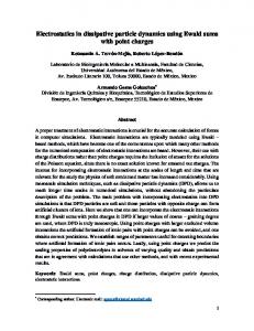
1 Introduction Dissipative Particle Dynamics (DPD) is already a well stablished simulation method to study particle systems[1]. In the seminal work by Hoogerbrugge and Koelman[2] the motivation of developing DPD was studying hydrodynamic behavior with a particle based method and an integration scheme very similar to that of Molecular Dynamics (MD). While theoretically, hydrodynamic conditions could be studied with MD, in practice, performing a simulation with the typical time step of MD for a big enough number of particles, such that the Reynolds number of a fluid can be varied considerably, would be prohibitely expensive in computer time, even with current computer systems. Additionally, most of the thermostats which would allow for an isothermal simulation in presence of flow, perturbe hydrodynamic correlation between particles. DPD tackled these two drawbacks to allow particle-based simulations in a scheme very similar to MD. As originally deviced[2], DPD allows for a higher time step than usual MD simulations. This was achieved by definining the so-called “soft potentials” as the interaction model between particles in the original DPD scheme. These linearly decaying potentials, have constant and small derivatives (forces), as compared to a typical interaction potential of MD simulation, such as the Lennard-Jones potential. The equations of motion of these “fluid particles” interacting with soft potentials can be integrated with a time step with a factor of 10 to 100 times higher than that used for the Lennard-Jones potential. This speed-up allows for the simulation of larger systems, and therefore higher Reynolds numbers. The other important contribution of DPD to the simulation of hydrodynamic phenomena is the use of a thermostat that conserves locally linear and angular momentum, which is one of the assumptions of the hydrodynamic continuum formulation of the equations of motion. Either locally or globally, most of the widely used thermostats in MD, such as Andersen, NoséHoover[1] or Langevin[3] thermostats, violate Galilean invariance and momentum conservation, giving rise to screening[4] or other alterations of hydrodynamic correlations. The DPD method solves this by stablishing a thermostatic process similar to Brownian Dynamics, in which a dissipative and a viscous forces are applied over the particles of the fluid. The difference is, however, that in the DPD method these forces are applied in a pair-wise form, and in the direction of the line that connects a pair of particles (see Fig. 1). In this way, the total “external force” on the particles is zero, resulting in local momentum conservation. Additional details will be given in section 2. We can mention other two appealing features of DPD. It can be implemented from a straight-forward modification of a working MD program, from which efficient parallellization strategies have been deviced[5, 6]. Additionally, it has a great versatility to study complex fluids or other soft matter systems in hydrodynamics context by adding interactions among particles, for example, harmonic or other spring-like interactions (bonded), to describe polymers, colloids or amphiphilic molecules[7, 1]. Also liquid mixtures can be studied, by changing the potential among different kind of particles.

Short form of title

3

While the original DPD method was thought as a complete simulation procedure, including the soft potentials and the pair-wise thermostat, it was soon realized that they do not need to be used together[4, 8]. One could use a DPD thermostat with any interaction model (potentials) among particles or molecules, and not only with soft potentials. This option of using “hard potentials”, such as Lennard-Jones or any other common potential in MD simulations comes, of course, at the price of reducing the time step in the simulations, which is one of the original advantages of DPD. However, the correct description of hydrodynamics can be a highly desirable feature in many physical situations of interest. In this work we review the use of the DPD method with soft and hard potentials for complex fluids and polymeric systems. In section 2, we review the DPD method as a variation of standard MD and Brownian Dynamics simulations. In section 3, we provide details of the use of soft and hard potentials to simulate soft matter systems such as polymeric systems. In this section we also provide a various examples of equilibrium DPD simulations with soft potentials. We devote section 4 to give examples of the use of DPD in soft matter systems under flow, to study the behavior and coupling of these soft matter systems under non-equilibrium conditions. We also show some difficulties as regards temperature conservation in strongly out-ofequilibrium simulations and how to deal with them in section 5. We provide the final comments and conclusions in section 6.

2 Details of the Dissipative Particle Dynamics method 2.1 Basic Molecular Dynamics simulation The DPD simulation scheme can be thought as an extension of the typical Molecular Dynamics algorithm[7, 1]. The basic idea in MD is integrating numerically the classical equations of motion, of a set of N particles. The Newton equations for each particle i is −

∂ V (r) ≡ fi =mi r¨i , ∂ ri

(1)

where mi is the mass of the particle, fi is the total force on particle i due to other particles of the system and any external field applied. In a simple bulk simulation, the evoution is done in a box of a certain volume and periodic boundary conditions must be imposed, to warrant that all the particles will be always in the simulation box. From a physical point of view, this bulk simulation should avoid any surface effect[1]. Assuming ergodicity, a time average over the integrated numerical trajectory of the N-particle system of any quantity depending on the dynamical variables positions {ri } and velocities{vi } is equivalent to an ensemble average

4

Short form of author list

hAiens ≡

1 τ

ˆ

τ 0

A({ri (t), vi (t)})dt,

where A stands for any physical quantity, function of the dynamics variables of the system. From the point of view of the statistical mechanics, integrating simply Newton equations corresponds to a micro-canonical ensemble in which the number of particles N, the volume of the system V and the total internal energy of the system E are held constant.

2.2 Simulating at constant temperature: Langevin thermostat The microcanonical ensemble, while useful theoretically is not usually used in experiments in which exchange of heat, particles and or volume is usually the case. A typical ensemble in experiments and, because of that, widely used in simulations, is the canonical ensemble, in which the constant thermodynamic variables are the number of particles N, the volume V and the temperature T . Keeping the temperature constant, means of course fluctuations of the energy of the system due to a heat exchange with a “thermal bath”. To simulate the system at constant temperature, some addition must be done to the original dynamical equations 1. In the last thirty years, significant effort has been done to extend the Newton equations of a classical system to obtain constant temperature. The different thermostats can be classified conceptually as those which provide constant temperature by stochastic relaxation (i.e Langevin thermostat or Brownian dynamics simulations ), stochastic coupling (Andersen thermostat), extended langrangian schemes (i.e. Nosé-Hoover thermostat), temperature constraining (Woodcock and Hoover-Evans thermostats) and weak coupling (Berendsen thermostat)[3]. All these schemes have advantages and drawbacks and find areas of application according to the systems, physical conditions and phenomena to be addressed. We will not review this, and suggest the excelent review by Hünenberger[3] and the classical textbooks of MD simulations[1, 7, 9]. We will give some details of Langevin thermostat, also termed Brownian Dynamics, as a first step, to describe then the DPD thermostat. In this scheme instead of integrating the Newton equation of motion, a Langevin equation describes the dynamics of each particle of the simulation. The integration scheme and most of the MD program implemmentation remains exactly the same, except that two force terms are added to the conservative forces already present in MD simulations. The first order equations of motion for the particle i are pi , mi p˙i = Fc i + Fi D + Fi R , r˙i =

where ri and pi are the positions and momenta of the particles. Fc stands for all the conservative forces of the system, with arbitrary molecular complexity. These are called the molecular interaction model. The Langevin thermostat adds a dissipative

Short form of title

5

and a stochastic force to the conservative forces of the system. It can be rationalized by thinking that a particle is coupled to an implicit fluid, which acts as a thermal bath.[8] The dissipative force on particle i is given by Fi D = −γ vi , where γ is a friction coefficient fixed in the simulation, and vi is the velocity of the particle. The random force, FRi , is chosen such that it has zero mean value and its variance satisfies hFiRµ (t)FjRν (t 0 )i = σi2 δi j δµν δ (t − t 0 ) ,

(2)

where σi is the noise strength. The relation σi2 = kB T γ /mi , couples the friction γ and the noise strength σi in a particular way such that the fluctuation-dissipation theorem is satisfied and the system is simulated in the canonical ensemble (NV T ). An elegant derivation of this can be obtained from a Fokker-Planck equation for this system[10]. This way of thermostating, also known as Stochastic Dynamics, allows particle simulations at constant temperature. However, this algorithm violates Galilean invariance, because it dampens the absolute velocities of the particles, thus assuming as “special” the laboratory frame. Langevin thermostat, while allowing the simulation of correct thermodynamic conditions is of little use for hydrodynamic phenomena. Taking a simple liquid, it was shown by Dünweg[11, 10], that this unphysical behavior can be thought as a screening length for the hydrodynamic correlations · ¸1/2 η ξ= , ργ /m where η is the viscosity of the fluid, ρ the number density, γ the friction constant and m the mass of each particle[11]. The propagation of momentum is screened and dampened, as compared to the correct hydrodynamics behavior.

2.3 The Dissipative Particle Dynamics thermostat The Dissipative Particle Dynamics thermostat improves Langevin thermostat and solves the screening problem. In this way allows to simulate hydrodynamics phenomena at the mesoscale in equilibrium and in presence of flows. It is very similar to the Langevin thermostat, described in the previous section. Dissipative and stochastic forces are applied, but to pairs of particles. The thermostat is also Galilean invariant, because dampens relative velocities and not the absolute velocity of a single particle. The stochastic forces are applied also to pairs of interacting particles in opposite direction, such that Newton’s third law is satisfied. In this was the total “thermostating” (external and non-conservative) force to a pair of particles is 0 and the momentum is conserved locally. The new expressions, for the dissipative and random forces are

6

Short form of author list

Fi D =

∑

D D FD ri j · vi j )ˆri j i j ; Fi j = −γω (ri j )(ˆ

∑

FRi j ; FRi j = σR ω R (ri j )θi j rˆ i j ,

j(6=i) R

Fi =

(3)

j(6=i)

where ri j ≡ ri − r j = ri j rˆi j and vi j ≡ vi − v j are the relative positions and velocities, respectively. γ is the friction constant, and σ the noise strength. Friction and noise, obey the relation σR2 = 2kB T γ , exactly in the same of way that Langevin thermostat. ω D (ri j ) and ω R (ri j ) are weight functions, that have to satisfy also a relation, to fullfill the fluctuation-dissipation theorem[12, 13]: [ω R ]2 = ω D .

(4)

θi j stands for a random variable with zero mean and second moment 0

0

hθi j (t)θkl (t )i = (δik δ jl + δil δ jk )δ (t − t ). The standard weight functions found in the literature are: ( (1 − r/rc )2 , r < rc [ω R ]2 = ω D = 0, r ≥ rc

,

(5)

(6)

where rc is the cut-off radius for a given molecular model. It is emphasized that Eq. (6) is just the typical choice when the DPD thermostat is employed in conjunction with “soft” potentials. Any choice satisfying Eq. 6 would be a suitable option for the weight functions. In Fig. 1 we present a sketch with the direction of the dissipative and stochastic forces of the DPD thermostat on a pair of fluid particles.

F

R

F

D

F

D

F

R

Fig. 1 Sketch of the dissipative and stochastic forces applied in a pair of fluid particles in the DPD thermostat. The forces are applied in the direction connecting both particles in such a way that the addition of all the “thermostating” forces vanishes.

Short form of title

7

3 Interaction models: Soft and hard potentials 3.1 DPD with soft potentials From the very inception of the DPD method[2], the spatial dependence of the conservative force (FCij ) was chosen as a short range, linearly decaying function: FCij = ai j (1 −

ri j )ˆeij Rc

(7)

where ri j = ri − r j is the relative position vector, eˆ i j is the unit vector in the direction of ri j , with ri being the position of particle i. The constant ai j , is the strength of the conservative force between particles i and j; Rc is a cut off distance. This force becomes zero for ri j > Rc . It should be remarked that this choice of distance dependent force is not arbitrary, as it has been shown to arise from properly averaged, microscopic interactions, such as the Lennard-Jones potential[14]. As for the interaction constant, ai j , Groot and Warren[15] have provided a guide to calculate it using the Flory-Huggins model for like-unlike particles, and the isothermal compressibility of water for like-like interactions. The standard procedure to choose the conservative force parameter for particles of the same type, aii , is given by aii = [

κ −1 Nm−1 ]kB T 2αρ

(8)

where Nm is the coarse-graining degree (number of water molecules grouped in a DPD particle), α = 0.101 is a numerical constant, ρ is the DPD number density and κ is the dimensionless compressibility of the system. It is defined by κ −1 = 1/(ρ0 kB T κT ) , where ρ0 is the number density of molecules and κT = (∂ p/∂ ρ0 )T is the usual isothermal compressibility. When one chooses a coarse-graining degree equal to 3 water molecules in a DPD particle and the water compressibility under standard conditions, κ −1 ' 16, the DPD force parameter takes the value aii = 78.3. The parameter for different types of particles, ai j , is calculated from the FloryHuggins coefficient χi j using the following relation: ai j = aii + 3.27χi j

(9)

The χi j value can be obtained from the solubility parameters. The remaining forces of the model, namely the dissipative force and the random force, are exactly as defined in Eq. 3. Because all the conservative forces are repulsive, the equation of state of DPD is positive definite and it does not have a van der Waals loop [15], therefore it cannot predict liquid-vapor phase transitions. However, this limitation can be overcome by introducing a local density dependent attractive term into the conservative force, equation 7, which is useful for predicting surface tension, see for example Ref. [16]. Among the advantages of the soft potentials used in DPD is the fact that finite size effects are minimal when the appropriate ensemble is used because the potentials are also short ranged [17]. This allows one to perform accurate

8

Short form of author list

simulations using relatively small, computationally inexpensive systems, as shown in Fig. 2

Fig. 2 Dependence of the interfacial tension γ ∗ between two immiscible model fluids as a function of the size of the simulation box. Notice how the difference between the values of the interfacial tension for the smallest and biggest boxes amounts to about 1%. The axes are drawn in reduced DPD units. Adapted from reference [17].

3.2 Selected examples of soft matter systems in equilibrium We provide in this section examples of DPD with soft potentials for equilibrium simulations. When beads are joined through a harmonic potential polymer chains can easily be simulated, as well as other types of molecules such as surfactants, rheology modifiers and others[15]. The influence of the characteristics of the harmonic force forming surfactant molecules on the interfacial tension between two immiscible liquids has been studied thoroughly [18] and it was shown that the predictions follow closely the experimental trends. Most applications of DPD have been carried out at constant temperature although there are plenty of situations of importance for modern research where the influence of temperature is not sufficiently well understood. One of such cases is the dependence on temperature of the interfacial tension between liquids. Very recently, an extension of the DPD model that incorporates the variability of the temperature has been proposed[19]. It is based on the introduction of the temperature dependence of the solubility parameters for the pure components in a mixture, which leads to temperature dependent interaction parameters, see equations 8 and 9. Applying the temperature dependent form of DPD to the in-

Short form of title

9

terfacial tension between organic solvents and water led to predictions that are in excellent agreement with experimental results[19]. Another important extension of the DPD model is the incorporation of electrostatic interactions through the method of the Ewald sums. Using distributions of charge instead of point charges to avoid the formation of artificial ionic pairs, the behavior of poly-electrolytes in solution under the influence of varying ionic strength has been predicted and compared with similar studies carried out with certain proteins[20]. In particular, it has been shown that strongly charged poly electrolytes in aqueous solution experience a contraction followed by a re-expansion as a function of the tetravalent salt content, as shown in Fig. 3.

Fig. 3 The squared radius of gyration Rg of a poly-electrolyte made up of 32 equally charged monomers, in aqueous solution with varying ionic strength Cs . The latter is made up of tetravalent ions of Na neutralized with Cl ions. The axes are drawn in reduced DPD units. Adapted from reference[20] .

The contraction-re-expansion behavior quantified through the radius of gyration Rg of a model poly electrolyte shown in Fig. 3 is the result of a complex interplay between the electrostatic interaction and the excluded volume effect brought about by the softness of the DPD interaction potential. Moreover, it is by no means an artifact of the DPD model, as it has been obtained using other interaction potentials and has also been observed in experiments with proteins in aqueous solution [21]. In fact, using this electrostatic version of DPD it has been possible to predict the scaling exponent of the radius of gyration, defined by the well known relation Rg ∼ N ν where N is the polymerization degree and ν is the scaling exponent[20]. It is known that depends on the quality of the solvent in which the polymer is immersed, and on the dimensional of the system. For neutral polymers in good solvent it has been known for some time now that ν = 0.588. However, for poly-electrolytes much less is known. To begin with, it is not even firmly established if a scaling relation is obeyed, much less what the value of the scaling exponent should be. Nevertheless,

10

Short form of author list

several groups have shown that poly-electrolytes do show scaling characteristics in their radius of gyration, but their scaling exponent is usually larger that its counterpart for neutral polymers.

Fig. 4 The scaling exponent of the radius of gyration as a function of the polymerization degree, under a varying concentration of Na and Cl ions. The y – axis is dimensionless while the x – axis is shown in reduced DPD units. Adapted from reference [20].

Figure 4 shows the values of the scaling exponent of the radius of gyration for model linear poly-electrolytes of different polymerization degrees as a function of the ionic strength. The values of the scaling exponent are well above the 0.588 neutral polymer value in good solvent, although the results shown in Fig. 4 were obtained for simulations in which all the interaction parameters (see equation 8) between the poly-electrolyte and solvent were kept the same. These conditions correspond, in the neutral case, to the so-called theta solvent, therefore the results shown in Fig. 4 demonstrate that the quality of the solvent can be strongly modified by the electrostatic interactions.

3.3 DPD with hard potentials As regards the use of DPD with hard potentials, we mention a widely used polymer coarse-grained model, developed by Kremer and Grest[22, 23]. It has been applied to a variety of thermodynamic conditions and physical systems as glasses, polymer melts and solutions, and polymer brushes [24, 25, 26, 27, 28]. The bonded interaction along the same polymer is modeled by a finite extensible non-linear elastic (FENE) potential:

Short form of title

11

·  ³ ´ ¸ − 1 k R2 ln 1 − r 2 r ≤ R0 0 2 R0 UFENE = ,  ∞ r > R0

(10)

where the maximum allowed bond length is R0 = 1.5σ , the spring constant is k = 30ε /σ 2 , and r = |ri − r j | denotes the distance between neighboring monomers. Excluded volume interactions at short distances and van-der-Waals attractions between beads are described by a truncated and shifted Lennard-Jones (LJ) potential: U(r) = ULJ (r) −ULJ (rc ) ,

(11)

with ULJ (r) = 4ε

·³ ´ σ 12 r

−

³ σ ´6 ¸ r

,

(12)

where the LJ parameters, ε = 1 and σ = 1, define the units of energy and length, respectively. The temperature is therefore given in units of ε /kB , with kB the Boltzmann constant. ULJ (rc ) is the LJ potential evaluated at the cut-off radius. There are typically two values taken as cut-off distance: (i) the minimum of the LJ potential rc = 21/6 σ ' 1.12σ and (ii) twice the minimum of the LJ potential: 1 rc = 2 × 2 6 σ ' 2.24σ , which allows to consider poor solvent conditions. In the first case, the interactions between monomers of different chains are purely repulsive. From a point of view of polymer solutions, this means good solvent conditions because the polymer bead favors to be close to the solvent, giving rise to an effective repulsion among polymer beads. In the second case, longer ranged attractions are included (full Lennard-Jones potential), giving rise to liquid-vapor phase separation and droplet formation[29, 30, 31], for the adequate thermodynamic conditions.

4 Selected examples of DPD in flow simulations 4.1 Polymer Brushes with soft potentials There are a number of applications in soft matter systems that require of surfaces covered by polymers to improve factors such as colloidal stability, reduction of interfacial tension for wetting purposes, or improvement of lubrication. The most common procedure to accomplish this is by grafting polymer chains of varying length to surfaces, changing the grafting density also. Within the context of computer simulations, when one is dealing with systems that model colloidal dispersions or surfaces with grafted polymers, to ensure that the confined system is in chemical, mechanical and thermal equilibrium with the non – confined fluid it is necessary to use the so-called Grand Canonical ensemble, which is well known in statistical mechanics, and requires that the chemical potential, the volume of the system and the temperature be fixed during the simulation. To do so one needs to perform Monte Carlo

12

Short form of author list

simulations, which are relatively demanding from the computational point of view because the number of particles in the simulation box is fluctuating and, as the concentration is increased, the probability of introducing new particles into the system becomes exceedingly small. However, for moderate densities it has been shown to be a very useful tool. Within the context of DPD there are now some works that have explored the properties of fluids confined by surfaces, covered with polymers, using the Monte Carlo method in the Grand Canonical ensemble (MCGC). A common approximation consists of substituting the colloidal particles by planar surfaces, given the disparity of sizes between them and the solvent molecules. Also, planar surfaces are useful to model pores or mimic experimental arrangements such as that of the atomic force microscope or the surface force apparatus[32]. These planar walls have been implemented in DPD through two methods: either by fixing in space some layers of DPD particles, placed at the ends of the simulation box [33], or by introducing an effective wall potential that acts on particles close to the ends of the simulation box [34]. Several models for the wall potential have been proposed; the first one being a linearly decaying force, in the spirit of the other DPD forces, namely[34]: Fi (z) = aw,i (1 −

z )ˆz zc

(13)

Equation 13 represents the force that acts on the ith-particle in the zˆ direction (perpendicular to the plane where the surfaces are placed), aw,i is the interaction strength of such force, and zc is a cutoff distance, beyond which the force becomes identically zero. For obvious reasons, this model is usually called the “DPD wall” force. Recently a self-consistent surface force was obtained for DPD particles [35]. It considers an infinite planar wall made up of regularly spaced, identical DPD particles that interact with other particles on the wall and with particles in the fluid through the usual DPD conservative force (see equation 7 and Fig. 4). By integrating the contribution to the total wall force from each particle on the surface it is possible to obtain an exact expression for the effective DPD surface force, which is given by the following polynomial [35]: " µ ¶ µ ¶4 # µ ¶3 z 2 z z Fi (z) = aw,i 1 − 6 −3 zˆ (14) +8 zc zc zc where the symbols have the same meaning as in equation 13, except that the strength of the interaction is given in this case by the relation:

π ρw R3c ai j . (15) 12 In equation 15 ρw is the density of the wall, Rc is the usual cutoff radius, and ai j is the conservative force strength, equation 7, between the particle i in the fluid and j on the wall. The surface force in equation 14 is appealing for several reasons: it is exact, it is soft and short – ranged as the other DPD forces, and its strength is defined through the interaction strength of the conservative force as expressed in equation 15. Using this effective surface force, GCMC simulations have been performed to aw,i =

Short form of title

13

Fig. 5 Model to derive an effective, DPD surface force (left). The resulting force is a polynomial (see equation 14) which is also of short range, as are the other forces that make up the DPD model (right). Adapted from reference [35].

calculate the full solvation force that the walls exert on a simple monomeric DPD fluid. This solvation force, which is equal to the change in the free energy of the system between two compression states, per unit area, is surprisingly of relatively long range, as shown in Fig. 5, even though the surface – fluid particle force is of short range. This phenomenon is the result of the collective many – body interactions that carry information about the boundary conditions of the fluid in the direction of the confinement.

Fig. 6 (color online) The exact DPD wall-fluid force (equation 6) is shown in blue, while the full, many-body solvation force obtained from simulations with the wall force is shown in red squares. Both scales on the y-axis are shown in reduced DPD units, as is also the x-axis. To convert the latter into physical distances it is necessary to multiply z∗ by 6.46Å. Adapted from reference [35].

14

Short form of author list

By attaching polymer chains to these effective surfaces it is possible to calculate the force between colloidal particles covered with polymer brushes and compare it with other models, like the well known Alexander-de Gennes (AdG) model[36, 37], which is based on scaling arguments, and assumes that the density profile of the monomers that make up the polymer brushes is a step function. This is known to be inaccurate. It also assumes that the polymer chains do not interact with one another, and that they are immersed in a solvent of good quality [36, 37]. The AdG force is then the result of short range repulsion caused by the increased osmotic pressure when the polymer brushes are brought into close contact, and elastic attraction created by the entanglement of polymer chains on opposite brushes. In the left panel of Fig. 7 we present the density profile of the polymer brushes at a given separation between the walls, which shows the beads attached to each surface and the structuring in the density profile of the brushes, which is a consequence of having relatively short chains (N = 5 for the case shown in this figure). Notice how this profile is far from looking like a step function. Yet, as shown in the right panel of Fig. 7, the AdG model reproduces fairly well the trend in the full solvation force obtained with GCMC DPD simulations, although the latter are more accurate because the interactions between all particles are accounted for.

Fig. 7 Density profile for polymer chains with degree of polymerization N = 5 (left). The inset shows an image from the actual simulations. Full solvation force obtained from GCMC DPD simulations of polymer brushes (right). The line represents the AdG model. Axes are shown in reduced units. Adapted from reference [35].

The disjoining pressure of a simple monomeric fluid confined by effective linearly decaying wall forces, as the one shown in equation (4), has been calculated by means of GCMC-DPD simulations. This is a quantity of importance when studying the properties of confined fluids because it is a measure of the stability of complex fluids under confinement under fixed chemical potential[34]. It is defined as the difference between the pressure tensor component in the direction perpendicular to the confinement (PN ) and the pressure of the bulk (unconfined) fluid, PB . In Fig. 7 we see the disjoining pressure (Π ) as a function of the distance between the walls (Lz ), for a monomeric fluid confined by linearly decaying surface forces. There appear intercalated maxima with minima whose interpretation is the following. The maxima

Short form of title

15

in Π represent thermodynamic states with maximal force between colloidal particles (per unit area) represented by the walls, mediated by the corpuscular nature of the solvent. This maxima are the consequence of an ordered array of the solvent molecules into layers, whose order gets increasingly lost as the separation between the surfaces grows, as should be expected. These states correspond to conditions of optimal stability for the colloidal dispersion. The minima seen in Fig. 8 represent states where there is an attractive (negative) force between the surfaces, therefore they are thermodynamically unstable and would lead to the agglomeration of colloidal particles. It is remarkable that an attractive force can emerge from a model (DPD) where all particle interactions are repulsive, including the wall force, and it occurs because of the confinement condition and the corpuscular nature of the solvent, which forces the particles to form orderly layers when the force is at a maximum (see points labeled a, c and e in Fig. 8) and be disordered when the force is minimal (as in states labeled b and d in Fig. 8).

Fig. 8 The disjoining pressure Π of a simple fluid made up of monomers obtained from GCMC–DPD simulations of the fluid confined by linearly decaying wall forces, as a function of the distance separating the surfaces. The inset show a schematic diagram of the system and how is calculated. The top part of the figure illustrates how the maxima and the minima in are due to the arrangement of the fluid’s molecules. The axes are shown in reduced units. Adapted from reference [34].

The behavior shown in Fig. 8 reproduces very well the trends found in experiments and with other calculation methods[32], and lends credence to the usefulness of DPD as a precise predicting tool, not only for polymers in solution, but also for confined complex fluids. It is advantageous to perform simulations like these before embarking in laborious, time consuming and expensive experiments, such as those required to determine adsorption isotherms. In the design of new colloidal dispersions for the paint industry, for example, or for the improvement and optimization of known formulations, it is usually required to determine the amount of material

16

Short form of author list

(polymers, surfactants) that needs to get adsorbed on the surfaces of the colloidal particles. This is traditionally determined from adsorption isotherms, which can take several weeks to measure and interpret. By contrast, the adaptability of computer simulations allows one to calculate adsorption isotherms in relatively short time, having full control of the thermodynamic variables. For these purposes it is crucial to perform the calculations at constant chemical potential (and volume and temperature). Because of the mesoscopic reach of the DPD model and its success in predicting the behavior of polymers in solution and also confined fluids, it becomes a well suited tool for the study of adsorption of polymers on colloidal particles.

Fig. 9 Adsorption isotherms obtained with GCMC–DPD simulations of fluids confined by a Lennard-Jones (9 − 3) surface model (left), and a linearly decaying, DPD wall force (right). The fluid is made up of the monomeric solvent and a varying number of linear polymer chains (N = 7) to represent PEG molecules. Red circles represent the simulation results while the blue squares are the experimental data, taken from reference. The axes are normalized with their maximum value so that both scales range from 0 to 1. The lines are only guides for the eye. Adapted from reference [12].

Figure 9 shows adsorption isotherms obtained with GCMC – DPD simulations for two cases, one where the surfaces were implemented as Lennard-Jones (9-3) forces, to represent alumina surfaces (Al2 O3 ) that are known to have hydrophilic character [38]. In the other, the walls were modeled as soft DPD walls (see equation 13), meant to represent the hydrophobic nature of silica (SiO2 ) surfaces. The fluid confined by these walls is composed of solvent monomers and a varying number of PEG molecules, which are modeled as linear chains with N = 7 beads each, joined by harmonic springs. This polymerization degree corresponds to a molecular weight Mw = 400 for PEG [34]. The predicted adsorption isotherms are compared with the experimental counterparts [38] in Fig. 9. Notice how the DPD methodology correctly reproduces the trends if not the actual values of the isotherms; not only that, it is possible to model different surfaces characteristics by a judicious choice of the wall force model or interaction parameters. Up to this point all the results reported for confined fluids were carried out for neutral systems. However, polyelectrolytes which are charged polymers are ubiquitous in nature and in modern day applications[39]. Many colloids acquire electric charges on their surface when immersed in a polar solvent, like water, and are rich in showing complex phenomena when they are subject to varying ionic strength and pH, as polyelectrolytes are as well. And from the point of view of fundamental research, the long range nature

Short form of title

17

of the Coulomb interaction gives rise to behavior that is qualitatively different from neutral systems, which needs to be thoroughly investigated to reach a satisfactory understanding of soft condensed matter systems. Because of these needs it became necessary to adapt the DPD model so that it could handle long range interactions such as the electrostatic one, for confined systems. The natural route was to adapt the Ewald sums method for cases when there is reduced symmetry, as in the confined fluids we have discussed [40].

Fig. 10 Fully charged linear cationic polyelectrolyte on neutral surfaces with N = 7 beads. Only every other bead is charged. In the left panel are shown the adsorption isotherms obtained at three different pH values. The symbols represent the results of the simulations while the solid lines are the best fits to the Langmuir adsorption isotherm model. In the right panel of this figure we show the full force between colloidal surfaces mediated by the polyelectrolytes and the solvent, at the same pH values as in the left panel. Notice that when the pH is increased so is the surface force, in contrast with the adsorption isotherm trend. The axes in the left figure are shown in reduced DPD units while those of the figure in the right have been appropriately dimensionalized. Adapted from reference [40].

Alarcón and co-workers [40] calculated the first adsorption isotherms of polyelectrolytes using the GCMC–DPD algorithm adapted with Ewald sums for confined systems as a function of pH. They studied the adsorption of weakly charged, linear cationic and anionic polyelectrolytes at various values of pH on negatively charged and neutral colloidal surfaces. The adsorption isotherms they obtained for cationic polyelectrolytes adsorbed on neutral surfaces modeled by the exact, selfconsistent DPD wall force (equation 14) are shown in the left panel of Fig. 10. For the model polyelectrolyte used in those simulations the adsorption increases as the pH is reduced, which was attributed to the competition between the polyelectrolytes and their counterions for the adsorption sites on the colloids surfaces, because when the adsorption of the counterions grows when that of the polyelectrolytes is reduced. This is precisely the trend found in experiments performed on comparable situations [41]. The right panel in Fig. 10 shows the full surface force that neutral colloidal particles, modeled by the exact DPD wall force, exert on each other by means of the cationic polyelectrolytes at different pH values [40]. This is the first calculation of its kind, not only within the context of DPD simulations. The trend found in the surface force is entirely different from that found in the adsorption isotherms (left panel in the same figure) even though the calculations were performed on the same systems. In other words, when the pH of the cationic polyelectrolyte is increased,

18

Short form of author list

it translates into a larger surface force between colloidal particles. What this means is that if one is looking for optimal stability of colloidal dispersions it may be advantageous to add less polyelectrolytes as dispersants, at a basic pH, because the competition of electrostatic interactions between polyelectrolytes and counterions, and the excluded volume interactions with the solvent are enough to increase the many-body surface force so that the colloidal dispersion turns out to be optimally stable, as the right panel of Fig. 10 shows. The results shown in the right panel of Fig. 10 fully reproduce experiments carried out on polyelectrolytes and characterized using atomic force microscopy at different pH [41], among others. Lastly, we comment on some very recent DPD simulations that model complex fluids under stationary flow using soft DPD potentials. The reason for simulations of this type stems from the need to understand phenomena seen in applications such as drug–carrying liposomes in the pharmacological industry, in the processes of enhanced oil recovery, for the design of improved rheology modifiers in the paint industry, as well as lubricants, to mention a few. The idea behind non equilibrium, stationary flow simulations for applications like those mentioned above is as follows: two parallel plates are placed a certain distance apart, say in the z–direction; then a constant force is applied to the top plate and an equal in magnitude but opposite in direction force is applied to the bottom plate. This creates a velocity gradient (or shear rate) which is responsible for creating a steady flow known as Couette flow. We shall have more to say about the details of this type of flow in the next section, but for now we focus on the use of soft DPD potentials in non-equilibrium simulations. Although many works have been published that use computer simulations to study Couette flow, most of them have been carried out using microscopic models, which are accurate but are very time-consuming, more so that equilibrium simulations. Recently, a study of the rheological properties of polymer brushes under theta solvent conditions using only soft DPD interactions has been published [42]. The system consists of two parallel plates on the xy−plane, modeled as soft DPD wall forces, see equation 13, separated by a fixed distance D, where a number of polymer chains were grafted at one of their ends and at grafting densities large enough to form polymer brushes. A constant velocity v0 is applied to the grafted ends of the polymer chains on the top and bottom plates, in opposite directions, so that stationary flow is produced by the collisions of the chains with themselves and with the solvent particles. This fives rise to a mean constant force Fx in each plate, in the stationary regime. The grafted beads on the surfaces move with a constant velocity (v0 ) but there is a velocity gradient of constant shear rate γ˙ along the direction separating the plates. Figure 11 shows a configuration of this system, extracted directly from the simulations. One can calculate rheology properties such as the viscosity η for fluids under flow, as the one shown in Fig. 11, using the following relation [43, 44]:

η=

hFx (γ˙)i/A . γ˙

(16)

In equation 16 Fx is the magnitude of the constant force in the x-direction, applied to the planar surfaces of area A and γ˙ is the shear rate. The brackets represent an av-

Short form of title

19

Fig. 11 (color online) A system configuration extracted directly from non-equilibrium computer simulations using soft DPD interactions of polymer brushes grafted on soft DPD surfaces. The blue particles are the grafted beads which move at constant speed v0 in the direction indicated by the arrows. Those beads drag the rest of the beads forming the polymer chains (in yellow) to produce flow of the solvent particles (in red). The green line indicates the velocity gradient as is expected in stationary Couette flow. Adapted from reference [42].

erage over the entire simulation time [42, 44]. By changing the applied force one can vary the shear rate and then measure the dynamic response of the fluid through the viscosity using equation 16. Newtonian fluids are characterized by viscosities that are independent of the shear rate, but most fluids of interests for modern applications, and the fluid simulated and shown in Fig. 11 are of the non-Newtonian type, namely, they have viscosities that are shear rate dependent[43]. Another rheological property of interest for polymer brushes is the friction coefficient between the brushes and the fluid, which is given by the following expression:

µ=

hFx (γ˙)i , hFz (γ˙)i

(17)

where hFx (γ˙)i and hFz (γ˙)i represent the mean forces that the grafted beads experience along the direction of the flow (x) ˆ and perpendicularly to it (ˆz), respectively. The brackets symbolize time average over all the particles in the simulation box. Clearly, is a dimensionless number. Figure 12 shows the predictions for the viscosity and the friction coefficient obtained from DPD simulations of Couette flow for linear polymer brushes of varying polymerization degree under theta solvent conditions, using equations 16 and 17, respectively[42]. In particular, the viscosity (left panel in Fig. 12) shows what is usually known as “shear thinning”, i. e., the viscosity is reduced as the shear rate is increased. As is seen in the figure, the viscosity for brushes of different polymerization degrees N, obeys a universal law for large values of the shear rate. In fact, a scaling law can be extracted, yielding η ∼ γ˙−0.31 independently of the value of N. On the other hand, the friction coefficient (right panel in Fig. 12) increases with the shear rate but obeys also a scaling law, which is found to be µ ∼ γ˙0.69 . These scaling exponents are in excellent agreement with those predicted using different arguments [45] and they are found to be related according to those predictions [42]. To conclude this section, there are numerous examples where the application of the soft DPD potentials have yielded novel and accurate predictions which make of

20

Short form of author list

Fig. 12 (Left) Viscosity of the grafted beads of polymer chains forming brushes of three different polymerization degrees, as a function of the applied shear rate. To use dimensionless units on both axes, the y-axis was normalized with the limiting value of the viscosity at zero shear rate η0 . The x-axis was normalized with the value of the shear rate when the behavior of the applied force changes from linear to sub-linear, so defining the Weissenberg number We. The line is the predicted scaling law. (Right) The friction coefficient normalized by its value at the transition from linear to sublinear regimes, as a function of We. The friction coefficient for all brushes modeled obeys the scaling law µ /µ ∗ ∼ We0.69 . See text for details. Adapted from reference [42].

this model one of the leading current tools to understand phenomena in soft matter systems. Here we have reviewed only some of the recent ones, mostly taken from our own work and expertise.

4.2 Hard coarse-grained potentials In this section, we provide examples of simulations of flows with the coarse-grained Kremer-Grest model for polymers. The two simplest hydrodynamic flows can be easily set within the MD with DPD thermostat simulations. These two flows are very important to characterize the behavior in operational conditions of Microfluidic devices. The small size of the channels that confine the fluid, means usually a laminar regime, far away of the turbulent hydrodynamic regime. In these examples, the Couette (linear) flow is established by moving the walls of the polymer-coated channel at constant and opposite velocity. This builds up, at stationary regime, a linear velocity profile in the channel with 0 velocity exactly at the center of the channel. A typical simulation is shown in the inset of Fig. 13. The Figure shows a density profile with the two species in the system: a polymeric liquid of ten-bead chains (gray) which is confined between two layers of end-grafted polymers, a polymer brush (red). The densities show the brush-liquid interfaces clearly defined. The liquid is not able to enter in the brush layer, even when all the interactions are attractive, due to entropic effects[8, 46]. This is the well-known case of autophobicity[44]. The brush thickness, depends on the grafting density (number of chains per unit area grafted at the wall). This system can be studied in equilibrium and also under flow.

Short form of title

21

z x

center

0.6

-3

ρ(σ )

0.8

0.4

ρb ρm

0.2

0

7

8

9

10

11

z(σ) Fig. 13 Density profile of the brush (full line) and the melt (dashed-dotted line) for ρg = 0.77σ −2 . The inset shows a configuration of the simulated system, aligned with the density profile such that the brush-melt interface coincides. Adapted from Ref. [46] .

The velocity profiles obtained as a result of moving the wall at constant and opposite velocity are shown in Fig. 14. The linear velocity profiles are clearly observed for two different grafting densities in the brush (upper and lower panels). The density profile is also shown with open circles. Close to the brush-liquid interface, inside the brush layer, deviations from the dominant linear profiles are observed. This has a physical meaning, since the interface properties are not expected to be the same as that of the bulk liquid, in the center of the channel. The mixture of liquid and grafted chains (which do not flow in the wall reference frame), can be understood as an effective liquid of different viscosity, in this zone. It is important to emphasize the difference of this simulation scheme as compared to that, more common, in computational fluid dynamics. In MD with DPD, neither the viscosity of the fluid, nor the boundary conditions (i.e. slip length or slip velocity) are imposed to the system. These two quantities can be measured in the simulations for given flow, thermodynamic conditions and molecular interaction models. Figure 15 shows the Poiseuille-like velocity profile for the same system. It is obtained by applying a constant body force for each particle. This can be understood as a gravity force acting on each particle, or a pressure difference. Only the velocity profile of the polymeric liquid is shown. The brush has a vanishing mean velocity since the molecules are grafted to the hard substrate. The velocity profiles are progressively narrower upon increasing grafting density due to the increased thickness of the brush layer. This smaller effective width of the channel, reduces also the flow rate, at constant body force (or pressure gradient). The mean viscosity of the poly-

22

Short form of author list

2

vx(z)Re /(DwD)

12

5*ρmelt vw=0.06 vw=0.12 vw=1.00 vw=1.50 vw=1.75

*

ρ =13.40

10 8 6 4 2 0

2.5

3

3.5

2

vx(z)Re /(DwD)

12

4

4.5

5

*

ρ =35.10

10 8 6 4 2 0

3.5

4

4.5

5

z/Re Fig. 14 Velocity profile for the linear Couette flow simulations for different wall velocities (shear rate). The velocity is scaled with the dynamic scale of a polymer melt of the same density as the brush Dw D/R2e , where Dw is the channel width, D the diffusion coefficient of the equivalent polymer melt and Re its end-to-end distance. The open circles show the density profile of the same system. It should be noted that it is highly independent of the flow conditions. Adapted from Ref. [46] .

Short form of title

23

meric liquid can be extracted from the simulations, by fitting the analytic velocity profile obtained from the integration of the Navier-Stokes equation: v(z) =

ρ fx (z − z0 )(Dw − z0 − z) , 2η

(18)

where ρ is the number density of the fluid at bulk, fx = 0.008ε /σ is the external body force applied on each bead to produce the flow, Dw is the channel width and z0 indicates the position at which the velocity profile extrapolates to 0 velocity. The viscosity η , is the only parameter in Eq. 18 that is not measured directly from the simulation. It can be obtained from the fit of the profile with Eq. 18. These examples illustrate the use of DPD with hard potentials, in which the structural properties of the liquid, flow properties (slip length and slip velocity, velocity profile) and rheological properties (viscosity, regions of non-newtonian behavior) of these soft matter systems can be obtained from the simulations using the two simplest hydrodynamic flows, i.e Couette (linear) and Poiseuille (quadratic) flows. Velocity fields, together with density profiles can be studied globally[44, 46] , locally (for example inside a droplet)[31, 47, 48] or for a given type of molecule[49]. 1.25 *

ρg = 13.40

1

*

ρg = 17.95

0.75

*

ρg = 35.10 *

ρg = 43.80

2

v(z)Re /(DwD)

*

ρg = 27.10

0.5 0.25 0 2

2.5

3

4

3.5

4.5

5

5.5

z/Re Fig. 15 Symmetrized velocity profile for Poiseuille-flow simulations for different grafting densities. The body force acting in each bead is fx = 0.008ε /σ . The x-axis ˆ is given in units of a measure of the polymer size, the end-to-end radius for these liquid density and temperature is Re = 3.66σ . The channel width is D = 40σ with the center of the channel in 20σ (z/Re = 5.46). There the velocity profile reaches the maximum. Adapted from Ref. [46] .

24

Short form of author list

5 The conservation of temperature in flow simulations Under conditions of high flow, the DPD thermostat can have problems to maintain a constant temperature across the fluid[8]. A particular complicated case takes place for good solvent conditions in polymeric or other soft matter system. An important difference between Langevin and DPD thermostat, is that Langevin forces act on every particle, independently of the cut-off radius of the potential or the density of the system. DPD, however, acts on pairs of interacting particles, those that are within the cut-off radius. For systems with short cut-off radii as it is the case of the KremerGrest model for polymers in good solvent conditions, the number of thermostated pairs per time step can be pretty low, reducing the ability of the DPD thermostat to extract a given amount of heat per unit time in the system. This behavior is illustrated in Fig. 16 for Poiseuille-flow simulations. Panel (b) shows the velocity profile across the channel for different external forces. There is a quadratic behavior, but some deformation is observed, as compared to Fig. 15. The reason for that can be noticed in Fig. 16(a), which shows the temperature profile, across the channel. These are extracted from the mean quadratic velocity in the directions without flow (yˆ and zˆ). The equipartition theorem implies 12 mhv2y i = 12 kB T , from which a local temperature can be extracted. For higher forces, starting in fx = 0.014ε /σ , the temperature is not conserved and heating of the liquid occurs in the regions of higher shear rate. There, the heat production per unit time is higher than the maximum removed by the thermostat and the temperature cannot be maintained at the defined value kB T = 1.68ε . In these situations various strategies can be adopted to maintain the constant temperature. The simplest choice would be increasing the friction constant of the thermostat. This can be perfectly done if the short-time dynamics of the molecules is not of interest. This means also increasing the amplitude σR of the stochastic force (see Eq. 3). Another alternative is to change the weight functions in the forces of the thermostat. As it was emphasized, they only have to fulfill the requirement of Eq. 4 to warrant the fluctuation-dissipation theorem. Fig. 17 illustrates this option. It shows the temperature profile across the channel with exactly the same flow conditions for different weight functions. The usual choice (Eq. 6) has the worst performance with the higher deviation from the desired temperature kB T = 1.68ε . The usual choice of weight functions fail to keep constant temperature across the channel (dark full £ ¤2 line), while the constant weight functions ω D = ω R = Θ (Rc − r) gives much better temperature conservation. The defined temperature is shown with a dashed line. Constant weight functions, fulfill temperature conservation at the desired temperature. The last option that we comment here to improve temperature conservation is increasing the number of thermostated pairs of particles by extending the cut-off for the DPD forces. In this case, the√cut-off of the conservative forces continues to be short range, for example Rc =6 2σ (good solvent for Kremer-Grest model). But √ (DPD) the cut-off for DPD forces is twice as long: Rc = 2 ×6 2σ . This option was successfully employed in Ref. [49].

Short form of title

25 fx=0.008 fx=0.032 fx=0.014 fx=0.28 fx=0.45 fx=0.63

T (ε/kB)

6

(a)

4 2

(b)

vx (σ/τ)

10 8 6 4 2 0 0.2

0.4

z/D

0.6

0.8

Fig. 16 Upper panel: Temperature and velocity profiles for different external forces for a polymeric liquid of 10-bead chains confined in a brush coated channel. Lower panel: velocity profiles of the Poiseuille flow simulations for the same cases of the upper panel. For a high body force the temperature is not conserved across the channel, reaching the maximum deviation in the regions of highest shear rate (local velocity gradient). Adapted from Ref. [8].

This problem of temperature conservation shows up for hard potentials at very short cut-off radius and strong flow conditions. This by no means limit the use of DPD, taking into account the solutions we propose in this section.

6 Concluding remarks In this contribution we review the Dissipative Particle Dynamics method, as a useful simulation technique to study soft matter systems in equilibrium and under flow. We emphasize the role of DPD as a thermostat that takes into account correctly the hydrodynamic correlations in the system, unlike many thermostats used in molecu-

26

Short form of author list ωR=1-r/rc

(a)

ωR=(1-r/rc) ωR=const.

T(ε/kB)

2

1/2

1.9 1.8 1.7 1.6 0.2

0.4

z/D

0.6

0.8

Fig. 17 Temperature profile for different DPD weight functions in a Couette-flow simulation. The walls are moved at vw = 3σ /τ and the channel width is Dw = 30σ , with a shear rate of γ˙ = 0.3τ −1 . The usual choice of weight function fails to keep constant temperature across the channel (dark full £ ¤2 line). Constant weight functions ω R = ω D = Θ (Rc − r), are able to give a temperature profile at the defined temperature (dashed line). Θ is the Heaviside function and Rc the cut-off of the forces. Adapted from Ref. [8] .

lar dynamics. This is a desired property to study stationary flows at the mesoscopic level with coarse-grained models of the molecular degrees of freedom. We give examples of the use of the DPD thermostat with soft potentials and hard potentials for polymeric liquids, polymer brushes and simple liquids. In equilibrium simulations with soft potentials, we also illustrate the use of DPD with Coulomb interactions to model polyelectrolytes, confinement and constant chemical potential simulations in the grand-canonical ensemble (µ V T ). We show that DPD is suitable to generate simple flows like Couette and Poiseuille and have access to the main velocity of density fields, characteristic of hydrodynamic theories but also to the boundary conditions and dynamics coefficients such us diffusion coefficients or viscosity. The latter are not imposed to the system, but obtained from the simulation itself, for given molecular model and flow conditions. In the studied cases the goal is simulating the system at constant temperature, though DPD can be modified to perform energy-conserving simulations, to explore heat conduction[50, 51]. For some particular cases of very short-range potentials and strong flow conditions, the ability of DPD to keep the temperature at the fixed value must be verified. We report also some examples in which temperature is not conserved and the workarounds to follow when this is the case. We think that DPD is a powerful and efficient tool to simulate soft matter systems under flow, keeping the dynamics of the individual molecules. This can be exploited in fields where surface-to-volume ratio of the confined liquid or polymeric compound is not negligible and the effects of the interface are important for the whole properties of the system. This would be the case in Microfluidic devices, oilrecovery problems in porous media or biological interfaces and vascular systems.

Short form of title

27

Acknowledgements C. P. thanks Marcus Müller for the enjoyable and fruitful discussions since I started in this exciting topic of simulations of soft matter systems. Kurt Binder and Torsten Kreer are also gratefully acknowledged for the support and scientific discussions in the nice times of Mainz. A. G. G. would like to thank F. Alarcón, A. Balderas Altamirano, C. Carmín, E. Mayoral, and E. Pérez for their help and collaborative efforts

References 1. D. Frenkel, B. Smit. Understanding Molecular Simulation: From Algorithms to Applications. Academic Press, 2002. 2. P. J. Hoogerbrugge, J. M. V. Koelman. Simulating microscopic hydrodynamic phenomena with dissipative particle dynamics. Europhys. Lett., 19:155, 1992. 3. P.H. Hünenberger. Thermostat algorithms for molecular simulations. Adv. Polym. Sci., 173:105, 2005. 4. T. Soddemann, B. Dünweg, K. Kremer. Dissipative particle dynamics: a useful thermostat for equilibrium and nonequilibrium molecular dynamics simulations. Phys. Rev. E, 68:046702, 2003. 5. S.J. Plimpton. Fast parallel algorithms for short-range molecular dynamics. J. Comp. Phys., 117:1–19, 1995. 6. W. Michael Brown, Axel Kohlmeyer, Steven J. Plimpton, Arnold N. Tharrington. Implementing molecular dynamics on hybrid high performance computers-particle-particle particlemesh. Computer Physics Communications, 183(3):449 – 459, 2012. 7. M. P. Allen, D. J. Tildesley. Computer Simulations of Liquids. Clarendom Press, Oxford, 1987. 8. C. Pastorino, T. Kreer, M. Müller, K. Binder. Comparison of dissipative particle dynamics and langevin thermostats for out-of-equilibrium simulations of polymeric systems. Phys. Rev. E, 76:026706, 2007. 9. D.C. Rapaport. The Art of Molecular Dynamics Simulation, 2nd Edition. Cambridge University Press, 2004. 10. B. Dünweg. Mesoscopic simulations for problems with hydrodynamics, with emphasis on polymer dynamics. Mauro Ferrario, Giovanni Ciccotti, Kurt Binder, redaktorzy, Computer Simulations in Condensed Matter Systems: From Materials to Chemical Biology Volume 2, wolumen 704 serii Lecture Notes in Physics, strony 309–340. Springer Berlin Heidelberg, 2006. 11. B Dünweg . J. Chem. Phys., 99:6977, 1993. 12. P. Español, P. Warren. Statistical mechanics of dissipative particle dynamics. Europhys. Lett., 30:191, 1995. 13. P. Español . Hydrodynamics from dissipative particle dynamics. Phys. Rev. E, 52:1734, 1995. 14. Bruce M. Forrest, Ulrich W. Suter. Accelerated equilibration of polymer melts by time coarse graining. The Journal of Chemical Physics, 102(18):7256–7266, 1995. 15. R. D. Groot, P. B. Warren. Dissipative particle dynamics: Bridging the gap between atomistic and mesoscopic simulation. J. Chem. Phys., 107:4423–4435, 1997. 16. I. Pagonabarraga, D. Frenkel. Dissipative particle dynamics for interacting systems. The Journal of Chemical Physics, 115(11):5015–5026, 2001. 17. María Eugenia Velázquez, Armando Gama-Goicochea, Minerva González-Melchor, Maricela Neria, José Alejandre. Finite-size effects in dissipative particle dynamics simulations. The Journal of Chemical Physics, 124(8):–, 2006.

28

Short form of author list

18. A. Gama Goicochea, M. Romero-Bastida, R. López-Rendón. Dependence of thermodynamic properties of model systems on some dissipative particle dynamics parameters. Molecular Physics, 105(17-18):2375–2381, 2007. 19. E. Mayoral, A. Gama Goicochea. Modeling the temperature dependent interfacial tension between organic solvents and water using dissipative particle dynamics. The Journal of Chemical Physics, 138(9):–, 2013. 20. F. Alarcón, G. Pérez-Hernández, E. Pérez, A. Gama Goicochea. Coarse-grained simulations of the salt dependence of the radius of gyration of polyelectrolytes as models for biomolecules in aqueous solution. European Biophysics Journal, 42(9):661–672, 2013. 21. Pai-Yi Hsiao, Erik Luijten. Salt-induced collapse and reexpansion of highly charged flexible polyelectrolytes. Phys. Rev. Lett., 97:148301, Oct 2006. 22. G. S. Grest , K. Kremer. Molecular dynamics simulations for polymers in the presence of a heat bath. Phys. Rev. A, 33:3628, 1986. 23. K. Kremer, G. S. Grest . Dynamics of entangled linear polymer melts: a molecular-dynamics simulation. J. Chem. Phys., 92:5057, 1990. 24. G. Grest. Adv. Polym. Sci., 138:1, 1999. 25. J. Baschnagel , F. Varnik. J. Phys. Condens. Matter, 17:R851, 2005. 26. B Dünweg , K. Kremer. J. Chem. Phys., 99:6983, 1993. 27. K. Binder, A. Milchev. Polymer brushes on flat and curved surfaces: How computer simulations can help to test theories and to interpret experiments. Journal of Polymer Science Part B: Polymer Physics, 50(22):1515–1555, 2012. 28. M. Kroger. Simple models for complex nonequilibrium fluids. Physics Reports-Review Section Of Physics Letters, 390:453–551, 2004. 29. M. Müller, L. G. MacDowell. Wetting of a short chain liquid on a brush: First-order and critical wetting transitions. EPL (Europhysics Letters), 55(2):221, 2001. 30. LG MacDowell, M. Müller, C. Vega, K. Binder. Equation of state and critical behavior of polymer models: A quantitative comparison between wertheim’s thermodynamic perturbation theory and computer simulations. J. Chem. Phys., 113:419–433, JUL 1 2000. 31. J. Servantie, M. Müller. Statics and dynamics of a cylindrical droplet under an external body force. J. Chem. Phys., 128:014709, 2008. 32. Jacob Israelachvili. Intermolecular and surface forces. Academic Press, Burlington, MA, 2011. 33. Florent Goujon, Patrice Malfreyt, Dominic J. Tildesley. Dissipative particle dynamics simulations in the grand canonical ensemble: Applications to polymer brushes. ChemPhysChem, 5(4):457–464, 2004. 34. A. Gama Goicochea. Adsorption and disjoining pressure isotherms of confined polymers using dissipative particle dynamics. Langmuir, 23(23):11656–11663, 2007. 35. Armando Gama Goicochea, Francisco Alarcón. Solvation force induced by short range, exact dissipative particle dynamics effective surfaces on a simple fluid and on polymer brushes. The Journal of Chemical Physics, 134(1):014703, 2011. 36. Alexander, S. Adsorption of chain molecules with a polar head a scaling description. J. Phys. France, 38(8):983–987, 1977. 37. P. G. de Gennes. Conformations of polymers attached to an interface. Macromolecules, 13(5):1069–1075, 1980. 38. Kunio Esumi, Yoshie Nakaie, Kennichi Sakai, Kanjiro Torigoe. Adsorption of poly(ethyleneglycol) and poly(amidoamine)dendrimer from their mixtures on alumina/water and silica/water interfaces. Colloids and Surfaces A: Physicochemical and Engineering Aspects, 194:7–12, 2001. 39. Krister Holmberg. Surfactants and polymers in aqueous solution. John Wiley & Sons, Chichester, West Sussex, England Hoboken, NJ, 2003. 40. Alarcón F., E. Pérez, A. Gama Goicochea. Dissipative particle dynamics simulations of weak polyelectrolyte adsorption on charged and neutral surfaces as a function of the degree of ionization. Soft Matter, 9:3777–3788, 2013.

Short form of title

29

41. Astrid Drechsler, Alla Synytska, Petra Uhlmann, Mahdy M. Elmahdy, Manfred Stamm, Friedrich Kremer. Interaction forces between microsized silica particles and weak polyelectrolyte brushes at varying ph and salt concentration. Langmuir, 26(9):6400–6410, 2010. PMID: 20038115. 42. A. Gama Goicochea, E. Mayoral, J. Klapp, C. Pastorino. Nanotribology of biopolymer brushes in aqueous solution using dissipative particle dynamics simulations: an application to peg covered liposomes in a theta solvent. Soft Matter, strony 166–174, 2014. 43. Christopher Macosko. Rheology principles, measurements, and applications. VCH, New York, 1994. 44. C. Pastorino, K. Binder, T. Kreer, M. Müller. Static and dynamic properties of the interface between a polymer brush and a melt of identical chains. J. Chem. Phys., 124:064902, 2006. 45. A. Galuschko, L. Spirin, T. Kreer, A. Johner, C. Pastorino, J. Wittmer, J. Baschnagel. Frictional forces between strongly compressed, nonentangled polymer brushes: Molecular dynamics simulations and scaling theory. Langmuir, 26(9):6418–6429, 2010. PMID: 20102157. 46. C. Pastorino, K. Binder, M. Müller. Macromolecules, 42:401, 2009. 47. Nikita Tretyakov, Marcus Müller, Desislava Todorova, Uwe Thiele. Parameter passing between molecular dynamics and continuum models for droplets on solid substrates: The static case. The Journal of Chemical Physics, 138(6):–, 2013. 48. Nikita Tretyakov, Marcus Müller. Correlation between surface topography and slippage: a molecular dynamics study. Soft Matter, 9:3613–3623, 2013. 49. C. Pastorino, M Müller. Mixed brush of chemically and physically adsorbed polymers under shear: Inverse transport of the physisorbed species. The Journal of Chemical Physics, 140(1):166–174, 2014. 50. P. Español. Dissipative particle dynamics with energy conservation. EPL (Europhysics Letters), 40(6):631, 1997. 51. J. Bonet Avalos, A. D. Mackie. Dissipative particle dynamics with energy conservation. EPL (Europhysics Letters), 40(2):141, 1997.