Dept. of Electrical & Computer Engineering. University of Illinois at Urbana-Champaign. Urbana, Illinois 61801-2918. USA. Abslmct-In this paper we examine the ...
Proceedings of the 2003 IEEHRSJ Inn. Conferenceon Intelligent Robots and Systems Las Vegas. Nevada. October 2003
Dynamic Feature Point Detection for Visual Servoing Using Multiresolution Critical-Point Filters Brad Chambers Dept. of Electrical & Computer Engineering University of Illinois at Urbana-Champaign Urbana, Illinois 61801-2918 USA
J M m e Durand Dept. of Electrical & Computer Engineering University of Illinois at Urbma-Champaign Urbana, Illinois 61801-2918 USA
Nicholas Gans Dept. of Electrical & Computer Engineering University of Illinois at Urbana-Champaign Urbana, Illinois 61801-2918 USA
Seth Hutchinson Dept. of Electrical & Computer Engineering University of Illinois at Urbana-Champaign Urbana, Illinois 61801-2918 USA
Abslmct-In this paper we examine the selection of feature points for visual servoing methods using multiresolution critical-point P t e n (CPF). With the increased number of feature points made available to us using CPF, we hope to improve the robustness of the system by allowing the algorithm to automatically detert usable feature points on virtually any object without any a priori knowledge of the object. Furthermore, the algorithm will revise these points at each iteration to account for events that may have otherwise caused feature points to be lost and led lo the visual YNU method ending in failure.
I. INTRODUCTION Visual =NO control is the use of image data in the closed loop control of a robot end-effector’s position or velocity. There are three general approaches to visual servo control: Image-Based Visual Servo (IBVS), Position-Based Visual Servo (PBVS) [11-[4], and hybrid methods that incorporate techniques from both IBVS and PBVS [5]-[9]. One fundamental requirement that all these methods share is the need for accurate detection of features in an image, and in the case of IBVS, the hybrid methods, and some PBVS methods, the need to match features in two different images. This is a considerably difficult task, and has typically required fabricated solutions such as white feature points on a black background or the use of predetermined pattems. This rules out the successful tracking of objects that are not known a priori or specifically selected. In this paper, we incorporate a recent method for object tracking and image matching to the problem of visual servo control. This method, multiresolution critical-point filters (CPp) [lo], [l I] utilizes several typical metrics such as pixel intensity and position to match features in two images. CPF has recently been used as a means of realtime object tracking by tracking points in the interior of an object and then recovering the shape of the object with a “painting” scheme [12], 1131. This allows for the tracking 0-7803-7860.llo3/s17.00 02003 IEEE
504
of an object with no prior knowledge of its shape, color, or texture. In Section II we provide details on the use of CPF.
Section IU will outline our method of selecting the best feature points for use in a visual servo method. Finally, we will present experimental results in Section N. 11. IMAGE MATCHING CPF was first introduced by Shinagawa [lo], [ll]. The filters provide a means of accurately matching the critical points of two images. It is necessary that the height and width of the image be equal and that they be a power of two. Once the filters are applied, an energy equation based on pixel intensity, location, and edge value will be computed to judge the quality of a potential mapping. The mapping that minimizes this energy will be kept. A. The multiresolution critical-point filters
We compute a multiresolution hierarchy of size 2‘* 2‘( 1 5 1 5 n ) images, where n is the depth of the hierarchy. Four submappings are calculated for each image at each level of the hierarchy. The submappings represent the maximum, minimum and saddle points of each image determined by ( l t ( 4 ) . We define p&) and I$?) as ‘J) the point at ( i , j ) in the source and destination images respectively, where 1 is the level of the hierarchy and m is the subimage computed.
------
The multiresolution hierarchy is computed for both the source and destination images. An example of the subimages computed is shown in Fig. 1, where a tan chess piece is shown on a purple background. Each subimage can he computed in O(n2) time, where n is the width of the image at the next higher (finer) level. Points are mapped in a top down approach (coarsest to finest level) by computing and comparing the energy of candidate points located in the inherited quadrilateral of the destination image as shown in Fig. 2. The inherited quadrilateral is described in further detail in [lo]. Except for in cases where the inherited quadrilateral must be expanded to insure a bijective matching of points, as described in [IO], image matching can be performed for each level in O(n2)time as well.
Fig. 2. Recursive mapping of poinrs
2
B. Computing energy of mapping The energy is a function of pixel intensity, hue, and saturation, distance between pixels in submappings, distance between neighboring mappings, and value related to the edge. The intensity term is based on the multiresolution hierarchy described before. If we call P(~,,] the point to map and q(,,g) the point to test within the inherited quadrilateral, then the "intensity" distance between the two points is computed using (5) for each subimage and at each level of the hierarchy.
CI = ( P ( i , j )- q ( i , ; j ) )
(5)
We further define the energy to include a hue and saturation term as presented in [ l l ] by the equation
which is also computed at each level and for each submapping, where the hue, sawation, and intensity are defined by the following equations as in [14]
H =cos-'
t (-~G )+ ( R -B ) (( R- c)2+ ( R - B)(G- B ) ) I=
s= 1Fig. 1. Original image, minimum, first saddle point. maximum. and second saddle point (clockwisefrom upper left) computed at level 5 of the h i e m h y (original image is 256 * 256)
505
R+G+B 3
(8)
3 t min(R,G,B)
I
In (7)-(9), Q G, and B represent the red, green, and blue components of the pixel.
Together the total energy related to pixel intensity, hue, and saturation becomes
c = CI + IYCHS,
(10)
w
where is a constant (0.25 in our experiments). Do is computed for each submapping at each level of the hierarchy, where x(i;j)is the point with the lowest energy computed for the previous submapping as shown in (11). In this way, the mapping that keeps the energy of all of the submappings low is obtained.
DO= llq(ir,j()-x(i,j)ll
for the horizontal filter at level I (1 5 I < n), and similarly for the vertical filter. Then, the "edge" distance between the two points at each level of the hierarchy is
(11)
For the first submapping, m = 0, x(;,~)= 2*f('xm)(parent(i, j))+mod,
(12)
(17)
where f('J'"(parent(i,j)) is the mapped location (from source to destination image) of the parent of pixel (i, j ) , and
which is the total energy related to the edge. With the above elements, we can define the total energy of the mapping to he
par4i,i)=
i i (l~l,l~1).
(13)
Additionally, mod is a corrective term. If (i, j ) is the upper left pixel of its parent, then will be in the upper left of its parent. This is used as an initial guess for the pixel location for the first submapping to be computed. D1 compares the distance between the current pixel and its candidate mapped position with the distance between neighboring pixels in the source image and their already mapped position in the destination image. D I is given by
AC+D+BE,
(18)
where I and are constants (10 and 100 respectively in our experiments). Again, we want to find the mapping of a pixel that provides a minimum value to this energy function. The algorithm has been shown to track the object during translation, rotation, and scaling of either the object or the camera (as long as the object or a sufficient number of feature points remain in the image). If the object rotates on an axis other than the viewing axis, matching is complicated because its shape and color may change. 111. DYNAMIC SELECTION OF FEATURE
where q(p,y,) is the location of the mapped point in the destination image corresponding to p ( i , ~ , j ~which t ) , are the neighbors of P ( ; , ~ It ) . is also computed at each level and for each submapping to ensure a smooth mapping. Do and Dl combine to contribute a distance component, D,to the total energy of the mapping by the equation
D=q(Do+Di),
(15)
where q = 1 * 0.01, in order to put more emphasis on position at liner levels of resolution. In order for the mapping to be more accurate, we use two edge detection filters (Sobel filters) for level n ( h e s t resolution) of the hierarchy: these two filters create horizontal and vertical edge detection images, edgeh and edge, respectively, in both the source and destination images. For the other levels of the hierarchy, we only average the value of the pixels from the filter at level n, giving 506
POINTS We hope to define the object in such a way that our feature points are consistently mapped to the correct point. Furthermore, we want to ensure that these points are informative to the visual servo method and lead to a robust system. Points along the border are chosen to increase the edge term of the energy function, which are likely to be seen in both the source and destination images and are well defined, as opposed to an arbitrary point in the interior of the object or in the background. These points will fill a buffer of goal points from which the feature points will be selected for our visual servoing algorithms. Figs. 3, 4, and 5 show the border defined in the source image on the left and the points mapped in the destination image on the right for three test cases. Figs. 6, 7, and 8 show actual position of the original points denoted by "x" and the mapped points denoted by "+." Here the ten best points are shown on the left and all points are shown on the right.
..:..
At each iteration of the visual servoing method, when
a new image is captured, all points along the border are mapped again. At this point we follow a nave strategy of feature point selection. We sort through mapped points and select the ten that most minimize the energy function for use as feature points. We have seen that these lowest energy points usually correspond to the points that have the least error in pixel placement. We record the index of the ten best points and use this index to retrieve the corresponding point in the goal buffer. In this way we can compute the difference between the goal and current position. More complex methods could be devised to select the best feature points. The idea, however, is that with an accurate matching of points from source to destination image, almost any point could be chosen at each iteration of the visual servoing method. Here we leave increased accuracy in the mapping and the more complex feature point selection schemes to future work.
IV. EXPERIMENTAL RESULTS To demonstrate the abilities of the CPF in defining feature points, we will look at three cases: a “small” translation of 20 pixels, a “large” translation of 70 pixels, and a rotation of 15 degrees clockwise about the center of the image. We first capture a single image, the source image, and then alter that image in software to more accurately produce the subsequent images, the destination images, with their appropriate translation or rotation. This process does not compromise the validity of our matching
,. . . .“. ,... I .
.
..%,
..
....
,
,
..
~
.
.
. ..
,
..
.
.I.
. . , ._
. ,
..
.
..
,
..
.
Fig. 5. GUI output of mapping with ” i o n center of image
.
of 15 degrees about the
method because all major components of the energy function which determine the mappings (intensity, color, position, and edge) are preserved. With our known translations and rotations, we can estimate the location of each of the feature points stored in our goal buffer. The displacement is computed using the homogeneous transformation R=
cos0
-sin0
dx
sine 0
case
4.1.
[
0
(1%
where 0 equals the angle of rotation about the z-axis (15 degrees in our experiment) and dx and dy equal the pixel offset in the x and y directions respectively. The
predicted location of each point is then given by
P’ = RP,
(20)
These estimations are not used anywhere in the matching algorithm only in our evaluation of the mapped points. Fig, 9 does not give a clear look at the tradeoff between average error in feature point placement and the number of feature points tracked. The ermr reaches a minimum at about 15 feature points. Nevertheless, with a small translation such as this, the error is reasonably small for any number of feature points. Fig. 10 shows the average error for the larger translation. This plot shows a dramatic increase in the average
.,
_. ...
.-
,
.
Fig. 3. GUI output of mapping with horizontal translation of 20 pixels
h
.
.
. . ..
..,,
.
,
,
..
. .
.
8.:
. , .
.. Fig. 6. Points mapped along border of object with horizontal translation
Fig. 4. GUI output of mapping with horjzontal mnslation of 70 pixels
507
of 20 pixels
RI pdm n q p d
Bastmpmt.
mt
=t
Fig. 7. Points mapped along border ofobject with horizontal translation of 70 pixels
Fig. IO. Average ermr vs. number of feature points with horizontal translation of 70 pixels
Fig. 8. Points mapped dong border of object with rotation of I5 degrees about center of image
ermr at about 10 feature points. This is due to the fact that one or more low energy mappings that correspond to large errors in feature point location occurred early in the feature point selection process. The average error then begins to decrease and approach a steady state as the number of feature points is increased. The plot suggests that a large number of feature points may be desirable to help account for the occasional "bad mapping. In Fig. 11, we again laok at the average error of pixel placement as we increase the number of feature points
I
..
Fig. 11. Average error vs. number of feature points with rowion of 15 d e w about center of image
used. In this example, we rotate the chess piece clockwise
by 15 degrees about the center of the image. The average ermr again jumps to a larger value at about 15 feature points and tben begins to level off. This pixel error is smaller than in the large translation, but still not quite as small as we may like. It also leads to the conclusion that more feature points is better.
'T
.E
Average mor vs. number of feature points with horizontal1 banslation of 20 pixels
Fig. 9.
508
V. CONCLUSION AND FUTURE WORK We have shown a new method of feature point definition based on the method set fortb by Y.Sbinagawa [lo], [111 and J. Durand [121, [13]. The results of ow experiments are promising. The most useful concept is the algorithm's ability to dynamically select feature points. For example, the servoing routines can lose feature points to a degree during execution without failure. The algorithm will continue to find good points even when some information of the object is lost due to specularities, occlusions, or part of the object leaving the image.
A troubling phenomenon of IBVS is that of camera retreat. Since the image trajectories will follow a straight line to their goal configuration, a change of scale must take place to turn the normally elliptical trajectories into straight lines. This scaling is achieved by the control law pulling the camera back along its z-axis. In the event of a large camera retreat, it is possible for the robot to extend to its joint l i t s during visual servoing, resulting in failure. Another scenario is that pullback can seriously affect the camera, causing the focus to be incorrect and adversely affecting the system, possibly resulting in failure. Because feature points are constantly being redefined, camera retreat in IBVS may be reduced. A complete foxward mapping of points used along with an inverse mapping to refine point placement could be used to ensure greater accuracy of our feature points. Currently, a complete mapping of two 256*256 images using this technique takes about 18 seconds [Ill. This would, however, lead to almost arbitraty feature point selection and lessen the constraints imposed by the object being used in the visual servoing algorithms. In the event that it is not desirable to map every point in the image, our current method could be enhanced with the use of predicted parameters [12]. The centroid and area of the object being tracked is computed at each iteration. Polynomial interpolation is then used to predict these parameters in the subsequent image. This method has been shown to work well with translation, scaling and rotations of the object or camera about the optical axis. With the definition of the object boundary, major and minor second moments can be computed to implement a visual servoing method that uses lines instead of feature points. We could also use epipolar geometly to recover rotation and translation matrices directly from the image matching algorithm. Finally, we hope to explore multiresolution visual servo control based off of the multiresolution filters where a coarse motion can be computed from the coarse matching of feature points in the multiresolutional hierarchy. The motion can then be computed at subsequently finer levels of the hierarchy as the feature point error is brought to zero at each level. This could prove to be a fast and powerful tool for feature point identification and servo control. VI. REFERENCES [l] L. E. Weiss, A. C. Sanderson, and C. P. Neuman, “Dynamic sensor-based control of robots with visual feedback,” IEEE Joumal of Robotics and Automation, vol. RA-3, pp. 404-417, Oct. 1987.
509
[Z]J. Feddema and 0. Mitchell, “Vision-guided servoing with feature-based trajectory generation,” IEEE Trans. on Robotics and Automation, vol. 5, pp. 691700, Oct. 1989. [3] J. G. P. Martinet and D. Khadraoui, “Vision based control law using 3d visual features,” 1996. [4] S . Hutchinson, G. Hager, and P. Corke, “A tutorial on visual servo control,” IEEE Trans. on Robotics und Automation, vol. 12, pp. 651470, Oct. 1996. [5] E. Malis, E Chaumene, and S . Boudet, “2-1/2d visual servoing,” IEEE Trans. on Robotics and Automation, vol. 15, pp. 238-250, Apr. 1999. [6] G. Morel, T. Liebezeit, J. Szewczyk, S . Boudet, and J. Pot, “Explicit incorporation of 2d constraints in vision based control of robot manipulators,” in Experimental Robotics VI (P. Corke and J. Trevelyan, eds.), vol. 250 of Lecture Notes in Cont. and Info. Sci., pp. 99-108, Springer-Verlag, 2000. [7] K. Deguchi, “Optimal motion control for imagebased visual servoing by decoupling translation and rotation,” in Pmc. Int. Con$ Intelligent Robots and System, pp. 705-711, Oct. 1998. [SI P. Corke and S . Hutchinson, “A new partitioned approach to image-based visual servo control,” IEEE Trans. on Robotics and Automation, vol. 17, no. 4, pp. 507-515, 2001. [9] N. Gans and S . Hutchinson, “An experimental study of hybrid switched system approaches to visual servoing,” in Pmc. of the International Conference on Robotics and Automation, May 2003. [IO] Y. Shinagawa and T. L. Kunii, “Unconstrained automatic image matching using multiresolutional critical-point filters,” IEEE Transactions on Pattem Analysis and Machine Intelligence, vol. 20, pp. 9941010, Sept. 1998. [I I] Y. Shinagawa and K. Habuka, “Image interpolation using enhanced multiresolution critical-point filters,” to be published in International Journal of Computer Vision, 2003. [12] J. Durand, “Real-time object tracking using multiresolution critical point filters,” Master’s thesis, University of Illinois at Urbana-Champaign, Urbana, Illinois, Dec. 2002. [13] J. Durand, “Real-time object tracking using multiresolution critical point filters,” to be published in Pmc. of the International Conference on Robotics and Automation, Sep. 2003. [I41 P. I. Corke, “Machine vision toolbox for use with matlab (release I).” bttp://www.cat.csiro.au/cmst/stafWpidvision-tb.html, Jan. 1999.