better use of the GPU, whereas Arvo [2] slices the light view to increase the ... (b) Use it immediately to shadow (modulate) the part of the scene which is covered ...
To appear in a IEEE TCVG sponsored conference proceedings
Fitted Virtual Shadow Maps Markus Giegl∗ ∗ Vienna
Michael Wimmer∗
University of Technology
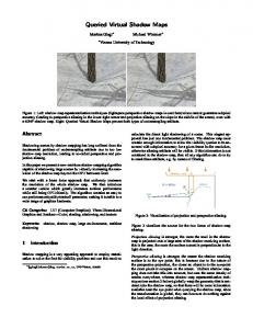
Figure 1: Left: Shadow map reparametrization techniques (lightspace perspective shadow maps is used here) alone cannot guarantee subpixel accuracy for neither all light directions nor large scenes, even with the largest shadow map supported by the GPU. Right: Fitted Virtual Shadow Maps allow the scene to be shadowed with subpixel accuracy.
A BSTRACT
otherwise aliasing artifacts will be visible. If this information is not contained in the shadow map, then all any algorithm can do is try to mask these artifacts, e.g. by means of filtering.
Too little shadow map resolution and resulting undersampling artifacts, perspective and projection aliasing, have long been a fundamental problem of shadowing scenes with shadow mapping.
Please see the introduction section in [8] for a definition of the two types of shadow map aliasing, projection and perspective aliasing.
We present a new smart, real-time shadow mapping algorithm that virtually increases the resolution of the shadow map beyond the GPU hardware limit where needed. We first sample the scene from the eye-point on the GPU to get the needed shadow map resolution in different parts of the scene. We then process the resulting data on the CPU and finally arrive at a hierarchical grid structure, which we traverse in kd-tree fashion, shadowing the scene with shadow map tiles where needed.
Aila et al [1] and Johnson et al [10] elegantly bypass the aliasing problem altogether but depend on hardware extensions for realtime performance which are not currently available. A straightforward way to increase the information contained in a uniform shadow map is to increase the resolution of the shadow map texture. This becomes impractical very fast, due to its quadratic increase in memory consumption (on current hardware the maximum supported texture size, typically 4096 × 4096 is the limiting factor, even before running out of memory).
Shadow quality can be traded for speed through an intuitive parameter, with a homogenous quality reduction in the whole scene, down to normal shadow mapping. This allows the algorithm to be used on a wide range of hardware.
This paper presents an algorithm which runs on current graphics hardware and increases the effective shadow map resolution available to shadow the scene, while avoiding the quadratic increase in memory consumption.
CR Categories: I.3.7 [Computer Graphics]: Three-Dimensional Graphics and Realism—Color, shading, shadowing, and texture Keywords: shadowing 1
From a practical point of view a common complaint that e.g. game developers have with the popular reparametrization techniques is that there is a large quality difference between the best and the worst case (as also shown by Lloyd et al [12]). The presented algorithm addresses this criticism and allows for the same shadow quality in all cases, while being orthogonal to shadow map reparametrization techniques and shadow map focusing. It can therefore be combined with these techniques, and we have done so for Light Space Perspective Shadow Maps [19] together with shadow map focusing [3].
shadow, shadow map, large environments, realtime
I NTRODUCTION
Shadow mapping is a very appealing approach to employ rasterization to solve the first hit visibility problem and use this result to calculate the direct light shadowing of a scene. This elegant approach has just one fundamental problem: The shadow map must contain enough information to allow the visibility queries to be answered with subpixel accuracy for a given frame buffer resolution,
1.1
Abbreviations
The following is a list of abbreviations used in this paper:
∗ {giegl|wimmer}@cg.tuwien.ac.at, 1040 Vienna, Austria
FVSMs: Fitted Virtual Shadow Maps, LiSPSM: Lightspace Perspective Shadow Maps [19], SM: Shadow Map, SMing: Shadow Mapping, SM-Tile: Shadow Map Tile (see section 3), SMTMM: Shadow Map Tile Mapping Map (see section 4).
1
To appear in a IEEE TCVG sponsored conference proceedings 2
P REVIOUS WORK
works as follows: 1. Allocate the biggest shadow map texture supported by the GPU. For example 40962 .
The two most important categories of shadow algorithms are shadow volumes [5] and shadow mapping [18].
2. Partition the shadow map along the shadow map x- and yaxis into n × n (e.g. 16 × 16) equally-sized SM-tiles (each tile using the full shadow map texture resolution of e.g. 40962 texels, i.e. the effective resolution of the full shadow map in this example is (16 ∗ 4096)2 = 655362 ).
Most of the shadow map publications try to solve the problem of aliasing artifacts. Percentage closer filtering [15] alleviates reprojection problems by sampling the shadow map. In Variance Shadow Maps, Donelly et al [6] use the variance of the depth values to further improve the shadow map sampling results. A number of papers have tried to solve the perspective aliasing coming from the perspective view frustum projection. Originally pioneered by Stamminger and Drettakis [16], who try to remove perspective aliasing by subjecting the shadow map to the same perspective transform as the viewer, this idea was later refined by Martin and Tan [13] with Trapezoidal Shadow Maps, Wimmer et al [19] with Light Space Perspective Shadow Maps and Chong et al [4] with A Lixel for Every Pixel. However, all shadow map reparametrization methods deal only with perspective aliasing. They cannot increase the principal resolution of shadow maps, which would be necessary for example to improve projection aliasing, or in cases where the scene is simply too large for the SM resolution. Furthermore, they work well only for the case that light and view direction are orthogonal. If these directions are parallel, they have to revert to uniform shadow mapping because the shadow map parametrization runs across the whole screen, not from near to distant points. Recently Lloyd et al [12] have studied the use of more than one shadow map applied to the sides or slices of the view frustum together with reparametrization techniques intensively, with interesting results; all these approaches can however only deal with perspective aliasing, but can do nothing to alleviate projection aliasing. The work presented in this paper aims to increase the resolution of shadow maps regardless of the view frustum orientation or whether the artifacts come from perspective or projection aliasing.
For each tile (a) Render a shadow map into the shadow map texture (overwriting the shadow map for the previous tile). (b) Use it immediately to shadow (modulate) the part of the scene which is covered by the current shadow map tile. There are two ways to implement the loop over the tiles: multi-pass shadowing and virtual deferred shadowing.
3.1
One way to apply successive shadow map tiles to the scene is by multi-pass rendering. In the first pass, the scene is rendered normally (with full shading and depth-writes enabled), with the first shadow-map tile applied to it. For each subsequent shadow-map tile, the scene is rendered again, but only shadow mapping using the relevant tile is applied to the frame buffer. Pixels falling outside the shadow map tile are suppressed. Depth writes and shading are disabled and the depth comparison function is set to EQUAL in those passes (depending on driver support, it can make sense to substitute LESSEQUAL for EQUAL).
Another approach to solve the aliasing problem are adaptive shadow maps [7] (see also section 4.8 below for a comparison with Fitted Virtual Shadow Maps), where shadow maps are stored in a hierarchical fashion in order to provide more resolution where it is required due to different aliasing artifacts. However, the approach requires multiple readbacks and does not map well to current graphics hardware. Lefohn [11] has proposed an extension that makes better use of the GPU, whereas Arvo [2] slices the light view to increase the resolution of the SM.
3.2
Deferred Shadowing
Multi-pass shadowing, although easy to implement, comes with a significant performance overhead of rendering the whole scene several times. To speed up the application of the shadow map tiles to the scene, we use a variation of deferred shading we call “deferred shadowing” where the shadowing is done using a linear depth buffer of the scene instead of re-rasterizing the scene geometry and the information needed to do the next shadowing pass, i.e., the next shadow map tile, is created on the fly between the passes. The scene is first rendered to a texture that stores eye-space depth, called the “Eye-Space Depth Buffer”. Each subsequent tiled shadowing pass can then read this texture and calculate the world-space position of the visible surface at each pixel using the screen coordinates and the depth stored in the Eye-Space Depth Buffer. The worldspace position is then shadowed using the shadow map tile as before. Note that storing the unmodified eye-space z-coordinate in the Eye-Space Depth Buffer guarantees that the shadow map lookup produces the same results as if the original scene objects were used for shadow mapping. This is important because any other method of obtaining the z-value, e.g., using window-space z-coordinates (which is highly non-linear) or a fixed-precision w-buffer (if it were still supported on current hardware) would inevitably lead to image artifacts. In detail this works as follows:
Second depth shadow mapping [17] can be used to reduce problems due to depth quantization and self occlusions. Brabec et al [3] improve uniform shadow map quality by focusing the shadow map to the intersection of the view frustum with the scene. Recently Queried Virtual Shadow Maps [8] have used the occlusion query mechanism of GPUs to adaptively refine the shadow map in quadtree fashion based on counting the number of pixels that changed in the shadow during the last refinement step. An excellent overview of shadow mapping and shadow algorithms in general can also be found in M¨oller and Haines’ Real-Time Rendering book [14], as well as in [9].
3
Multi-Pass Shadowing
V IRTUAL T ILED S HADOW M APPING
1. In a first pass, render the scene as described above, but into a 4 component 32bit floating point render target. In the pixel shader, store the unmodified eye-space z-coordinate into the α-component. This component forms the Eye-Space Depth Buffer (however for simplicity, we refer to the whole 4 component target as the Eye-Space Depth Buffer). The color of
The following section explaining Virtual Tiled Shadow Mapping, on which Fitted Virtual Shadow Mapping is based, is reproduced from [8]. Virtual Tiled Shadow Mapping is a brute-force approach for increasing the resolution of the shadow map beyond the maximum texture size supported by the hardware. The basic algorithm
2
To appear in a IEEE TCVG sponsored conference proceedings each pixel in the object when lit by this light (ignoring shadowing) is written to the RGB channels. 2. For each shadow-map tile (a) Render a shadow map into the shadow map texture as with Multi-Pass Shadow Mapping. (b) Instead of rendering the geometry for the whole scene again, render a full-screen quad with the Eye-Space Depth Buffer bound as a texture. (c) In the pixel shader for each fragment, look up the eyespace depth of the fragment in the Eye-Space Depth Buffer’s alpha-channel and unproject it into world space (see below). Using the unprojected fragment, calculate the shadowing term. Then modulate the already shaded RGB value from the Eye-Space Depth Buffer with the shadowing term. (d) The resulting shaded and possibly shadowed fragment is then written to the frame buffer.
Figure 3: Shadow Map Tile Mapping Map (SMTMM) creation.
The pixel shader operations in the individual passes are quite straightforward, with the exception of the unproject operation. Unlike a standard viewport unprojection, which transforms from window (xw , yw , zw )-coordinates to eyespace (xe , ye , ze )-coordinates, this operation has to deduce eye-space (xe , ye , ze ) from (xw , yw ) (given as texture coordinates, i.e. running from 0 to 1) and ze . This can be done using the following matrix transform:
1
xe ax ye = z e · 0 ze 0
0
− baxx
1 ay
− ayy 1
0
b
2 0 · 0
0 2 0
Map” (“SMTMM”; see Figure 3). The SMTMM contains information for each pixel in the scene about 1) where the pixel will query the shadow map, when inquiring whether it lies in the shadow, and 2) what resolution the shadow map would require along each SM-axis at this position to supply subpixel accuracy when answering the shadow map query. 3. Transfer the SMTMM to CPU memory and process it to create the “Shadow Map Tile Grid”. The Shadow Map Tile Grid contains information about what resolution each SM-tile of a virtual n × n Tiled SM would need along each SM-axis to supply subpixel accuracy when used to shadow the scene.
1 xw −1 · yw 1 1 (1)
4. Construct the “Shadow Map Tile Grid Pyramid” above the Shadow Map Tile Grid, by pulling up the maximum needed SM-tile resolution along each axis.
where the parameters ax , ay , bx , by in the first matrix should be taken from the projection matrix P supplied to the graphics API: ax 0 P= 0 0
4
0 ay 0 0
bx by ... 1
5. Traverse the Shadow Map Tile Grid Pyramid recursively top down, building an implicit kd-tree of SM-tiles. When the resolution requirement of a such created SM-tile can be satisfied along both SM-axes with a SM-tile-texture with dimensions supported by the GPU, the corresponding SM-tile shadow map is created and immediately used to shadow its part of the scene as under Deferred Shadowing (section 3.2) above.
0 0 ... 0
F ITTED V IRTUAL S HADOW M APPING
4.1
The following explains the steps in more detail and in section 4.10 introduces an important optimization to the basic algorithm:
Fitted Virtual Shadow Maps: Smart Refinement Where Necessary
4.2
Like Queried Virtual Shadow Maps, Fitted Virtual Shadow Maps aim to refine the shadow map only where needed. The algorithm is also designed to be fast enough to do the full refinement each frame. Instead of counting the number of changed shadow pixels in the last refinement step, and use this metric to decide whether to further refine a SM-tile into 4 sub-tiles, FVSMs try to discern beforehand what SM-resolution is needed where in the scene.
Virtual Shadow Mapping Preparation: Eye-Space Depth Buffer
First, we render the view-space depth information of the scene into the Eye-Space Depth Buffer, as above under 3.2. For efficiency reasons we again use a 4× f loat RGBA-buffer and at the same time render into it the unshadowed RGB color of the scene, so we do not have to rerender the scene (Note: If an application is using depthfirst rendering, i.e. starting with a Z-only pass, then a 1 × f loat buffer should be used for the Eye-Space Depth Buffer for the Zonly pass, with a conventional 1/z-depth buffer attached).
The following gives an overview over the FVSM algorithm (please see the following sections for details): 1. Render the view-space linear depth information of the scene into the Eye-Space Depth Buffer, as above under Virtual Tiled Shadow Mapping.
4.3
2. Use the Eye-Space Depth Buffer bound to a fragment-shader to create what we call the “Shadow Map Tile Mapping
The “Shadow Map Tile Mapping Map” (“SMTMM”) is a 4 × byte buffer. One can think of it as being laid on top of the frame
3
Shadow Map Tile Mapping Map Creation
To appear in a IEEE TCVG sponsored conference proceedings
(a) 40962 normal SM
(b) FVSM with 32 × 32 max SM-tiles
Figure 2: Quality comparison at end of test path through winter forest (LiSPSM SM reparametrization active in all screenshots).
buffer, normally having less resolution than the frame buffer, and containing information about the shadow map resolution needs of the scene in the area that each SMTMM “pixel” covers. Figure 3 gives a graphical representation of the SMTMM.
a byte value, we use the following formula: −log2 (round(∆sm axis + f loat2(0.5, 0.5))/256 (i.e. we output it as a logarithmic value normalized to the range [0, 1], which the the graphics hardware again automatically converts to byte range).
The first two byte values in each SMTMM entry (“pixel”) contain information about the position where the center of the frame buffer rectangle will query the shadow map; the last two byte entries represent the resolution needed along each SM-axis at the position in the shadow map. We use byte values for the entries, to keep the read back operation and the CPU processing in the next step fast; for the same reason, the SMTMM is normally chosen to have lower resolution than the frame buffer (see the results section for a practical range of values). Using byte values for the shadow map gives us information about the needed SM-resolution discretized to a 256 × 256 grid of SM-tiles; this is no restriction in practice, since one finds that for 40962 SM-tile-textures, a maximum refinement along each SM-axis of 16 to 32 (i.e. max 32 × 32 SM-tiles) gives subpixel accuracy even for large scenes.
The full SMTMM creation pixel shader can be found in Appendix A.
4.4
Shadow Map Tile Grid Creation
To create the “Shadow Map Tile Grid” (“SMTG”) we then read back the SMTMM to CPU memory. In practice it suffices for the SMTMM to have lower resolution than the frame buffer, e.g. 256 × 256, which makes the readback and CPU processing fast (note that the equality of the SMTMM dimension of 256 in this example and the number 256 of distinct values in the SMTMM entries is coincidental).
The position in the shadow map is calculated in the pixel shader by transforming the screen-space coordinates (xw , yw ) of the pixel (passed to the pixel shader as texture coordinates) and the eye-space z (=depth) entry ze , read from the Eye-Space Depth Buffer, into eyespace (xe , ye , ze ) using the matrix given in section 3.2 (formula (1)); from there it is transformed into the light space of the shadow map. Since the coordinates will already be in the range [0, 1], simply outputting them to the 4 × byte SMTMM surface will automatically lead to conversion into [0, 255] byte range by the graphics hardware.
What we want is a n × n SM-tile-grid structure, with each grid cell containing the needed resolution along each SM-axis and the screen space bounding rectangle for each SM-tile, an axis aligned rectangle around the pixels on screen that are affected by the SMtile. As in brute force n × n Virtual Tiled Shadow Mapping above, n is the maximum number of SM-slices along each SM-axis we would like to allow; a typical value for n would be 16 or 32, corresponding to 256 or 1024 SM tiles for Virtual Tiled Shadow Maps. The random memory access ability of the CPU is well suited for this task; after having read back the SMTMM, we lock the surface and process each pixel entry: We use the stored information about the SM-tile position to access its corresponding SM-tile-grid cell, and update 1) its needed SM-resolution entries along each SM-axis (minimally by maximizing the existing value with the entries in the SMTMM; see below for details) and 2) its screen space bounding rectangle (through extending it to enclose the pixel position of the current pixel in the SMTMM).
The resolution requirement along each SM-axis is approximated as follows in the pixel shader: First we calculate the (x, y)-coordinates of the neighboring pixels in x- and y-direction in [0, 1]2 (i.e. the left/right and upper/lower neighbors position in texture coordinates) from the texture coordinate of the current pixel passed to the pixelshader. We then use these texture coordinate to look up the corresponding view-space depth values in the Eye-Space Depth Buffer; from these, we calculate the smaller absolute ∆z along the x- and y-axis, ∆zx and ∆zy . We then use these ∆z values together with the x,y-coodinates of the neighboring pixels to construct an approximate rectangle representing the current pixel in space. Then we project this rectangle into SM-space, and calculate a SM-axisaligned bounding box around it. The half length of each of this bounding box’s extent, ∆sm axis , with sm axis = {0, 1}, is then used as the base measure for the required SM-resolution along each SMaxis at this point.
Since the SMTMM generally is chosen to have a much larger resolution than the SM-tile-grid, e.g. 256 entries per axis compared to e.g. 32, data from several SMTMM entries will be accumulated in the same SM-tile-grid cell. Minimally it would suffice to only record the maximum needed resolution along each SM-axis in each grid cell; however, to be able to allow for discarding very few pixels requiring a large resolution later on (which can come from e.g. a very small area on screen having an orientation which leads to large projection aliasing), we
To then quantize the needed SM-resolution along the SM-axis into
4
To appear in a IEEE TCVG sponsored conference proceedings actually count the number of pixels in each grid cell requiring a certain resolution. We use fixed size arrays at each SM-tile-grid-cell, to hold the pixel count statistics. To allow us to use fixed size arrays and keep them small, we count the number of pixels below a resolution η0 and above threshold resolution η1 in one array entry respectively, and the number of pixels needing a resolution in between each in their own entry; this is to keep cache locality high, since we are not interested in the detailed statistics of pixels with very small resolution requirements, because evidently they are easy to fulfill, and hypothetical pixels with extremely high resolution requirements, which do not occur in practice. See the results section for practical values for η0 and η1 .
smtgp(i_pyramid) = smtg for ix = 0 to smtgp(i_pyramid).n - 1 for iy = 0 to smtgp(i_pyramid).n - 1 SMTGP_Grid_Cell c_curr = smtgp(i)(ix,iy) SMTGP_Grid_Cell c_parent = smtgp(i-1)(ix >> 1,iy >> 1) // Update the screen-space, axis aligned bounding box // around the parent SM-tile c_parent.abb_screen.ExpandToIncludeABB(c_curr.abb_screen) // Update the maximum needed SM-resolution c_parent.sm_res_x = MAX(c_parent.sm_res_x,c_curr.sm_res_x) c_parent.sm_res_y = MAX(c_parent.sm_res_y,c_curr.sm_res_y) i_pyramid = i_pyramid >> 1
The following pseudocode illustrates the basic version of the Shadow Map Tile Grid Creation:
4.6
// smtg ... instance of the SMTG // shift ... shift-converts from the SMTMM SM-coordinates // entries to SMTG ones (e.g. [0,255] => [0,31]) const int shift = 256/smtg.n // smtmm ... instance of the SMTMM // smtmm.n ... extent of SMTMM along both axes for ix_smtmm = 0 to smtmm.n - 1 for iy_smtmm = 0 to smtmm.n - 1 SMTMM_Cell c_smtmm = smtmm(ix_smtmm,iy_smtmm) SMTG_Cell c_smtg = smtg(smtmm.ix_sm >> shift,smtmm.iy_sm >> shift) // Update the screen-space, axis aligned bounding box // around the SM-tile c_smtg.abb_screen.ExpandToIncludePoint( ix_smtmm/smtmm.n,iy_smtmm/smtmm.n ) // Update the maximum needed SM-resolution c_smtg.sm_res_x = MAX(c_smtg.sm_res_x,c_smtmm.sm_res_x) c_smtg.sm_res_y = MAX(c_smtg.sm_res_y,c_smtmm.sm_res_y)
4.5
Shadow Map Tile Grid Pyramid Traversal
Finally we traverse the grid pyramid top down, building an implicit kd-tree as we recursively traverse it, as follows: If the resolution requirement of the SM-tile-grid cell along at least one axis cannot be satisfied with a SM-tile-texture with dimensions supported by the GPU (e.g. on current GPUs typically: required SM-dimension > 4096), we split it symmetrically along one or both SM-axis into 2 or 4 subcells. We split into 2 subcells if only one axis has SM resolution requirements which cannot be fulfilled, otherwise we split into 4 subcells. Otherwise we use Deferred Shadowing (see section 3.2), and immediately create the SM-tile with the required resolution along each axis and shadow the “Shadow Result Texture” (see next paragraph) with it, using the Eye-Space Depth Buffer to get the depth values of the scene, as described in section 3.2. The “Shadow Result Texture” is a 1 × byte texture with the same dimensions as the frame buffer, into which we write only the results of the shadowing. This makes the application of the SM-tiles faster, since we write to a surface with only one byte entry per pixel; it also allows us to avoid any potential problems with slightly overlapping SM-tiles, since shadowing results of a tile which is applied later can simply overwrite previous results. (The Shadow Result Texture can also be used to apply postprocessing effects to the shadow, such as screen space blurring depending on distance to the shadow caster.)
Shadow Map Tile Grid Pyramid Creation
After we have filled the SM-tile-grid with data from the SMTMM, we proceed by building a pyramid (“Shadow Map Tile Grid Pyramid”, “SMTGP”) of SM-tile grids on top of it, where each successive grid has halved dimensions of its predecessor and the needed resolution along each SM-axis is the maximum of the corresponding 2 × 2 grid cells in the predecessor grid; i.e. we pull up the needed resolution along each SM-axis by replacing 2 × 2 cells with one cell in the next smaller grid, containing the maximum value of each of the 4 cells and the screen space bounding rectangle around all 4 bounding rectangles.
Pseudocode for the traversal of the Shadow Map Tile Grid Pyramid: // SMT ... SM-tile instance // P ... SMTGP pos index + pyramid index // smtq ... queue holding SMT smtq.push(SMT(P(0,0),P(0,0))) while(!smtq.empty()) SMT smt = smtq.pop() int ip_x = smt.ip_x, int ip_y = smt.ip_y int sx = max(0,ip_y-ip_x), int sy = max(0,ip_x-ip_y) Rect rect(ix