Hybrid Finite Element and Volume Integral

c 2000 Tech Science Press Copyright

CMES, vol.1, no.1, pp.11-24, 2000

Hybrid Finite Element and Volume Integral Methods for Scattering Using Parametric Geometry John L. Volakis1 , Kubilay Sertel1 , Erik Jørgensen2 , and Rick W. Kindt1

Abstract: In this paper we address several topics relating to the development and implementation of volume integral and hybrid finite element methods for electromagnetic modeling. Comparisons with the finite elementboundary integral method are given in terms of accuracy and computing resources. We also discuss preconditioning, parallelization of the multilevel fast multipole method and propose higher-order basis for curvilinear quadrilaterals and volumetric basis functions for curvilinear hexahedra. The latter have the desirable property of vanishing divergence within the element but non-zero curl. In addition, a new domain decomposition is introduced for solving array problems involving involving several million degrees of freedom. Three orders of magnitude CPU reduction is demonstrated for such applications.

this paper we review some recent progress in modeling volumetric scatterers with particular emphasis on materials having non-trivial permeability.

Initial efforts in modeling dielectric scatterers date back to the 1960s with J. H. Richmond, (1965) (see also A. F. Peterson, (1998) for a partial review of volume formulations) being among the first who published a numerical solution for the scattering by purely dielectric cylinders. Extensions to three dimensional scattering were carried out later by D. E. Livesay and K. Chen, (1974), D. H. Schaubert, D. R. Wilton, and A. W. Glisson, (1984), and R. D. Graglia, P. L. E. Uslenghi, and R. S. Zich, (1989). These solutions brought about the realization that practical size simulations of such targets were not possible using traditional integral equation solvers due to excessive O(N 2 ) and O(N 3 ) memory and CPU requirements, respectively. Thus, so far, applicakeyword: Radar scattering, magnetic materials, vol- tions of volume integral integral equations have been limume integral equations, finite-element boundary-integral ited to small and mostly purely dielectric structures. method, fast multipole method, parallelization, antenna radiation, preconditioning, curvilinear elements, higher- During the 1990s, treatment of inhomogeneous scatterers focused on finite element (FE) methods and their hyorder basis functions. brid finite element-boundary integral (FE-BI) counterparts [J. L. Volakis, T. Ozdemir, and J. Gong, (1997); 1 Introduction J.L.Volakis, A. Chatterjee and L. Kempel, (1998)]. These Electromagnetic scattering by inhomogeneous structures were found attractive because of their geometrical and is of great interest in evaluating the overall scattering by material adaptability coupled with their lower memory modern composite vehicles. The same mathematical for- requirements. The introduction of fast integral methmulations are also suited for antennas, high frequency ods [W. C. Chew, J.-M. Jin, E. Michielssen, and J. Song, microwave circuits, electromagnetic coupling and inter- ed., (2001)] prompted renewed interest in the solution of ference, and inverse scattering applications. Thus, much volume integral equations (VIEs) [J. L. Volakis, (1992)] interest exists in developing efficient formulations and for practical problem simulations. This interest is also numerical solutions in modeling volumetric scatterers motivated by the inherently fast convergence of VIE mahaving arbitrary permittivity (ε) and permeability (µ). In trix systems as compared to corresponding systems generated via the FE-BI. 1 Department

of Electrical Engineering and Computer Science, Radiation Laboratory, University of Michigan, 48109, Ann Arbor, MI. 2 Erik Jørgensen was at the Univ. of Michigan. He is now at the Technical University of Denmark, Ørsted–DTU Electromagnetic Systems, Ørsteds Plads, DK–2800 Lyngby, DENMARK.

In this paper we consider volume integral and hybrid FE-BI formulations for scattering by inhomogeneous structures. In addition to the comparison of these formulations, several other unique features are covered

12


CMES, vol.1, no.1, pp.11-24, 2000

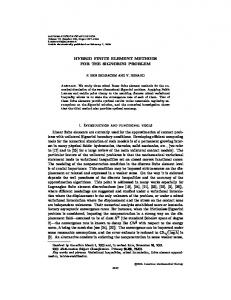
in the paper. Specifically, we introduce three dimenε0 , µ0 inc sional curvilinear elements for discretizing VIEs assoE (r) ciated with inhomogeneous structures (essential for acr z ε(r) , µ(r) curate modeling of high contrast dielectrics [J.-M. Jin, J. L. Volakis, and V. V. Liepa, (1989)]), multilevel fast r´ v multipole method (MLFMM) implementation of the ass y sociated systems, and related parallelization issues. Also, x new hierarchical basis for improved convergence of the iterative solvers are introduced along with precondition- Figure 1 : Geometrical setup for VIE and FE-BI formuing techniques. Throughout the paper, emphasis is on the lations treatment of permeable dielectrics, and solutions are presented (for the first time) for three dimensional structures with non-trivial permeability. Furthermore, all implementations were focused on nonmagnetic volumes. However, for practical modeling of 2 Volume Integral Equation Formulation man-made structures, there is a requirement to allow for To derive a general integral equation for inhomoge- the presence of non-trivial permeability. Next, we introneous structures, we start with the VIE for an inhomo- duce an integral equation which avoids surface integrals. geneous dielectric structure in a source-free region given To this end, we note that the dual of Eq. (1) is by [R. F. Harrington, (1968)]

inc

E(r) = E

(r)+k02

Z

v

dv0 G(r, r0 )·(εr (r0 )−1)E(r0 ). (1)

Einc

H(r) = Hinc (r) + k02

Z

v

dv0 G(r, r0 ) · (µr (r0 ) − 1)H(r0 )

(4)

In this, is the incident electric field or excitation, E is the total field within the domain (see Fig. 1), k0 = √ ω ε0 µ0 = 2π/λ0 is the free-space wavenumber, εr (r) and since ∇ × E(r) = iωµH(r), it follows that the comis the relative dielectric constant of the inhomogeneous plete integral equation for general volumes is medium, and Z inc 2 E(r) = E (r) + k dv0 G(r, r0 ) · (εr (r0 ) − 1)E(r0 ) 1 0 0 0 v G(r, r ) = I + 2 ∇∇ g(r, r ) (2) Z k0 + dv0 ∇0 × G(r, r0 ) · (µr (r0 ) − 1)∇0 × E(r0 ).(5) v is the free-space dyadic Green’s function with 0

eik0 |r−r | g(r, r ) = |r − r0 |

(3) We note here that in contrast to the volume-surface integral equation given earlier [J. L. Volakis, (1992)], this representation does not involve any surface integrals. (an e−iωt time convention is assumed and suppressed). This integral equation is implemented below and valiNumerical solution of this VIE has been given by sev- dated for the first time using curvilinear elements. Beeral authors using various forms. D. E. Livesay and low, we proceed to discretize the VIE for any basis exK. Chen, (1974) were the first to solve Eq. (1) us- pansion. The specific curvilinear representation is given ing brick elements with piecewise constant expansions. in the Appendix. Later D. H. Schaubert, D. R. Wilton, and A. W. Glisson, As usual, to discretize Eq. (5), we introduce the expan(1984) employed tetrahedra with linear basis functions, sion and R. D. Graglia, P. L. E. Uslenghi, and R. S. Zich, N (1989) considered a moment method implementation of E(r) ≈ ∑ ai ei (r). (6) dielectric volumes using isoparametric elements. i=1 0

So far, simulations have been limited to small problems due to excessive memory and CPU requirements. Substituting this into Eq. (5), and employing Galerkin’s

13

Hybrid Finite Element and Volume Integral Methods

testing gives the matrix system Za = b, where Z ji

Appendix), the divergence is more easily computed using covariant representations, whereas the curl is more = he j (r), ei (r)i easily computed using contravariant ones [A. F. Peterson Z and D. R. Wilton, (1996)]. Thus, care must be employed − he j (r), k02 dv0 G(r, r0 ) · (εr (r0 ) − 1)ei (r0 )i in whether a covariant or a contravariant form should be Z v used. One approach is to employ a mix of these represen0 0 0 − he j (r), dv ∇ × G(r, r ) tations as is best suited for the evaluation of the various v 0 0 0 · (µr (r ) − 1)∇ × ei (r )i (7) integrals.

and b j = he j (r), Einc (r)i.

(8)

3 Finite Element-Boundary Integral Equation Formulation The inner-product integrals over the source and testing domains appearing in Eq. (7) require a series of algebraic manipulations before they can be accurately imple- Finite element (FE) [J. L. Volakis, T. Ozdemir, and mented in a numerical solution. Specifically, for self-cell J. Gong, (1997); J.L.Volakis, A. Chatterjee and L. Keminteractions careful numerical quadrature evaluation is pel, (1998); J. L. Volakis, T. F. Eibert, and K. Sernecessary due to the singular nature of the Green’s dyadic tel, (2000)] and finite element-boundary integral (FE-BI) and its curl [K. Sertel and J. L. Volakis, (2002)]. For the methods have been among the workhorse techniques for frequency domain simulations over the past ten years. first integral in Eq. (7), namely, Here, we present a brief overview for comparison with Z the VIE given above. The FE-BI is also presented 2 0 0 0 0 I1 = he j (r), k0 dv G(r, r ) · (εr (r ) − 1)ei (r )i from a general viewpoint as applied to non-planar strucv Z 1 tures [G. E. Antilla and N. G. Alexopoulos, (1994)] and = he j (r), k02 dv0 (I + 2 ∇∇g(r, r0 )) is further optimized for large finite arrays. k0 v ·

(εr (r0 ) − 1)ei (r0 )i

(9) In formulating the FEM, we begin with the functional

it is necessary and customary to transfer one of the derivatives on the scalar Green’s function to the testing function. This is accomplished through the divergence theorem as given in the Appendix of K. Sertel and J. L. Volakis, (2002). Evidently, for basis/testing functions having discontinuous normal components over adjacent elements, it is also necessary to evaluate the surface integral over element faces, appearing after the application of the divergence theorem [K. Sertel and J. L. Volakis, (2002)]. However, if the basis/testing functions are chosen to satisfy normal continuity, these surface integrals vanish (as discussed in D. H. Schaubert, D. R. Wilton, and A. W. Glisson, (1984)). The resulting integrals can be evaluated using the annihilation method (for general curvilinear coordinates), which converts first-order singular integrals into non-singular integrals for numerical integration as given in K. Sertel and J. L. Volakis, (2002).

F(E) =

1 2

Z

dv

v

− ik0 Z0

Z

s

1 (∇ × E) · (∇ × E) − k02 εr E · E µr

ds(E × H) · nˆ

(10)

where the boundary integral S encloses the volume V (see Fig. 1). It is necessary to relate E and H on the surface to obtain a single functional in terms of E only. This is done by introducing the Stratton-Chu integral equation [A. J. Poggio, (1973)]. The electric field integral equation (EFIE) version of this is Θ(J) − Ω(M) = Einc ,

(11)

whereas the magnetic field integral equation (MFIE) has We remark that the curl and divergence operations on the the form testing and basis functions implies use of at least linear expansion functions. For curvilinear brick elements (see Ω(J) + Θ(M) = Hinc , (12)

14


CMES, vol.1, no.1, pp.11-24, 2000

in which Θ(X) = −ik0

Z

ds0 G(r, r0 ) · X(r0 )

= −ik0

Z

ds0 g(r, r0 )X(r0 )

+

i k0

Z

s

s s

ds0 ∇g(r, r0 )∇0 · X(r0 )

(13)

Z

Ω(X) = T Y(r) + −ds0 X(r0 ) × ∇g(r, r0 ) s

with Y = −nˆ × X, T = 1 − β/4π, and nˆ denoting the unit normal to the bounding surface (β = 2π for a smooth surface). Typically, a linear combination of the two, referred to as the combined field integral equation (CFIE) is employed to avoid resonance difficulties and poor conditioning.

time, especially for multi-spectral simulations. Preconditioning methods may therefore be necessary for certain problems to achieve convergence (see R. D. Graglia, P. L. E. Uslenghi, and R. S. Zich, (1989); J.-M. Jin, J. L. Volakis, and V. V. Liepa, (1989); G. E. Antilla and N. G. Alexopoulos, (1994) and for higher-order basis functions see R. D. Graglia, D. R. Wilton, and A. F. Peterson, (1997); B. M. Kolundzija and B. Popovic, (1993); J. P. Webb, (1999)). Clearly, it is important to use preconditioners which can be implemented in favorable CPU times. Among them, the ILU [K. Sertel and J. L. Volakis, (2000)] and block-diagonal [Y. Saad, (1996)] preconditioners have been found quite effective. In modeling layered geometries, substantial improvement in matrix condition can be achieved by choosing hexahedral elements rather than the usual tetrahedra. Curvilinear elements also allow for geometrical modeling fidelity and have been shown to be very effective for antenna arrays [R. W. Kindt, K. Sertel, E. Topsakal, and J. L. Volakis, (2003)] as well as scattering applications [R. D. Graglia, P. L. E. Uslenghi, and R. S. Zich, (1989)].

The electric field is solved from Eq. (10) by setting ∂F(E)/∂E = 0 and on discretizing the resulting equations using the appropriate expansion [G. E. Antilla and N. G. Alexopoulos, (1994)] results in the system      Evv Evs 0 Ev 0  Esv Ess B   Es  =  0  (14) When dealing with arrays, certain advantages associated 0 P Q Hs b with the repeatability of each array element can be exwhere the element matrices are given by ploited. More specifically, we observe from Fig. 2 that Z each element has identical geometry and thus the FE-BI Pji = −α dst j · Ω(ei ) matrix system takes the form s

+ (1 − α) Q ji = α bj = α

Z

Zs s

Z

s

dsnˆ × t j · Θ(ei )

dst j · Θ(ei ) + (1 − α) dst j · E

inc

+ (1 − α)

Z

Z s s

dsnˆ × t j · Ω(ei ) inc

dsnˆ × t j · H

(15)

with ei and t j being the expansion and testing functions for the surface quantities, respectively, and α is a scale factor chosen from zero to unity.

    

a11 a21 .. .

a12 a22 .. .

... ... .. .

a1M a2M .. .

aM1

aM2

...

aMM

   x1   x2   ..  .    xM

    

 b1     b2 = .     ..     bM

        

(16) where the sub-matrices a denote the individual coupling operators between the m and m0 elements in the array, {x1 , . . . , xM }T is a block-vector containing the unknown vectors for each array element, and {b1 , . . . , bM }T is also a block-vector providing the excitations on the array elements. Each of the diagonal submatrices is of the same form as given in Eq. (14), whereas the off-diagonal submatrices matrices describe the coupling among the m and m0 array elements (see Fig. 2). If we use a boundary integral to enclose the volume of each array element, then all off-diagonal submatrices will just contain the P and Q submatrices in Eq. (14). mm0

For a general, inhomogeneous structure consisting of material and conducting components, the resulting system in Eq. (14) is highly heteregeneous, consisting of a sparse FE part (E and B submatrices in Eq. (14)) and a full integral equation part (P and Q submatrices in Eq. (14)). In practice, this highly heteregeneous FE-BI system may result in a poorly convergent iterative solution, especially for large scale simulations. Since the application of fast methods (such as the MLFMM) implies use of iterative solvers, this poor convergence be- Of importance is that the coupling submatrices only havior introduces a bottleneck in terms of total solution depend on the absolute distance among elements and

15


[a] [a]

[a]

[a]

and thus the same clustering can be used for the surface electric field unknowns, leading to significant memory savings. A detailed discussion on the FFT acceleration for antenna arrays and the MLFMM implementation for the VIE and FE-BI systems is beyond the scope of this paper. However, several performance analyses and results are provided in the subsequent sections. 4

Figure 2 : Illustration of redundant coupling paths in a 1 × 6 array.

the diagonal submatrices are identical. Consequently, the overall matrix in Eq. (16) is block Toeplitz. Thus, Eq. (16) can be cast in the circulant form Π ∗ {x} = {b} where “∗” implies convolution and Π = {aM−1 . . . a1 /, a0 /, a−1 . . . a1−M } in which the notation amm0 = am−m0 = a p has been introduced. This observation implies that the fast Fourier transform (FFT) can be employed to carry out the matrix-vector products of the entire FE-BI system in O(N log N) CPU time and using O(N) storage.

Higher-order Basis Functions

As mentioned above, some key issues related to the efficient and accurate modeling of large scale structures are the discretization accuracy, error propagation and convergence of the iterative algorithms. Use of curvilinear elements allow for body conforming modeling. Thus, much fewer elements need be used to achieve the same accuracy. Fewer discretization elements also imply improvement in the condition number, leading to improved convergence. This is demonstrated in Tab. 1 which refers to a PEC sphere (the MLFMM was used to carry out the solution using linear conformal basis functions on quadrilateral surface patches). As can be observed, the same problem at the same frequency can be solved using 3.5 samples per λ in 10.1 s. per iteration vs. 38.4 s. per iteration if 10 samples per λ is used to still maintain acceptable error.

In addition to the above, we may further exploit the fact that all diagonal submatrices, i.e. amm0 = am−m0 = a p Table 1 : Convergence rates with different mesh densifor p = 0, are identical, and use the inverse of a0 to ties. precondition the entire matrix system. This type of Discretization Number of Time per Solution preconditioning has been found very effective once the Iterations Iteration(s.) time(s.) overall FE-BI matrix is re-structured as suggested in 3.5/λ 21 10.1 212.3 Eq. (16). Details of this decomposition method can 10/λ – 38.4 – be found in R. W. Kindt, K. Sertel, E. Topsakal, and J. L. Volakis, (2003). In closing this section, we note that the MLFMM can be readily incorporated into the FE-BI method to speed-up the solve time associated with large scattering and/or radiation problems having arbitrary shape. The MLFMM (already used for perfectly conducting targets) can be extended to both VIE and FE-BI methods by merely incorporating the signature functions into their respective algorithms. Specifically, for the FE-BI method, since the same basis functions are used for both surface unknowns (Es and Hs ), the same signature functions can be utilized for both. Also, the clustering of the surface unknowns is based solely on the surface magnetic field

A natural need in using larger elements is the employment of higher-order bases. Such bases have been extensively examined [R. D. Graglia, D. R. Wilton, and A. F. Peterson, (1997); B. M. Kolundzija and B. Popovic, (1993); J. P. Webb, (1999); L. S. Andersen and J. L. Volakis, (1999)] and can be categorized as either interpolatory or hierarchical. The latter are more attractive since they allow for using different order expansions at each element (surface or volume) of the discretized body. However, such higher-order bases may often lead to substantial deterioration in convergence. To improve convergence, we must improve the orthogonality of these


16

CMES, vol.1, no.1, pp.11-24, 2000

elements while still maintaining their hierarchality. Be- be matched with corresponding functions on the neighboring patches to enforce continuity of the normal curlow, we introduce such an expansion. Without loss of generality, let us consider the quadri- rent component. lateral patch defined in the local curvilinear (u, v) coordinate system, where 0 ≤ u, v ≤ 1. The patch can be bilinear, biquadratic, or even higher-order as determined by the position vector r(u, v) defining the patch surface. The surface current on the patch is expanded as Js = Jsu au + Jsv av , where au and av are the covariant ∂r unitary vectors au = ∂u and av = ∂r ∂v . Instead of the hierarchical expansion (only the u-directed currents are considered) introduced by B. M. Kolundzija and B. Popovic, (1993) Jsu = + +

+

1 N ∑ {c0n (1 − (2u − 1)) A n=0 c1n (1 + (2u − 1))} (2v − 1)n  N  M 1 ∑  m=2 ∑ cmn ((2u − 1)m − 1) A n=0 m even   M cmn ((2u − 1)m − (2u − 1)) ∑  m=3

(17)

m odd

where cmn are the constants of the expansion and A = |au × av |, we propose the alternative expansion [E. Jorgensen, J. L. Volakis, P. Meincke, and O. Breinbjerg, (2002)] (also polynomial) r 1 3 N Jsu = ∑ [b0n (1 − (2u − 1)) A 8 n=0 +

b1n (1 + (2u − 1))]Cnv Pn (2v − 1)

+

1 M N ∑ ∑ bmnCmu [Pm (2u − 1) A m=2 n=0

−

Pm−2 (2u − 1)]Cnv Pn (2v − 1)

(18)

where Pn (v) are the Legendre polynomials given by dn 2 n and b Pn (v) = 2n1n! dv n (v − 1) mn are the new expanq sion coefficients. The constants C um = (2m−3)(2m+1) 2(2m−1) √ and C vn = 2n + 1 are scaling factors chosen such that the Euclidian norm of each basis function is unity on a unit square patch. It is important to note that the polynomials 1 − (2u − 1), 1 + (2u − 1), P2 (2u − 1) − P0 (2u − 1), ..., PM (2u − 1) − PM−2 (2u − 1), can be shown to span the space of polynomials of degree M. Also, since the first two terms are non-zero at u = 0 or u = 1, they must

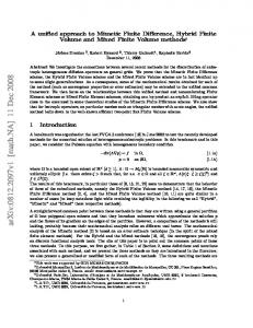
Although similar to the expansion in Eq. (17), the basis in Eq. (18) differs in three important ways. First, orthogonal polynomials are used. Second, the continuity equation is incorporated by modifying the polynomials in a way that preserves orthogonality as much as possible, and third, a scaling factor is included to improve the condition number. The interpolatory bases of R. D. Graglia, D. R. Wilton, and A. F. Peterson, (1997) are limited to a fixed approximation order corresponding to the choice N = M − 1. In this special case, all three bases (those in R. D. Graglia, D. R. Wilton, and A. F. Peterson, (1997); B. M. Kolundzija and B. Popovic, (1993) and Eq. (18)) span the same polynomial space, have the same number of unknowns in a single patch, and have the same number of unknowns associated with two patches. Consequently, the current obtained via the moment method will be identical for all three bases, although the implementation and condition number of the resulting matrix may differ significantly. To demonstrate the improved condition number of the new basis defined in Eq. (18), let us consider the scattering by a pair of parallel PEC plates solved via the EFIE. Fig. 3 shows the matrix condition number obtained with the bases in [R. D. Graglia, D. R. Wilton, and A. F. Peterson, (1997); B. M. Kolundzija and B. Popovic, (1993)] and those in Eq. (18). As seen (the annihilation technique in K. Sertel and J. L. Volakis, (2002) was used for the self-cells), the condition number appears to be exponentially increasing as the order of the hierarchical bases in B. M. Kolundzija and B. Popovic, (1993) increase, but remains fairly constant for our proposed hierarchical bases given by Eq. (18). This is important since large physical elements can be used with higher-order expansion without adverse effects on the system convergence.

5 MLFMM on Parallel Architectures The most CPU intensive component in any iterative solution of a dense matrix system is the execution of the matrix-vector product Za mentioned earlier. This is usually an O(N 2 ) operation which can be reduced to O(N log N) via the MLFMM procedure [W. C. Chew, J.M. Jin, E. Michielssen, and J. Song, ed., (2001); R. Coifman, V. Rokhlin, and S. Wandzura, (1993)]. Thus, the

17


Condition number

separate processors independently, without interprocessor communication. The only required communication will take place at the translation step when the source and target clusters lie on different processors. However, this requires a significant amount of communication between processors, as will be explained below. With vector pro2 3 4 5 6 cessing capabilities on computing platforms, the actual Polynomial degree work at the translation step on each processor is quite (a) (b) small and comparable to the time used for communicaFigure 3 : Condition number of the EFIE implemented tion. Consequently, communication among processors using different higher-order basis functions (Interpolabecomes a bottleneck for the parallel performance of the tory [R. D. Graglia, D. R. Wilton, and A. F. Peterson, MLFMM implementation. (1997)] and hierarchical power basis [B. M. Kolundzija and B. Popovic, (1993)]). 1.0e10 1.0e9 1.0e8 1.0e7 1.0e6 1.0e5 1.0e4 1.0e3 1.0e2

Interpolatory basis Hier. power basis This paper

1

MLFMM plays a most important role in the solution algorithm, and its parallelization is essential in porting the FE-BI or VIE solvers to distributed computing platforms. In considering the parallelization of the matrix-vector products in the MLFMM algorithm, we must examine the three basic steps within the algorithm: (1) the radiation, or signature functions of each group at the (n + 1)th level aggregated to form the radiation functions of the parent groups, i.e. groups at the (n)th level; (2) the translation of the radiation functions to cluster centers located in the far-zone of the source cluster at the (n)th level, provided their parents at the (n − 1)th level are in the nearzone of each other; (3) the disaggregation step, where the children clusters at the (n + 1)th level are disaggregated to compute the fields within the clusters. These three steps are depicted in Fig. 4 for a three-level FMM tree. A successful parallel implementation of these three steps requires • Careful balancing of the computational load among the processors, and • Minimal communication between the processors. Load balancing requires the distribution of the MLFMM tree structure on the nodes of the parallel process. For the sake of simplicity, let us consider the tree structure given in Fig. 4, consisting of 2 main clusters at the coarsest level. If the tree is distributed on 2 nodes of a parallel process, assuming that each cluster at each level has the same number of far-zone clusters, we would achieve a perfectly balanced distribution. For such a case, the aggregation and disaggregation steps can be carried out on

2

3

5

4

6

7

9 10 11 12

8

1

2

3

4

5

6

7

9 10 11 12

8

level 3

2

1

3

4

2

1

3

4

level 2 aggregations

disaggregations

1

1

2

level 1

2

sparse translations Proc. 1

down-tree pass

Proc. 2

Proc. 2

Proc. 1

up-tree pass

Figure 4 : A hypothetical MLFMM clustering tree.

To better explain the situation, let us assume that at the 1st level, clusters 1 and 2 are in the near-zone of each other. Furthermore, let us assume that at the 2nd level, clusters 1 and 2 are in the near-zone of each other (similarly, clusters 2 and 3 and clusters 3 and 4 are in the near-zone of each other) and clusters 3 and 4 lie in the far-zone of cluster 1 and clusters 1 and 2 lie in the farzone of cluster 4. Likewise, at the 3rd level, clusters 1 to 3 lie in the near-zone of each other and clusters 4 to 12 lie in the far-zone of clusters 1 to 3, and so on. Each processor can independently compute the aggregations at all levels starting from level 3 (we’ll call this the down-tree pass). Likewise, once the pertinent data is available, the disaggregations at all levels can be computed on separate processors, independently (up-tree pass). However, interprocessor communication is necessary for the translation operations since, for example, clusters 1 and 3 (at level 2) lie on different processors and the translation operation

c 2000 Tech Science Press Copyright Problem: 28812 Unknown Sphere

Problem: 28812 Unknown Sphere

16

16 Ideal Fill Time Solve Time

14

Ideal Fill Time Solve Time

14

12

12 Speed−up Factor

requires the radiation function of cluster 1 to be translated onto cluster 3. For level 2, the required number of operations for the translation step is 3 × 2L22 per processor. Thus the length of data that must be communicated between processors is 3 × 2L22 in each direction. For level 3 the situation is slightly different. If we had assumed that clusters 2 and 3 at level 2 were in the near-field of each other, we would need to execute 2 × 3 × 3 × 2L32 operations to evaluate the translated fields between the children of cluster 2 and 3 (at level 2). This simple example demonstrates the high rate of inter-processor communication needed at the translation step of the MLFMM algorithm. Via aggressive optimization in compiling the MLFMM code on computers with vector processing capabilities, the intra-processor work load can be significantly reduced. Hence, the inter-processor communication speed remains a bottleneck for optimal performance of the MLFMM on distributed memory parallel computers. Below, we present some preliminary performance data and point out the effects of inter-processor communication speed.

CMES, vol.1, no.1, pp.11-24, 2000

Speed−up Factor

18

10 8 6 4

10 8 6 4

2

2 2

4

8 Number of Processors

16

2

4

8 Number of Processors

16

(a) (b) Figure 5 : Performance of parallel MLFMM for a 28,812 unknown sphere, (a) no compiler optimizations, (b) –O4 compiler optimizations

the solution time was 8.2 times faster after compiler optimizations. In light of the above observations, we conclude that even for a very well balanced problem, interprocessor communication remains the bottleneck for the parallel performance of MLFMM on distributed memory computers. Consequently, future efforts must focus on As an example, consider the scattering by a sphere of significant re-organization of the MLFMM algorithm for 1m. radius. A balanced MLFMM grouping leads to 5 massively distributed platforms. MLFMM levels each with 8, 56, 272, 1157, and 4517 non-empty cubes. For parallelization, this tree is dis- 6 Comparison Data Between VIE and FE-BI Formulation tributed among processors on the basis of second level clusters, and the performance test was carried out on To validate the proposed VIE for magnetic materian IBM SP3 computer having three nodes, each with als, we consider a comparison of the scattering by a eight, 375 MHz Power3 processors (3 × 8 = 24 processphere (canonical problem) and a cube. A secondary goal sors). The high-speed switch connecting the three nodes is to provide an initial comparison of the solution perforcan deliver 500 MB/s bi-directionally to each processor. mance for the VIE and FE-BI methods for these specific Both the matrix-fill and the iterative solution time were structures. recorded to evaluate performance. Parallelization of the near-field matrix is straightforward and will not be dis- The considered sphere example refers to a purely dielectric problem. The sphere radius is 0.2λ and εr = cussed here. 2.592. As depicted in Fig. 6, the bistatic radar cross secSpecifically, we show the parallel performance for a 1 tion (RCS) patterns calculated using the FE-BI and VIE m radius sphere at 0.75 GHz. This problem resulted in methods are in excellent agreement with the exact Mie 28, 812 unknowns and as seen in Fig. 5, severe perforseries data. However, the FE-BI required more unknowns mance deterioration is observed due to inter-processor to achieve the same accuracy. Thus, to better compare communication. For the non-optimized code, better parthe VIE and FE-BI methods, we consider a comparison allelization performance is observed since the evaluation of the solution error vs. the element’s edge length (in of the translations has a significant computational burden both cases the same curvilinear hexahedra were used). at this step. However, for the optimized code (–O4 opThis comparison was done for the sphere example and retion), the inter-processor communication dominates after sulted in the curves given in Fig. 7. These depict that the the 4th processor is added, leading to saturation. We note error is proportional to the square of the element’s edge here that, for a serial run (single processor), the matrix length for both methods. However, the VIE √ can effort fill time demonstrated a speed-up factor of 3.7, whereas larger elements for the same error (∆V IE ≈ 2∆FE−BI ).

19


0

0

−5

−5

−10

−10

−15

−15

Bistatic RCS (dB)

−20

−25

−25

−30

Mie VIE (N = 300) VIE (N = 882)

−35

0

20

40

60 80 100 120 Observation Angle θ (Degrees.)

140

160

Mie FE−BI (N = 492) FE−BI (N = 1314)

−35

180

−40

0

20

40

60 80 100 120 Observation Angle θ (Degrees.)

140

160

180

(a) (b) Figure 6 : Bistatic RCS of a dielectric sphere of radius 0.2λ (εr = 2.592). (a) VIE Solution, (b) FE-BI Solution

0

−10

−20

−5

−30 −10 Bistatic RCS (dB)

−30

−40

−20

Bistatic RCS (dB)

Bistatic RCS (dB)

Also, as shown in Tab. 2, the VIE system converges much Table 2 : Performances of VIE and FE-BI formulations faster but the matrix fill is significantly higher for the VIE for the sphere. Number Matrix Number Time per formulation. The latter is a clear disadvantage of the VIE of Fill of per method, but the rapid convergence of its associated maUnknowns Time Iterations Solution trix system provides incentives for further examination (s.) (s.) of the method. Clearly, this comparison refers to a speVIE 300 107 11 0.41 cific example and should not be generalized at this stage. VIE 882 1211 13 5.00 Most likely, the FE-BI method will be a choice method 492 1.3 160 4.08 for many composite structures but the VIE offers advan- FE-BI FE-BI 1314 6.3 354 50.14 tages that should be further examined. Suitable preconditioning methods could also play a major role in the efficiency of each method (as is the case for the array example). side length of 0.5λ and µr = 2.2. As seen, the VIE and FE-BI data are in good agreement and demonstrate the validity of Eq. (5). Also shown in Fig. 8 (b) is the radar scattering by a spherical shell having an outer radius of 0.2λ, an inner radius of 0.18λ, and a relative permeability of µr = 2.2. Again, the comparison between the FE-BI and VIE data is excellent.

−15

−40

−50

−20 −60

−25

−70

VIE FEBI −30

0

20

40

60

80 100 120 Observation Angle (Degrees)

140

160

VIE FEBI 180

−80

0

20

40

60

80 100 120 Observation Angle (Degrees)

140

35

25 Percent Error

(a) (b) Figure 8 : Bistatic RCS of two magneticly perpeable scatterers, (a) A cube of side length 0.5λ and µr = 2.2, (b) A spherical shell of µr = 2.2, 0.2λ outer radius, and 0.18λ inner radius.

FE−BI 96 ∆2 VIE 52 ∆2

30

20

15

10

5

0

0

0.02

0.04 0.06 0.08 Maximum Edge Length (wavelengths)

0.1

0.12

Figure 7 : Convergence curves of the FE-BI and VIE solvers with respect to maximum edge length. We next consider the scattering (plane wave incidence is normal to the cube’s face) by a permeable cube. To our knowlegde, this is the first published implementation of the VIE for magnetic volumes. The specific cube has a

We conclude this section by presenting the radiation of a large 30 × 30 = 900 element rectangular array of tapered slot antennas (TSAs) (see Fig. 9 for the element geometry). The discretization of this element resulted in 1103 unknowns (506 FE and 596 BI unknowns) leading to nearly a million unknowns for the entire matrix system (992,700 unknowns). By using the proposed decomposition method (system reconstructing) illustrated in Fig. 2, the storage alone was reduced from 3.8 terabytes down to 16GBytes, and could thus be solved. Moreover, the solution time was only 18.6 hours, a reduction by 3 orders of magnitude as compared to a conventional FE-BI implementation. Thus, realistic finite arrays can be evaluated and designed using the proposed

160

180

20


CMES, vol.1, no.1, pp.11-24, 2000

Figure 9 : Tapered Slot Antenna Element

decomposition method. As an example, Fig. 10 shows Figure 10 : Field distribution and radiation pattern of a the field distribution and corresponding array pattern for 16 × 16 TSA array with 20 dB. Taylor tapering (n = 4). a 16 × 16 TSA array with 20 dB Taylor tapering (n = 4).

7 Conclusions Recent developments on fast solution algorithms and ongoing advances in computer technology has allowed the solution of realistic scattering and radiation problems involving hundreds of thousands of unknowns on personal computers in a few hours. Nevertheless, large-scale problems involving the simulation of full-scale vehicles at X-band frequencies still place extensive demands on the performance of available fast algorithms. For such largescale problems, one must inevitably resort to high performance, multiprocessor computing platforms to allow for multi-spectral and multi-angle evaluations. The situation is even more stressing when volumetric material structures are considered along with metallic surfaces. Needless to mention, there is a necessity for well conditioned systems and for high geometrical fidelity to generate accurate solutions of large scale problems.

ing of magnetic materials using VIE methods and compared results with data based on the FE-BI technique. We also discussed preconditioning, parallelization of the MLFMM and volumetric basis functions for curvilinear hexahedra (based on covariant mapping to maintain tangential vector continuity and leading to contravariant projection edge-based basis functions). The latter, have the desirable property of vanishing divergence within the element but non-zero curl. In addition, a new domain decomposition is introduced for large array evaluations involving several million degrees of freedom and using resources which are three orders of magnitude smaller.

References A. F. Peterson, (1998): Analysis of heterogeneous electromagnetic scatterers: research progress of the past decade. Proc. IEEE, vol. 79, no. 10, pp. 1431–1441.

In this paper we discussed progress on several topics relating to fast integral methods and their application A. F. Peterson and D. R. Wilton, (1996): Finite Elein modeling composite and volumetric material struc- ment Software in Microwave Engineering, Ch. 5. Edited tures. Among them, we introduced volumetric model- by Pelosi and Silvester, Italy: Wiley-InterScience.


A. J. Poggio, (1973): Integral equation solutions of three dimensional scattering problems in Computer Techniques for Electromagnetics. Oxford, U.K.: Permagon.

21 J.-M. Jin, J. L. Volakis, and V. V. Liepa, (1989): A moment method solution of a volume-surface integral equation using isoparametric elements and point matching (te scattering). IEEE Trans. Microwave Theory Tech., vol. 37, no. 10, pp. 1641–1645.

B. M. Kolundzija and B. Popovic, (1993): Entiredomain galerkin method for analysis of metallic antennas J. P. Webb, (1999): Hierarchical vector basis functions and scatterers. IEE Proc.-H, vol. 140, no. 1, pp. 1–10. of arbitrary order for triangular and tetrahedral finite elements. IEEE Trans. Antennas Propagat., vol. 47, no. 8, D. E. Livesay and K. Chen, (1974): Electromagnetic pp. 1244–1253. fields induced inside arbitrarily shaped biological bodies. IEEE Trans. Microwave Theory Tech., vol. 22, pp. 1273– J.L.Volakis, A. Chatterjee and L. Kempel, (1998): 1280. Finite Element Methods for Electromagnetics. IEEE Press, New York. D. H. Schaubert, D. R. Wilton, and A. W. Glisson, (1984): A tetrahedral modeling method for electromag- K. Sertel and J. L. Volakis, (2000): Incomplete lu prenetic scattering by arbitrarily shaped inhomogeneous di- conditioner for fmm implementation. Microwave Opt. electric bodies. IEEE Trans. Antennas Propagat., vol. Tech. Lett., vol. 26, no. 7, pp. 265–267. 32, no. 1, pp. 77–85. K. Sertel and J. L. Volakis, (2002): Method of moE. Jorgensen, J. L. Volakis, P. Meincke, and O. Brein- ments solution of volume integral equations using parabjerg, (2002): Higher-order hierarchical legendre ba- metric geometry. Radio Sci., vol. 37, no. 1, pp. 1–7. sis functions for iterative integral equation solvers with curvilinear surface modeling. IEEE International Sym- L. S. Andersen and J. L. Volakis, (1999): Developposium on Antennas and Propagation, San Antonio, TX., ment and application of a novel class of hierarchical tangential vector finite elements for electromagnetics. IEEE Digest, pp. 618–621. Trans. Antennas Propagat., vol. 47, pp. 104–108. G. E. Antilla and N. G. Alexopoulos, (1994): Scattering from complex 3d geometries by a curvilinear hybrid R. Coifman, V. Rokhlin, and S. Wandzura, (1993): finite element-integral equation approach. J. Opt. Soc. The fast multipole method for the wave equation: a pedestrian prescription. IEEE Antennas and PropaAm. A., vol. 11, no. 4, pp. 1445–1457. gat. Mag., vol. 35, pp. 7–12. J. H. Richmond, (1965): Scattering from a dielectric cylinder of arbitrary cross section shape. IEEE Trans. R. D. Graglia, D. R. Wilton, and A. F. Peterson, (1997): Higher order interpolatory vector bases for Antennas Propagat., vol. 13, pp. 334–341. computational electromagnetics. IEEE Trans. Antennas J. L. Volakis, (1992): Alternative field representations Propagat., vol. 45, no. 3, pp. 329–342. and integral equations for modeling inhomogeneous dielectrics. IEEE Trans. Microwave Theory Tech., vol. 40, R. D. Graglia, P. L. E. Uslenghi, and R. S. Zich, (1989): Moment method with isoparametric elements no. 3, pp. 604–608. for three-dimensional anisotropic scatterers. Proc. IEEE, J. L. Volakis, T. F. Eibert, and K. Sertel, (2000): Fast vol. 77, no. 5, pp. 750–760. integral methods for conformal antenna and array modeling in conjunction with hybrid finite element formula- R. F. Harrington, (1968): Field computation by moment methods. Macmillan. tions. Radio Sci., vol. 35, no. 2, pp. 537–546. J. L. Volakis, T. Ozdemir, and J. Gong, (1997): Hybrid finite-element methodologies for antennas and scattering. IEEE Trans. Antennas Propagat., vol. 45, no. 3, pp. 493– 507.

R. W. Kindt, K. Sertel, E. Topsakal, and J. L. Volakis, (2003): Array decomposition method for the accurate analysis of finite arrays. To Appear in IEEE Trans. Antennas Propagat., 2003.

22


W. C. Chew, J.-M. Jin, E. Michielssen, and J. Song, ed., (2001): Fast and Efficient Algorithms in Computational Electromagnetics. Artech House. Y. Saad, (1996): Iterative Methods for Sparse Linear Systems. Boston: PWS Pub. Co.

CMES, vol.1, no.1, pp.11-24, 2000

23


Appendix A: Basis Functions for VIEs

projection form)

The application of higher-order hexahedral elements 1 1−v 1−w (u) au . (20) e (r) = √ given in [G. E. Antilla and N. G. Alexopoulos, (1994)] v w G is extended to the VIE formulation. The geometry is discretized using parametric hexahedra defined by 27 points Similarly, for the edges in the v and w parametric direcon a topologically rectangular grid in space as depicted tions, the basis functions are defined as in Fig. 11. Any point inside the hexhedron is a paramet1 1−u 1−w (v) ric mapping of a corresponding point in the unit cube in av , (21) e (r) = √ u w G the parameter space through the transformation 1 1−u 1−v (w) 2 2 2 √ aw . (22) e (r) = u v G r(u, v, w) = ∑ ∑ ∑ ri jk Li jk (u, v, w) i=0 j=0 k=0

Here, G is the determinant of the parametric transforma(19) tion in Eq. (19): guu guv guw where ri jk are the defining 27 points of the hexahe G = gvu gvv gvw (23) dron and Li jk (u, v, w) are the quadratic Lagrange in gwu gwv gww terpolation polynomials in three parameters (u, v, w). These coefficients can be constructed using the 27 constraints: r(0.0, 0.0, 0.0) = r000 , r(0.5, 0.0, 0.0) = r100 , in which gηξ = aη · aξ (24) r(1.0, 0.0, 0.0) = r200 , ..., r(1.0, 1.0, 1.0) = r222 . where η and ξ represent any pair of the parameters u, v, ∂r and w, and aη = ∂η . Together, e(u) , e(v) , e(w) constitute r002 a set of 12 basis functions for each hexahedron. The total number of unknowns for a given tessellation is determined by the number of edges in the mesh, since the cor212 efficients of basis functions in neighboring elements are associated with the same edge (i.e. an edge shared by 2 or r001 more hexahedra). Thus, ei in Eq. (6) will be some combination of Eq. (20)-Eq. (22) from different hexahedra as w r211 r221 determined by the impedance matrix assembly process. f or (u, v, w) ∈ ([0, 1], [0, 1], [0, 1])

v r

u

000

r

100

r r

r

220

210

200

Figure 11 : Curvilinear hexhahedral element.

The basis functions defined here are slightly different from those given in [G. E. Antilla and N. G. Alexopoulos, (1994)]. They are defined in terms of covariant unitary basis vectors, whereas the basis functions in [G. E. Antilla and N. G. Alexopoulos, (1994)] are defined using contravariant unitary basis vectors. Being defined by covariant basis vectors, they have the advantages of having continuous tangential components across common faces of neighboring hexahedra, and have zero divergence

The set of basis functions used in this work are edge based functions defined in curved hexhedra, identical √ √ 1 n∂ ∂ u v to those used in [G. E. Antilla and N. G. Alexopoulos, ∇ · e = √G ∂u (e · a G) + ∂v (e · a G) (1994)]. However, for VIE implementation, our edge√ o ∂ + (e · aw G) (25) based basis functions are defined in terms of the covariant ∂w unitary basis vectors. Specifically, the four basis functions associated with the edges parallel to the paramet- inside the hexahedron (this is not true for the basis funcric direction u have the form (referred to as contravariant tions in [G. E. Antilla and N. G. Alexopoulos, (1994)]).

24


CMES, vol.1, no.1, pp.11-24, 2000

Both of these properties must be satisfied by the electric field intensity E. In Eq. (25), the contravariant unitary vectors are defined as au = av = aw =

1 √ (av × aw ), G 1 √ (aw × au ), G 1 √ (au × av ). G

(26)

Evaluation of this curl operation can be readily carried out for a covariant projection. Namely, if a general vector is expressed as e = (e · au )au + (e · av )av + (e · aw )aw its curl is given by ( 1 ∂(e · aw ) ∂(e · av ) − au ∇×e = √ ∂v ∂w G ∂(e · au ) ∂(e · aw ) + − av ∂w ∂u ) ∂(e · av ) ∂(e · au ) + − aw . ∂u ∂v

(27)

(28)

Since the basis functions used here are defined in contravariant projection form, the evalution of Eq. (28) is rather lengthy, involving derivatives of G and aη , (η = u, v, w).