as sensors and actuators for Lamb wave based SHM in such a way that several common features of .... f A d m ittan c e. Free Patch. Patch 1. Patch 2. Patch 3. Patch 4. Patch 5. Patch 6 .... Similar results were found in a study by Thomas et al.
Instantaneous Structural Damage Identification Using Piezoelectric-Based Lamb Wave Propagation
Steven R. Anton1, Adam Butland2, Migdalia Carrión3, Miles Buechler4, Gyuhae Park4 1
Dept. of Mechanical Engineering, Virginia Polytechnic and State University, Blacksburg, VA 24060 2 Dept. of Mechanical Engineering, University of Massachusetts Lowell, Lowell, MA 01854 3 Dept. of Civil Engineering, University of Puerto Rico at Mayagüez, Mayagüez, PR 00680 4 Los Alamos National Laboratory, Los Alamos, NM 87545
ABSTRACT Scheduled preventative maintenance contributes significantly to the operating cost of civil and mechanical structures. Structural health monitoring (SHM) reduces those costs by utilizing sensors to assess a system allowing for condition-based maintenance and providing increased safety. Several Lamb wave based SHM techniques have been successfully developed utilizing pre-recorded baseline measurements to identify damage in structures. Baseline data, however, may be unavailable in aging structures or compromised by varying environmental conditions. The technique developed in this study deploys an array of piezoelectric devices used as sensors and actuators for Lamb wave based SHM in such a way that several common features of undamaged sensor-actuator paths are obtained instantaneously. Once identified, the data sets from these undamaged paths are used in place of the baseline measurement for near real-time detection and location of damage. This technique is made possible by recent developments in sensor diagnostics, which minimize false damage identification and measurement distortion caused by faulty sensors. The research focuses on determining the features best used to identify damage and establishing a statistical framework for feature discrimination. Cross correlation and power spectral density analysis techniques are performed on data sets recorded from aluminum plates in which removable putty, corrosion, and cut damage are introduced. These damage types were found to cause combinations of amplitude and shape change in the recorded signals. Signal variations caused by all three damage types were identified using a combination of the two analysis techniques. This paper summarizes considerations needed to design such damage identification systems, signal processing techniques, experimental procedures and results, and additional issues that can be used as a guideline for future investigation. 1. INTRODUCTION Structural Health Monitoring (SHM) has been described as ‘the observation of a system over time using periodically sampled dynamic response measurements from an array of sensors, the extraction of damagesensitive features from these measurements, and the statistical analysis of these features to determine the current state of the system’ [1]. In recent years, SHM techniques have received considerable attention in the research community. SHM can improve the safety and increase the service life of many civil and mechanical structures. Additionally, SHM works to shift the maintenance of these structures from a time-basis to a conditionbasis. By repairing structures on a condition-based schedule, their operating costs and potential for failure will be reduced. Several SHM methods utilizing Lamb wave propagation to detect and locate damage have been successfully developed [2-8]. These methods involve instrumenting the test structure with an array of piezoelectric devices that can act as both sensors and actuators, and recording so-called ‘baseline’ measurements before the structure is placed into service. The baseline data represents the dynamic response of the system in the undamaged state. Subsequent data is periodically recorded from the piezoelectric array and compared to the baseline data. Changes in the dynamic response of the structure are used to indicate damage. Although these methods have been successfully demonstrated, accurately measuring and maintaining a database of baseline data remains challenging because of the effects of varying environmental conditions and the limitations of practical data storage
capabilities. Changes in environmental conditions, for example, can alter the properties of both the structure and the piezoelectric devices, causing variation in measurements obtained for an undamaged system. When compared to baseline data, measurements from an undamaged case with varied environmental conditions may falsely indicate damage. Additionally, complications arise when attempting to implement an SHM system on a structure that has already been placed into service. Baseline measurements taken on aging structures will be insensitive to preexisting damage and insufficient for use in assessing the current condition of the structures. The purpose of this research is to investigate the feasibility of instantaneously obtaining baseline data to detect damage in a structure in order to eliminate the complications associated with using a prerecorded baseline for comparison purposes. Several technologies including piezoelectric actuation and sensing, Lamb wave propagation, and a method of assessing the condition of piezoelectric sensors referred to as ‘piezoelectric activesensor diagnostics,’ will be combined to achieve this goal. Piezoelectric materials exhibit an electromechanical coupling that provides them with the ability to convert mechanical strain into electrical charge, known as the direct effect, and electrical charge into mechanical strain, known as the converse effect. This coupling allows a piezoelectric device to act as a sensor when operating in the direct effect, and an actuator when operating in the converse effect. The dual-functionality of piezoelectric materials makes them an ideal choice for SHM applications because the same device can be used for both sensing and actuating, thus reducing the total number of devices needed for the system. Piezoelectric materials are also attractive for SHM methods because of their ability to convert high frequency voltage waveform signals into high frequency mechanical waves that can provide a known and repeatable input used to excite structures. This capability makes wave-propagation based SHM methods possible and is the foundation of the Lamb wave propagation methods utilized in many previous studies. The Lamb wave propagation technique used in SHM deploys an array of piezoelectric patches that act as both sensors and actuators onto a test structure. A single patch is used as an actuator to induce a mechanical wave in the structure while data is recorded from nearby piezoelectric sensors to capture the wave as it travels through the material. Lamb waves travel in thin plates and have a wavelength that is comparable to the thickness of the plate. Two fundamental modes exist in which Lamb waves travel; the symmetric (S0) mode and the asymmetric (A0) mode. Lamb waves exhibit several features that are beneficial for SHM applications. They can propagate over long distances in thin plates, their velocity is predictable, they are sensitive to surface damage, and they are easily excitable with piezoelectric devices, all of which make their use ideal for SHM systems. A detailed explanation of Lamb wave theory is presented by Viktorov [9]. A key component to any successful piezoelectric SHM system is the ability to assess the condition of the sensors and actuators installed on the structure being monitored. A technique referred to as ‘piezoelectric active-sensor diagnostics’ presents the ability to evaluate both the bonding condition between a piezoelectric transducer and its host structure, as well as the mechanical and electrical properties of the device [10-11]. Sensor/actuator malfunction is a major source of failure in SHM systems. Sensor/actuator fracture is the most common type of transducer failure, which can be attributed to the brittle nature of many piezoelectric devices. Additionally, maintaining sufficient bonding conditions between the transducer and host structure over the long service life of many SHM systems can be difficult. Changes in bonding condition or degradation of the mechanical/electrical properties of the transducer could cause false damage identification, compromising the ability of the SHM system to accurately evaluate the condition of the host structure. The sensor diagnostics technique has been shown to successfully detect sensor/actuator faults [11] and will be discussed in more detail in a later section of this paper. The technique developed in this study involves the installation of an array of Lead Zirconate Titanate (PZT) patches spaced at equal distances on a 4 ft (1.22 m) square aluminum plate assumed to be isotropic. The PZT patches are used as actuators and sensors for pitch-catch Lamb wave propagation-based SHM such that common features of undamaged sensor-actuator paths can be obtained instantaneously, acting as a baseline, thereby a path affected by structural damage can be separated in near real-time. Data recorded from paths of equal length are compared in order to identify damaged paths using two data processing techniques that are described in further detail later in this paper. This instantaneous damage identification method is made possible by combining Lamb wave propagation theory and the aforementioned sensor diagnostic technique. The data processing methods used to detect damage are based on the assumption that all undamaged paths are equally spaced and use sensors with consistent electromechanical coupling properties. The time-of-arrival, magnitude, frequency, and shape of signals recorded from equal length undamaged paths are assumed to be uniform, and deviations of these parameters from the undamaged signal identify damaged paths. The ability to assess the
condition of the PZT patches is, therefore, essential to the success of this technique because variations in sensor performance and bonding condition can cause significant differences in the signals recorded from undamaged paths, thus falsely indicating damage. Also important to the method are the precise placement of the PZT patches such that a constant distance between patches is achieved, and the spatial uniformity of the properties of the host structure. This paper describes the development of a Lamb wave based SHM technique that does not rely on knowledge of prior data in order to identify damage. The experimental procedure performed during this research study including the instrumentation of the aluminum plate, application of the sensor diagnostic procedure, selection of Lamb wave signal attributes, and choice of damage types will be discussed, along with details on the data processing methods used and experimental results obtained. 2. EXPERIMENTAL PROCEDURE In order to test the proposed structural health monitoring technique, a 4 ft (1.22 m) square, 0.0625 in (1.5875 mm) thick, 6061-T6 aluminum plate was selected as the specimen to be researched. The health of the plate was monitored using an array of nine, 0.25 in (6.35 mm) piezoelectric devices. The piezoelectric patches were super glued to the plate in a square pattern with 1 ft (0.30 m) between each patch. The deployment scheme of the sensors on the plate can be seen in Figure 1.
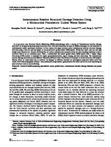
Figure 1: Deployment scheme of piezoelectric patches on aluminum plate used for testing 2.1 Sensor Diagnostics With the sensors attached to the plate, the consistency of the bonding and operating condition of the patches was determined using the sensor diagnostic technique. The sensor diagnostic technique involves gathering admittance measurements from each of the piezoelectric patches bonded to the plate over a specified range of frequencies. In this study, a range of 40 Hz - 100 kHz was used in order to completely cover the frequency range of interest. The slope of the imaginary part of the admittance vs. frequency curve for each of the piezoelectric devices, which is analogous to the capacitive value of the piezoelectric devices, is compared for consistency. Admittance measurements are also taken for a patch in a free-free state in order to develop a reference. The principle behind this technique is that patches with similar admittance slopes have similar bonding and operating conditions. Patches with an increased slope indicate a poor bonding condition; the extreme of which is the patch measured in the free-free condition. Patches with a decreased slope indicate a broken or otherwise degraded piezoelectric device. A detailed explanation of the sensor diagnostic technique used and the mathematical derivations supporting it can be found in references [10-11]. A plot of the admittance curves for a plate with a broken patch can be seen in Figure 2.
Imaginary Part of Admittance
Admittance Measurement from Piezoelectric Patches 1.2E-03
Free Patch Patch 1
1.0E-03
Patch 2
8.0E-04
Patch 3 Patch 4
6.0E-04
Patch 5
Broken Patch
4.0E-04 2.0E-04
Patch 6 Patch 7 Patch 8 Patch 9
0.0E+00 0.0E+00
2.0E+04
4.0E+04
6.0E+04 8.0E+04 Frequency (Hz)
1.0E+05
1.2E+05
Figure 2: Admittance measurements for plate with broken patch 7 If the patch that was identified as damaged in Figure 2 was used in an SHM application, it is likely that there would be a false detection of damage in the plate. A broken or poorly bonded patch would not transmit or receive the same amount of energy or consistency of signal as a patch with good operating and bonding conditions, which is detailed in the reference [11]. The plot of the admittance measurements from the initial piezoelectric patch deployment on the first plate used in this research can be seen in Figure 3. The sensor diagnostics of the initial deployment indicated that patch 2 was in a slightly deteriorated condition when compared to the other patches. There was also a slightly weaker bond between the plate and patch 7. Admittance Measurement from Piezoelectric Patches First Set on Plate 1 of 4 Imaginary Part of Admittance
1.2E-03
Free Patch Patch 1
1.0E-03
Patch 2
8.0E-04
Patch 3 Patch 4
6.0E-04
Patch 5 Patch 6
4.0E-04
Patch 7
2.0E-04
Patch 8 Patch 9
0.0E+00 0.0E+00
2.0E+04
4.0E+04
6.0E+04 8.0E+04 Frequency (Hz)
1.0E+05
1.2E+05
Figure 3: Initial deployment of piezoelectric patches on plate 1 indicating inconsistency of patch 2 and patch 7 In order to improve the consistency of the bonding condition of the piezoelectric devices, patches 2 and 7 were removed and replaced. The result of the sensor diagnostics taken from the plate after patches 2 and 7 were replaced can be seen in Figure 4. This plot shows consistency in the operating and bonding condition of all of the patches deployed on the plate. This consistency allows for the assumption that each piezoelectric patch will transmit and receive similar signals.
Admittance Measurement from Piezoelectric Patches Second Set on Plate 1 of 4 Imaginary Part of Admittance
1.2E-03
Free Patch Patch 1
1.0E-03
Patch 2
8.0E-04
Patch 3 Patch 4
6.0E-04
Patch 5 Patch 6
4.0E-04
Patch 7
2.0E-04
Patch 8 Patch 9
0.0E+00 0.0E+00
2.0E+04
4.0E+04
6.0E+04 8.0E+04 Frequency (Hz)
1.0E+05
1.2E+05
Figure 4: Final deployment of piezoelectric patches used for testing 2.2 Data Collection Technique In the test specimen described above, voltage data sets were taken for three sets of different length paths, as seen in Figure 5. The data sets were collected using a pitch-catch technique between the piezoelectric patches, through which each piezoelectric device acts as both a sensor and an actuator creating the paths seen in Figure 5. For example, a voltage signal would be passed through patch 1 which would strain the patch and excite a wave in the plate. Patch 2 would then be used as a sensor to measure the strain caused by the wave at that location. This strain is converted into a voltage by the piezoelectric patch, which is then recorded by the data acquisition system. A list of the actuator-sensor pairings used to develop the paths used for SHM can be seen in Table 1.
(a) Short straight path length
(b) Short diagonal path length
(c) Long diagonal path length
(d) Overall specimen coverage
Figure 5: Various path lengths used and total part coverage
Table 1: Actuator-sensor pairings used to develop SHM paths Short Straight Paths Actuator Sensor 1 2 1 4 2 3 2 5 3 6 4 5 4 7 5 6 5 8 6 9 7 8 8 9
Short Diagonal Paths Actuator Sensor 1 5 2 4 2 6 3 5 4 8 5 7 5 9 6 8
Long Diagonal Paths Actuator Sensor 1 6 1 8 2 7 2 9 3 4 3 8 4 9 6 7
2.3 Excitation of Lamb Waves In order to generate a plate wave that would produce a somewhat predictable response at the sensor locations, the desired properties of the excitation signal had to be determined. A burst sinusoidal waveform was selected to minimize the shock to the piezoelectric device when excited while still maintaining a signal at a discrete, selectable frequency. Dispersion curves were plotted in order to estimate what frequency should be used for the excitation. The dispersion curves were used to determine approximate wave speeds for both the symmetric and asymmetric modes of the lamb wave as well as the amount of variation that a small change in the plate (i.e. thickness, stiffness) would cause. These curves provide for an educated estimate for the appropriate frequency of the excitation signal. A range of frequencies was then selected and tested using the first plate studied. After preliminary testing a 5 V, 60 kHz burst waveform was selected for use as the actuator signal, and can be seen in Figure 6. 5 V, 60 kHz Burst Waveform Excitation Signal 5 4 3
Voltage (Volts
2 1 0 -1 -2 -3 -4 -5
0
500
1000
1500 Data Points
2000
2500
3000
Figure 6: Actuator signal used to excite piezoelectric patches The 5 V input was found to have the least amount of noise in the signal while still operating within the limits of the electrical equipment used. It should be noted that the 5 V burst waveform shown above is the excitation signal generated by MATLAB. This signal is sent through an amplifier before it reaches the piezoelectric patches. The actual voltage seen by the patches is approximately 15 V. When selecting the excitation frequency, signals with lower frequencies have larger wavelengths and reduced the systems’ overall sensitivity to detecting damage,
making higher frequency signals desirable. Lower frequencies, however, help maintain speeds of the A0 and S0 modes that result in little to no interaction between the first arrivals of the two modes at each sensor. This separation of arrival times helps to reduce the additive or diminishing effects caused by the interaction of the two modes. Additionally, it was found that at higher frequencies, there was a much larger variation between the signals recorded from different undamaged paths of equal length. These variations are caused by slight inconsistencies between path variables including sensor placement, among piezoelectric transducers, and between test specimen. A compromise was made and a frequency of 60 kHz was selected because of its balance between signal variation and sensitivity to damage. After the input signal frequency was selected, it was determined that the A0 mode would be used for analysis because of its higher sensitivity to damage over the S0 mode. The S0 mode, however, has several advantages including a higher wave propagation speed for the frequencies tested, resulting in no effects from reflections or A0 mode interference. The S0 mode is also relatively insensitive to change in input frequency and physical variations between paths. The negative aspect of the insensitivity to physical path variation is that it is also insensitive to damage. Based on the A0 mode’s higher sensitivity, it was selected for analysis. Similar results were found in a study by Thomas et al. [12] in the specific case of material loss in the specimen. 2.4 Testing Performed Several sets of data were acquired for the undamaged plate to determine test-to-test and path-to-path variability. After these undamaged sets of data were acquired, reversible damage in the form of industrial putty was applied to the plate which added mass and damping to simulate damage. The putty provided a removable damage case that could be moved to any location on the plate in order to establish the sensitivity of each path to damage and to test the signal processing algorithms which will be described in a later section of the paper. The putty is also useful for determining how close damage has to be to a path for the sensor to exhibit detectable signal variation. In order to determine the sensitivity of the technique to a real-world type of damage, corrosion was induced in the plate. In order to corrode the plate, saline solution was placed in a bottomless container that was sealed to the plate in order to control the area to be corroded. A small piece of aluminum was attached to the negative side of a power supply and placed in the solution acting as a cathode. A small voltage was applied to the plate forcing it to act as the sacrificial anode causing the plate to corrode. Several different corrosion cases were explored. The initial case studied involved corroding the plate in a small circle on a direct path at discrete depth intervals. This increase in depth was performed in an attempt to determine how severe the corrosion damage must be to produce detectable signal variation. The corrosion induced in the plate resulted in a final circular damage with 1.04 in (26.42 mm) diameter and 0.033 in (0.84 mm) depth. A concentric circle of less severe corrosion was later added around the initial small circle previously discussed. The concentric circle corrosion was induced to simulate the variations found in real-world corrosion damage. The concentric corrosion had a diameter of 1.84 in (46.74 mm) and a depth of 0.018 in (0.46 mm). The effects of non-circular damage were also explored by inducing an elliptical corrosion at the intersection of two of the short diagonal paths. This resulted in one of the signals traveling through the corrosion for a significantly longer distance than the other. The dimensions of the elliptical corrosion were 3.83 in (97.28 mm) long by 1.12 in (28.45 mm) wide with a depth of 0.023 in (0.58 mm). The final corrosion damage induced in the plate was placed in an area not directly crossed by one of the actuatorsensor paths. By locating damage out of the direct paths, the sensitivity of the signals to nearby damage can be determined. The off-path damage will also help to determine the density of sensors required to successfully locate damage in the plate. The corrosion induced to monitor off-path sensitivity was a circle with a 1.24 in (31.50 mm) diameter and a 0.02 in (0.51 mm) depth. A second plate was instrumented with the same pattern as the first plate and a cut was slowly induced in one of the short path lengths. The cut was made using a thin cutting wheel on the end of a Dremel tool. The depth of the cut was increased at discrete intervals until the back side of the plate was breached. After the final cut was made, the void in the plate was approximately 0.04 in (1.02 mm) wide and 0.8 in (20.32 mm) long. The second plate was used for assessing the sensitivity of the technique to the cut due to the large number of damaged locations in the first plate. When the majority of the paths are affected by the damage in the plate, the statistical approach used in this technique begins to fail. It becomes difficult to determine which paths represent an undamaged condition since there is no longer a clear trend. In practice, this technique will most likely work well on large structures with many similar paths in order to maintain an undamaged average that is not greatly affected by multiple damaged locations.
3. DATA PROCESSING TECHNIQUES In order to analyze the data collected in this study, two techniques were developed; both of which are used only on the first arrival of the A0 wave. The first of these two techniques involves a cross correlation analysis performed on the first A0 mode wave arrival for all paths of equal length. The second method utilizes the area under the power spectral density curve for each signal to monitor the energy transferred across each path. The data analysis code for both techniques was developed using MATLAB. The statistical nature of both of the analysis techniques requires that there be a reasonably large ratio of undamaged to damaged paths. This is especially true in the case of multiple damaged paths which will skew the statistical methods with which the instantaneous baseline measurements are created if enough undamaged paths are not present. A detailed description of each data processing technique is described below. 3.1 Detailed description of cross correlation analysis technique The first technique developed involves the cross correlation analysis of each signal from paths of equal length. This determines the degree to which two signals are linearly related. Using the analysis technique described below, paths with outlying characteristics can be recognized when compared to other paths of equal length. In the equations below, an example path “g” will be removed. The cross correlation value is first determined for all combinations of equal length paths. The function used to compute the cross correlation value allows for a phase shift to account for small differences in plate characteristics and sensor placement. The peak value in the cross correlation function is then found to determine how well signals correlate. The peak value “a” is subtracted from 1, causing outlying paths to have a higher value than that of a statistically common path. This decimal is squared to increase the difference between a statistically common path and an outlying path. The correlation for each path with all other equal length paths will then be summed (a total of 12 correlation coefficients for the short paths) causing any outlying paths to have a greater magnitude when plotted on a bar graph. This mathematical process can be seen in equation form as “e” in (1).
e(i ) = ∑ (1 − a(i ) ) n
2
(1)
i =1
The path with the least correlation (i.e. greatest distortion in shape) is removed and the cross correlation is again performed on the remaining paths. These cross correlation coefficients are then summed and scaled. Scaling is necessary for comparison purposes because the sums of these correlation values are of only the remaining paths (11 for the short paths). Because it is desired to find the percent difference between the correlation values of the original 11 paths while damage was present, and the final 11 paths where the damaged path has been removed, the final 11 paths must represent the addition of 12 numbers not the 11 that remain. The new cross correlation values are scaled by adding the average of the remaining values to the overall sum of the cross correlation values. When taking the average, the sum of the remaining numbers will be divided by one less than the number of remaining paths because there is a zero value representative of when each path is compared to itself. The summation and scaling of these values are shown as “b” and “c” in (2) and (3) respectively. The magnitude of these summed values is then plotted on a bar graph for comparison of the remaining paths. n −1
b(i ) = ∑ (1 − a(i ) )
(2)
b(i ) n−2
(3)
2
i =1
c(i ) = b(i ) +
The magnitudes of the summed correlation values from the remaining paths are then summed together, shown as “d” in (4). The magnitudes of all paths from the original cross correlation performed are also summed and the magnitude of the least correlated path is subtracted, shown as “f” in (5).
n −1
d = ∑ c(i )
(4)
⎛ n ⎞ f = ⎜⎜ ∑ e(i ) ⎟⎟ − e( g ) ⎝ j =1 ⎠
(5)
j =1
The percent difference between these two numbers is then calculated, shown mathematically in (6), to determine how much the removed path affected the initial cross correlation value. This path removal technique is repeated as many times as necessary until a relatively small percent difference is reached. When the desired percent difference is reached, the paths that were previously removed with a higher percent change can be designated as damaged.
⎛ f −d ⎞ ⎟⎟ × 100 %difference = ⎜⎜ f ⎝ ⎠
(6)
Using this technique it will be necessary to set a percent difference threshold for damage, but not an actual threshold for the numerical values found in the cross correlation. If a threshold for the cross correlation values was necessary, a baseline measurement would have to be taken in order to find the threshold for any structure on which this system is to be deployed. Since avoidance of a baseline measurement from the undamaged structure is a primary goal, it is desirable to use this percent difference method. 3.2 Detailed Description of Power Spectral Density Technique The technique developed involves the calculation of the power spectral density (PSD) for each signal acquired. The PSD is calculated using Welch’s averaged modified periodogram method of spectral estimation with no overlapping signal samples and a rectangular window. Once the PSD has been calculated for the first A0 mode arrival for each of the equal length paths, the area under each curve is determined using the trapezoid rule, giving the average power of the signal. The mean value of the average power for all equal length paths is then calculated. The mean power value is then compared to each individual path by calculating the percent difference as defined by (7). The percent difference is then calculated for each individual path as compared to the mean average power value. The percent difference is multiplied by negative one so that signals with a greater average power will show a positive percent difference and signals with a lower average power will show a negative percent difference.
percent difference(i ) =
mean power − power (i )
× (− 1)
(7)
mean power Through this technique, any signal that has a statistically increased or decreased average power can be identified and differentiated. This allows for recognition of both attenuated and amplified signals. Similar to the cross correlation method, a threshold on percent difference must also be set for the PSD technique. Again, this is not a threshold set on the actual average power values calculated, but on the percent difference of those values away from the mean. 4. EXPERIMENTAL RESULTS 4.1 Undamaged Plate The first few sets of data recorded on both of the plates used in this study were taken on undamaged plates. Typical undamaged time histories for each of the three path lengths can be seen in Figure 7.
Time HIstory Short Straight Path, Plate 1 - Undamaged
Time History Short Diagonal Path, Plate 1 - Undamaged
Path 1 to 2 Path 2 to 3
0.1
Path 2 to 5 Path 3 to 6 Path 4 to 5
0
Path 4 to 7
-0.2
Path 1 to 5
0.15
Path 2 to 4
0.1
Path 2 to 6 Path 3 to 5
0.05
Path 4 to 8
0
Path 5 to 7
-0.05
Path 5 to 9
Path 5 to 8
-0.1
Path 6 to 8
Path 6 to 9
-0.15
Path 5 to 6
-0.1
Voltage (V)
Voltage (V)
Path 1 to 4 0.2
Path 7 to 8 4000
4500
5000
5500
6000
6500
6000
Path 8 to 9
Data Point
6500
7000
7500
8000
8500
Data Point
(b) Short Diagonal Path
(a) Short Straight Path Time History Long Diagonal Path, Plate 1 - Undamaged
Path 1 to 6 Path 1 to 8
0.1
Path 2 to 7 Voltage (V)
0.05
Path 2 to 9 Path 3 to 4
0
Path 3 to 8 Path 4 to 9
-0.05
Path 6 to 7 -0.1 0.95
1
1.05
1.1
1.15
1.2
Data Point
4 x 10
(c) Long Diagonal Path
Figure 7: Time history plots for typical undamaged plate These undamaged time histories were used to determine the typical signal variation of each path length in order to help establish the sensitivity of the proposed instantaneous baseline technique. All of the data sets taken from undamaged cases were analyzed using both the cross correlation and PSD methods to help determine usual percent differences when no damage is present. The threshold on percent difference for each technique must be set significantly higher than any of the observed percent differences on the undamaged plates. Typical values of percent difference for the cross correlation method for short straight, short diagonal, and long diagonal paths are 20%, 26%, and 26%, respectively. The PSD method has shown typical percent difference values of 20%, 13%, and 30% for short straight, short diagonal, and long diagonal paths, respectively. Based on changes in the percent differences observed for a variety of damaged cases, it can be concluded that in the plate structures explored, increases of 10%-20% above the normal undamaged percentages indicate paths of questionable condition, and increases above 20% indicate damaged paths. 4.2 Removable Putty Damage Figure 8 (a) shows a photograph of the first aluminum plate with a large piece of removable silly putty plated between patches 2 and 3. The time domain plot of the data recorded from the plate during this test, as well as the results of the cross correlation and PSD analysis are also shown in Figure 8 (b)-(e). When placing a large piece of putty in a direct short straight path, the time signal recorded for the damaged path is severely attenuated when compared to the signals from the remaining undamaged paths. This result is demonstrated in Figure 8 (b). Although this visual based detection works well in this case, the signal may not always be distorted to this extent. Additionally, the visual method relies on human interaction to detect damage. For these reasons, the cross correlation and power spectral density methods were implemented. Upon analyzing the data using the cross correlation and PSD method we notice in Figure 8 (c) and (e) that path 2-3 shows significantly poor correlation and less power/frequency than the rest of the paths, respectively. Again these results visually show that path 2-3 is damaged; however, the visual method cannot be used for the same reasons as described previously, therefore, mathematical algorithms were developed to quantify the extent of damage detected using each method. First, using the cross correlation method a percent difference of 91.78% was found after removing path 2-3 from the data set. The modified correlation coefficients decreased significantly after removal of path 2-3, as seen by comparing Figures 8 (c) and (d). Next, the PSD method presents a -90.86%
difference between the average area under all of the PSD curves and the area under the damaged curve for path 2-3 using (7). Based on these results, both the cross correlation and PSD methods are able to confidently detect damage in the plate when a large piece of putty is placed in a direct short straight path. Additionally, the PSD method is able to show that the signal from path 2-3 is attenuated because of the negative percent difference found. Several other cases were studied involving removable putty damage with various putty sizes and locations. The results of these additional tests were used to help develop the two data processing methods used in this study and will not be detailed in this paper.
1
2
Time History Short Straight Path, Plate 1 - Silly Putty Between Patches 2 and 3
3
Path 1 to 2 Path 1 to 4
0.2
5
Path 2 to 5
6
0.1 Voltage (V)
4
8
Path 2 to 3 Path 3 to 6 Path 4 to 5
0
Path 4 to 7 Path 5 to 6
-0.1
9
Path 5 to 8 Path 6 to 9 Path 7 to 8
-0.2 4500
5000
5500
6000
6500
Path 8 to 9
Data Point
(b) Time history for short straight path lengths
(a) Photograph of removable putty damage
M odified C or r elation C oeffic ient
M odified C orr elation C oefficient
0.05 0.04 0.03 0.02 0.01 0 1-2 1-4 2-3 2-5 3-6 4-5 4-7 5-6 5-8 6-9 7-8 8-9
4.5 Path 1 to 2 Path 1 to 4
4
Path 2 to 3
3.5
0.04 0.03 0.02 0.01
Path 2 to 5 3
Path 3 to 6 Path 4 to 5
2.5
Path 4 to 7 Path 5 to 6
2
Path 5 to 8 1.5
Path 6 to 9
1
Path 7 to 8 Path 8 to 9
0.5
0 1-2 1-4 2-5 3-6 4-5 4-7 5-6 5-8 6-9 7-8 8-9 Path
Path
(c) Cross correlation analysis before removing path 2-3
Power Spectral Density Estimate -7 x 10 Short Straight Path, Plate 1 with Putty Between Patches 2 and 3
Cross Correlation Analysis Short Straight Path, Plate 1 with Putty Between Patches 2 and 3 Path 2-3 Removed from Data Set 0.05 Power/frequency (W/Hz)
Cross Correlation Analysis Short Straight Path, Plate 1 with Putty Between Patches 2 and 3
(d) Cross correlation analysis after removing path 2-3
0 0
2
4
6
8
10
Frequency (Hz)
12 4
(e) Power Spectral Density plot
Figure 8: Photograph and analysis results of plate 1 with putty placed between patches 2 and 3 4.3 Corrosion Damage with Increasing Depth Once it was shown that both the cross correlation and PSD methods were capable of detecting removable putty damage, permanent damage in the form of corrosion was induced onto the plate to better represent real-world damage. Corrosion is an extremely costly problem for industries and business sectors throughout the world and imparts a negative impact on these countries’ economies. In 1998, Congress funded the Department of Transportation and the Federal Highway Administration (FHWA) to estimate the total cost of corrosion on the U.S. economy and provide corrosion prevention guidelines. The final results of the survey estimated the extrapolated total direct corrosion cost to be $278 billion per year which is 3.14% of the gross domestic product in the United States [13]. The first type of corrosion damage investigated was a small circular pit of 1.04 in (26.42 mm) diameter in the middle of path 2-3 on plate 1. The same location was corroded multiple times at discrete depth intervals and data was recorded for each depth obtained. Figure 9 shows photographs of the initial and final corrosion sites. A table of depth values and the corresponding percent differences for the cross correlation and PSD techniques is
presented in Table 2. Additionally, a graph of that data that shows the trend of percent difference as a function of depth is shown in Figure 10 for both methods.
(a) Initial corrosion - 0.004 in (0.102 mm)
(b) Final corrosion - 0.033 in (0.838 mm)
Figure 9: Photographs of initial and final corrosion between patches 2 and 3 on plate 1 Damage Identification with Increasing Corrosion Depth 110
Table 2: Percent differences in path 2-3 for cross correlation and PSD methods with increasing corrosion depth
100
Power Spectral Density
90
Cross Correlation
Depth (in) / (mm)
Percent Difference (%)
0.004 / 0.102 0.007 / 0.178
Cross Correlation N/A N/A
PSD 36.12 39.3
0.016 / 0.406 0.016 / 0.406 0.019 / 0.483 0.021 / 0.533 0.024 / 0.610
N/A N/A N/A N/A N/A
52.45 62.21 68.07 71.65 56.03
0.029 / 0.737 0.033 / 0.838
54.22 98.48
19.11 80.06
Percent Difference (%)
80 70 60 50 40 30 20 10 0 0
0.005
0.01
0.015
0.02
0.025
0.03
0.035
Depth (in)
Figure 10: Graphical representation of percent difference trend in path 2-3 with increasing corrosion depth for both data analysis techniques
As seen in Table 2, the cross correlation method does not indicate percent differences for the first seven corrosion depths. This is because paths other than path 2-3 have the highest modified correlation coefficient for these depths; therefore, the cross correlation method is unable to detect damage for these conditions. As the corrosion depth increases, however, to 0.029 in (0.737 mm), the percent difference found using cross correlation jumps suddenly to 54.22%, and for a depth of 0.033 in (0.838 mm) a percent difference of 98.48% is calculated. The conclusion can be made that the cross correlation method is unable to detect small circular corrosion damage in a direct short straight path for depths of less than around 0.027 in (0.686 mm). Upon analyzing the same data with the PSD method, much better results were obtained for most of the depth values tested. At the first stage of corrosion with a depth of 0.004 in (0.102 mm), the PSD analysis found a percent difference of 36.12% which claims that the path has questionable condition. When the corrosion damage reaches a depth of just 0.016 in (0.406 mm), a percent difference of 52.45% is calculated and the path can be called damaged. An interesting trend, however, can be seen in Figure 10. When the corrosion depth increases above 0.021 in (0.533 mm), the percent differences begin to drop. At a depth of 0.029 in (0.737 mm), the PSD method only calculates a percent difference of 19.11%, which is similar to the values obtained in an undamaged plate. Further increasing the depth, however, to 0.033 in (0.838 mm) results in a significant increase in percent difference to 80.06%. Although a significant drop in percent difference was observed, it is believed that this trend
will only be observed over a small range of depths. To further examine this trend, the time histories for each depth were investigated and it was observed that as the depth increased from 0.004 in (0.102 mm) to 0.021 in (0.533 mm), the signal amplitude increased. Although this result is significantly different from the attenuation observed when putty was attached to the plate, this signal amplification associated with corrosion has been observed in other research [12]. Once the depth increased beyond 0.021 in (0.533 mm), the time history signal began to attenuate. At a depth of 0.029 in (0.737 mm), where the PSD method was unable to detect the damage, the amplitude of the damaged signal was approximately equal to the amplitude of the undamaged signals, hence the inability of the PSD technique to identify damage. As the depth increased to 0.033 in (0.838 mm), the attenuation continued to increase and the PSD method began to detect the damage again. Examining the data recorded for corrosion with increasing depth in the direct path 2-3 shows that combining both the cross correlation and PSD techniques results in detection of the corrosion for any depth above 0.016 in (0.406 mm). The fact that the cross correlation technique begins to identify the damage when the PSD method no longer does shows the importance of using both methods for each test. The cross correlation and PSD techniques identify damage based on different changes observed in the data, and the combination of both techniques allows for detection based on attenuation, amplification, frequency shift, and shape change. 4.4 Concentric Circle Corrosion The data processing methods developed in this study were successful in detecting a fairly uniform circular corrosion pit, however, natural corrosion is often more irregular than the initial corrosion studied. A concentric circle of less severe corrosion, therefore, was added around the initial small circle in path 2-3 on plate 1 to better represent a real-world damage case. Two photographs of the concentric circle corrosion are presented in Figure 11. The larger circle had a final diameter of 1.84 in (46.74 mm) and a depth of 0.018 in (0.46 mm), where the diameter and depth of the smaller circle remained at 1.04 in (26.42 mm) and 0.033 in (0.838 mm), respectively.
Figure 11: Photographs of plate 1 with concentric corrosion damage between patches 2 and 3 The results of the data analysis on the short straight paths using the cross correlation and PSD methods show a small decrease in the percent differences of path 2-3 when compared to the results from the small circular pit described in the previous section. Before the concentric circle was added to the plate, the small circle showed damage percentages of 98.48% and 80.06% for cross correlation and PSD, respectively. Once the larger circle was added, those percentages dropped to 96.80% and 71.62% for cross correlation and PSD, respectively. The results of the cross correlation analysis appear to be insensitive to the addition of the larger circle, and the PSD technique appears to be less sensitive to the damage. Although the ability of the PSD technique to detect damage seems to decrease with the addition of the larger circle, investigating the actual PSD curves reveals additional information that may be useful in detecting damage. Figure 12 presents a graph of the PSD curves of path 2-3 for the damage both before and after the addition of the concentric corrosion.
-8 x 10
Power Spectral Density Estimate Short Straight Path 2-3 Comparison of Single Circle and Concentric Circle Corrosion
7 Test 23 - Single Circular Corrosion Test 24 - Concentric Corrosion Damage
Power/Frequency (W/Hz)
6
5
4
3
2
1
0 0
2
4
6
8
10
12
Frequency (Hz)
4 x 10
Figure 12: PSD Plot of path 2-3 before and after the concentric corrosion damage From Figure 12, it is observed that adding the larger circle of corrosion caused the distribution of power in the signal to shift towards a lower frequency range. This means that the time history recorded for the concentric corrosion had higher amplitude at slightly lower frequencies than the time history recorded for the small circle. Although shifts in frequency of PSD curve are not currently used in the damage detection algorithms developed in this study, they may prove useful as damage detection metrics and should be further investigated. Upon analyzing the data recorded for the long diagonal paths, however, a significant increase is found in the percent difference calculated using the cross correlation method in path 3-4 with the addition of concentric damage. Before the larger circle of corrosion was added to the plate, path 3-4 gave a percent difference of 36.07% using the cross correlation analysis. After the concentric circle was added, the cross correlation method gave a percent difference of 71.46% for path 3-4. The result of the cross correlation for this case is presented in Figure 13. Although the 36.07% calculated for just the small circle can indicate path 3-4 as questionable, the value is barely above the threshold. With the addition of the larger circle, the cross correlation method can confidently indicate path 3-4 as a damaged path. The fact that the concentric circle damage had a larger diameter helps to explain this observation. With the small corrosion, reflections off of the damage for path 3-4 were probably minor, but because the edge of the damage was much closer to path 3-4 when the concentric circle was added, the likelihood of reflections altering the signal is much greater.
Modified Correlation Coefficient
Cross Correlation Analysis Long Diagonal Path, Plate 1 with Concentric Corrosion Between Patches 2 and 3 0.06 0.05 0.04
0.03
0.02 0.01
0 1-6
1-8
2-7
2-9
3-4
3-8
4-9
6-7
Path
Figure 13: Cross correlation analysis for concentric circle damage in path 2-3 4.5 Elliptical Corrosion The ability of the instantaneous baseline SHM technique to detect non-circular corrosion damage was also explored by inducing an elliptical corrosion at the intersection of two of the short diagonal paths on plate 1. The elliptical corrosion had a length of 3.83 in (97.28 mm) and a width of 1.12 in (28.45 mm). Two discrete depths of
0.019 in (0.483 mm) and 0.023 in (0.584 mm) were tested. Figure 14 shows two photographs of the elliptical corrosion induced on the plate.
1
2
3
4
5
6
7
8
9
(a) Overall view of plate 1 with elliptical damage in path 5-7
(b) Close up view of elliptical damage in path 5-7
Figure 14: Photographs of plate 1 with elliptical damage between patches 5 and 7 The effects of non-circular damage on the short diagonal paths were determined by analyzing the data recorded with elliptical corrosion in path 5-7. When investigating the results of the cross correlation analysis, percentages around 25% were calculated for both depths in paths 5-7 and 4-8, both of which pass through the damage. When comparing these results to those found for the small corrosion between patches 2 and 3, the short straight paths could not detect the small corrosion at these depth levels either. The conclusion is reinforced that at depths below 0.027 in (0.686 mm), the cross correlation method is unable to detect most corrosion damage. The PSD method was, however, able to detect the damage for both depths. Similar to the trend observed for small corrosion in path 2-3, the time histories of paths 5-7 and 4-8, shown in Figure 15, showed both amplification and attenuation depending on the depth of the corrosion, however, path 5-7 showed a different trend when compared to path 4-8. As the depth increased from 0.019 in (0.483 mm) to 0.023 in (0.584 mm), the percent difference values for path 5-7 decreased from 50.35% to 29.46%. Also, at the first depth level, path 5-7 showed the highest percentage, but at the second depth level, path 4-8 had the highest percentage and path 5-7 had the second highest. When investigating path 4-8, the PSD calculation for the first depth finds paths other than 4-8 to have the highest percentages. At the second depth level, however, path 4-8 has the highest percent difference at 53.12%. The results from the PSD analysis combined with observing the time histories shown in Figure 15, allows trends to be estimated not only with respect to depth, but with respect to length of damage as well. The difference between paths 5-7 and 4-8 is that path 5-7 sees damage with a length of 3.83 in (97.28 mm) and path 4-8 sees damage with a length of 1.12 in (28.45 mm). When compared to the trend observed for small corrosion, shown in Figure 10, it can be inferred that at these depth values, the longer damage of path 5-7 puts it in the downward portion of the curve where the shorter damage of path 4-8 is in an earlier part of the curve where the signal gains amplitude with increasing corrosion depth. Looking at the time histories shown in Figure 15, this inference can be validated. As the corrosion depth increases, the amplitude of the signal from path 5-7 decreases and the amplitude of the signal from path 4-8 increases. The fact that the two paths appear to be in different locations along the curve suggests that changing the length of the damage may have a similar trend as increasing the depth, however, more research needs to be done to verify this conclusion.
Time History Short Diagonal Path, Plate 1 - 0.019 in Deep Oblong Corrosion Between Patches 5 and 7 0.2
Time History Short Diagonal Path, Plate 1 - 0.023 in Deep Oblong Corrosion Between Patches 5 and 7
Path 1 to 5 Path 2 to 4
0.15
0.2
Path 1 to 5
0.15
Path 2 to 4 Path 2 to 6
Path 2 to 6 Path 3 to 5
0.1
Path 3 to 5
0.1
Path 4 to 8
Path 4 to 8 Path 5 to 7 Path 5 to 9 Path 6 to 8
0 -0.05
Path 5 to 7
0.05 Voltage (V)
Voltage (V)
0.05
Path 5 to 9 Path 6 to 8
0 -0.05 -0.1
-0.1
-0.15 -0.15
-0.2 -0.2 6500
7000
7500
8000
8500
6500
7000
7500
8000
8500
Data Point
Data Point
(a) Time history for 0.019 in (0.483 mm) depth
(b) Time history for 0.023 in (0.584 mm) depth
Figure 15: Time histories for various depth elliptical corrosion damage in path 5-7 4.6 Off-Path Corrosion The last type of corrosion damage investigated was located off of any of the direct paths. The instantaneous baseline technique was shown to successfully locate both removable putty and corrosion damage when the damage site is located directly between two patches; however, it was also necessary to evaluate the ability to detect off-path damage. A circular pit of corrosion measuring 1.24 in (31.50 mm) in diameter and 0.02 in (0.51 mm) in depth was created slightly off of path 6-9 as seen in Figure 16.
1
2
3
4
5
6
7
8
9
(a) Overall view of plate 1 with offpath damage in path 6-9
(b) Close up view of off-path damage in path 6-9
Figure 16: Photographs of plate 1 with off-path damage between patches 6 and 9 Examining the results of the cross correlation analysis for data collected with off-path damage shows the ability to detect this damage case. The data recorded for off-path damage is, however, affected by the fact that both the concentric and elliptical damage sites were present in the plate when recording data. When analyzing the data for the short straight paths, path 2-3 shows the largest percent difference of 87.88% because of the concentric damage. Path 6-9, however, does show the second highest percent difference at 59.41% once path 2-3 is removed, which is high enough to confidently indicate damage. The result of the cross correlation calculation with path 2-3 removed from the data set is presented in Figure 17 and clearly shows path 6-9 as damaged. The short diagonal and long diagonal paths, on the other hand, do not indicate damage, most likely because of the effects
of the other damage sites on the data. Additionally, the short diagonal and long diagonal paths may not have sufficient sensitivity to detect off-path damage. Cross Correlation Analysis -3 Short Straight Path, Plate 1 with Off-Path Damage Between 6-9 Path 2-3 Removed from Data Set x 10 4
Modified Correlaiton Coefficient
3.5 3 2.5 2 1.5 1 0.5 0 1-2 1-4 2-5 3-6 4-5 4-7 5-6 5-8 6-9 7-8 8-9 Path
Figure 17: Cross correlation analysis for off-path damage in path 6-9 after removing path 2-3 Analyzing the percent differences calculated with the PSD technique shows that the short straight paths are unable to detect the off-path damage. Path 6-9 using the PSD method does not appear as one of the paths with the highest percent difference. Additionally, the short diagonal paths do not indicate the off-path damage. Again, this may have to do with the interaction of the other two corrosion sites on the data recorded. The long diagonal paths, on the other hand, easily indicate path 2-9 as damaged. Plots of the time history and PSD result for the long diagonal paths are presented in Figure 18. A percent difference of 104.88% is calculated for path 2-9. Combining these results with those found for path 3-4 when analyzing the concentric circle corrosion, the long diagonal paths seem to be most sensitive to damage that is not in a direct path, but slightly away from the path. A possible reason behind this is that reflections off of the damage may add to the first A0 mode signal. Both cases indicate that the power in the signal increased significantly over the undamaged paths because of the positive percent difference in the PSD calculations. These results confirm that the energy in the wave is increasing as it passes by the corrosion damage, hence reflections may be adding to the signal. Time History Long Diagonal Path, Plate 1 - Off-Path Corrosion Between Patches 6 and 9
Power Spectral Density Estimate Long Diagonal Path, Plate 1 with Off-Path Corrosion Between Patches 6 and 9 -7 x 10 Path 1 to 6 2 Path 1 to 8
Path 1 to 6 0.1
Path 1 to 8 Path 2 to 7
Voltage (V)
Path 3 to 4 Path 3 to 8 Path 4 to 9
0
Path 6 to 7 -0.05
Path 2 to 7 Power/frequency (W /Hz)
Path 2 to 9
0.05
Path 2 to 9
1.5
Path 3 to 4 Path 3 to 8 Path 4 to 9
1
Path 6 to 7 0.5
-0.1
0 0.9
0.95
1
1.05
1.1
1.15
1.2
1.25
Data Point
(a) Time history of long diagonal paths with corrosion in path 2-9
1.3
1.35
1.4 4 x 10
0
2
4
6
8
Freuency (Hz)
(b) PSD plot of long diagonal paths with corrosion in path 2-9
Figure 18: Damage identification in path 2-9 for off-path corrosion
10
12 4 x 10
4.7 Cut Damage The final type of damage explored in this study involved slowly inducing a cut between patches 1 and 2 on plate 2. Seven discrete depth intervals were created with a final cut size of approximately 0.04 in (1.02 mm) wide and 0.8 in (20.32 mm) long. Figure 19 shows photographs of the plate after the final cut was made. Data sets were recorded at each depth. Upon analyzing all of the data using the cross correlation method, the first five depth levels gave percent differences of around 20%, which is about the same level as an undamaged case. Once the cut was almost through the plate, a percent difference of 48.42% was calculated for the sixth cut depth. The seventh data set, taken when the cut was through the entire thickness of the plate, yielded a percent difference of 65.32%, easily detecting the damage. The PSD method gave results similar to those obtained using the cross correlation method. For the first six cut depths, the PSD technique calculated percent differences of around 20%, again similar to results from undamaged cases. The seventh cut, however, produced a percent difference of 50.77%, which clearly indicated damage. Based on these results, it can be concluded that the cross correlation and PSD data processing methods are able to detect this type of cut damage in a short straight direct path only when the depth of the crack is nearly through the thickness of the plate.
1
2
3
4
5
6
7
8
9
(a) Overall view of plate 2 with cut damage in path 1-2
(b) Close up view of cut damage in path 1-2
Figure 19: Photographs of plate 2 with cut damage between patches 1 and 2 5. DISCUSSION The techniques discussed in the preceding sections have been shown to be successful in detecting damage in the two aluminum plates studied. With the combination of the power spectral density and cross correlation approaches, all damaged locations were identified. There are, however, some limitations that have been discovered while performing this research and data analysis. The statistical nature with which the instantaneous baseline is developed puts significant limitations on the number of damaged paths that can be identified. If the ratio of damaged paths to undamaged paths is too high, both techniques will begin to show scatter in the signals recorded, which could skew the statistical average from representing that of an undamaged path. After analyzing the data from this study, it was found that a 4:1 undamaged to damaged ratio would be the smallest relationship that could be used to successfully assess the true state of the plate. Higher ratios produced much better results and a clearer indication of damage, since the statistical average is much less affected by the outlying paths. If this ratio falls below 4:1, it is still possible to confidently identify the plate as damaged, but there are limitations on the confidence with which damaged locations can be pinpointed. There will also be greater physical variations in real-world structures that will affect the percent difference thresholds set in order to identify damaged paths. The plates studied in this research were square aluminum plates with no significant structural variations aside from the damages induced throughout the investigation. Real-world structures will contain greater complexities such as fasteners and geometrical changes. These structural dissimilarities will cause the undamaged paths to show
more variation resulting in a lower sensitivity to damage because the percent difference threshold must be increased to accommodate for these variations. When processing the data for the corrosion and cut damage types, several issues arose that affected the performance of the two data analysis techniques implemented in this study. When increasing the depth of the corrosion damage on the short direct path length, it was noticed that the amplitude of the signal initially increased when compared to that of the undamaged paths. This amplification trend continued, but eventually the signal peaked. Further corrosion into the plate depth caused the signal to become increasingly attenuated. When analyzing the data using the power spectral density method, for almost all depth levels, this does not pose any problems as it can detect any increase or decrease in amplitude. The problem arises as the signal begins attenuating from the peak of its amplified state, eventually returning to its original amplitude which is equal to that of an undamaged path. At and around this point, the power spectral density method is not sensitive enough to detect the damage. It is for this reason that the cross correlation method must also be employed. At the point where the undamaged and damaged paths have similar amplitude there is a noticeable shape change in the damaged signal. The cross correlation technique picks up on this shape change and identifies the damaged path. Although the combination of these two methods successfully detected the damage across the corrosion depth values tested, this issue should be further explored to determine how corrosion affects wave propagation. It was also observed that as the depth of cut in the short path of plate 2 was increased, there was very little change in the recorded signal. It was not until the cut had nearly passed through the plate, that either analysis method could detect any significant change in the signal. This shows that the two techniques are not sensitive enough to locate this type of damage easily. This issue could be explored further by varying the size and shape of the cut or attempting to develop other, more sensitive analysis methods for the data recorded. 6. FUTURE WORK The research performed in this study has shown that it is possible to detect damage in an aluminum plate by using outlying signal characteristics to identify damaged paths. Although this concept has been shown to work on the specimens tested, there are several areas that must be further explored before this technique is implemented in an SHM system in a real-world structure. In order to understand how the recorded signals will be affected by different types and magnitudes of damage, wave propagation in damaged plates must be modeled. This modeling will help to prove the accuracy of the results obtained. It will also help with the understanding of the amplification and attenuation behavior patterns seen in the corrosion damage cases. Additionally, it will be necessary to explore other types and variations of damage including fatigue cracks and various corrosion shapes. Complex structures more resembling those where an SHM system might be employed should also be tested. This would include various geometries and the addition of fasteners and stiffeners that could be seen in a typical aluminum plate application. Future study should also include research on the variation of the percent difference thresholds for the analysis techniques. As structures become more complicated, it is likely that there will be more variation in undamaged path signal properties which will have to be taken into account when setting threshold values. This issue may be somewhat alleviated by intelligent placement of sensors. If sensors are placed in such a way that the common features of the structure are monitored by equal length paths with similar features between the sensors, undamaged path variation may be minimized. There should also be an in-depth look into the data processing of the signals recorded. Different methods should be employed to determine if there are more sensitive techniques than those used in this study. Several possibilities exist for data analysis including a peak pick for the PSD to determine if the frequency of the recorded signal has varied from that of an undamaged case. The cross correlation could also be performed on the PSD plots for the graphs to determine any broad band frequency shifts. 7. CONCLUSION An array of nine piezoelectric devices used as sensors and actuators were used for Lamb wave based SHM in such a way that several common features of undamaged sensor-actuator paths were obtained instantaneously. These paths identified as being undamaged were then used in place of a baseline measurement for the detection of damaged paths. This technique relies on the use of sensor diagnostics to minimize false damage identification and signal distortion caused by faulty or poorly bonded piezoelectric devices. Removable putty, corrosion, and cut damage were successfully detected in the aluminum plate specimens tested by analyzing the results from both a cross correlation and a power spectral density data processing method. Although the techniques used
were able to detect the damages induced in the plates in this study, more complex structures and types of damage will have to be explored before the implementation of instantaneous baseline techniques into SHM systems in real-world settings. 8. ACKNOWLEDGEMENTS The authors would like to thank Dr. Charles Farrar at Los Alamos National Laboratory for organizing the 2006 Los Alamos Dynamic Summer School. Funding for the summer school was provided by the Engineering Institute at Los Alamos National Laboratory. Finally, the authors would like to thank The Mathworks, Inc. for providing the software necessary to complete this project (MATLAB numerical analysis software). 9. REFERENCES [1] Inman, D.J., Farrar, C.R., Lopes Jr., V., and Valder Jr., S., “Damage Prognosis for Aerospace, Civil and Mechanical Systems,” John Wiley & Sons, Ltd., West Sussex, England, 2005. [2] Badcock R.A. and Birt, E.A., “The Use of 0-3 Piezocomposite Embedded Lamb Wave Sensors for Detection of Damage in Advanced Fiber Composites,” Smart Materials and Structures, Vol. 9, No. 2, pp. 291-297, 2000. [3] Giurgiutiu, V., Zagarai, A., and Bao, J.J., “Piezoelectric Wafer Embedded Active Sensors for Aging Aircraft Structural Health Monitoring,” International Journal of Structural Health Monitoring, Vol. 1, pp. 41-61, 2002. [4] Ihn, J.B. and Chang, F.K., “Detection and monitoring of hidden fatigue crack growth using a built-in piezoelectric sensor/actuator network: II. Validation using riveted joints and repair patches,” Smart Materials and Structures, Vol. 13, No. 3, pp. 621-30, 2004. [5] Kessler, S.S., Spearing, S.M., and Soutis, C., “Damage Detection in Composite Materials using Lamb Wave Methods,” Smart Materials and Structures, Vol. 11, No. 2, pp. 269-278, 2002. [6] Sohn, H., Park, G., Wait, J.R., Limback, N.P., and Farrar, C.R., “Wavelet-based Signal Processing for Detecting Delamination in Composite Plates,” Smart Materials and Structures, Vol. 13, No. 1, pp. 153-160, 2004. [7] Wilcox, P.D., Lowe, M.J. S., and Cawley, P., “Omni-directional Guided Wave Inspection of Large Metallic Plate Structures Using an EMAT Array”, IEEE Trans. on Ultrason. Ferroelec. and Freq. Cont. Vol. 52, pp. 653665, 2005. [8] Wilcox, P.D., “Omni-directional Guided Wave Transducer Arrays for the Rapid Inspection of Large Areas of Plate Structures”, IEEE Trans. on Ultrason. Ferroelec. and Freq. Cont. Vol. 50, pp. 699-709, 2003. [9] Viktorov, I.A., “Rayleigh and Lamb Waves,” Plenum Press, New York, 1967. [10] Park, G., Farrar, C.R., Rutherford, C.A., and Robertson, A.N., “Piezoelectric Active Sensor Self-diagnostics using Electrical Admittance Measurements,” ASME Journal of Vibration and Acoustics, Vol. 128, No. 4, pp. 469476, 2006. [11] Park, G., Farrar, C.R., Lanza di Scalea, F., and Coccia, S., “Performance Assessment and Validation of Piezoelectric Active Sensors in Structural Health Monitoring,” Smart Materials and Structures, Vol. 15, pp 16731683, 2006. [12] Thomas, D., Welter, J., and Giurgiutiu, V., “Corrosion Damage Detection with Piezoelectric Wafer Active Sensors,” Proceedings of SPIE - The International Society for Optical Engineering, v 5394, Health Monitoring and Smart Nondestructive Evaluation of Structural and Biological Systems III, pp. 11-22, 2004. [13] Virmani P. Corrosion cost and Preventive Strategies in the United States, Publication No. FHWA-RD-01-156 Washington, DC: FWHA, 2002.