Internet Search Assistant based on the Random Neural Network
Thesis submitted for the Degree of Doctor of Philosophy of the University of London and the Diploma of Imperial College
April 2018 Supervisor: Professor Erol Gelenbe
Guillermo Serrano Bermejo (Will Serrano)
[email protected] Intelligent Systems and Networks Group Electrical and Electronic Engineering Department Imperial College London
This work is on my own and else is appropriately referenced.
‘The copyright of this thesis rests with the author and is made available under a Creative Commons Attribution Non-Commercial No Derivatives licence. Researchers are free to copy, distribute or transmit the thesis on the condition that they attribute it, that they do not use it for commercial purposes and that they do not alter, transform or build upon it. For any use reuse or redistribution, researches must make clear to others the licence terms of this work’
Page 2 of 246
You
Acknowledgments Page
Page 3 of 246
Blank Page
Page 4 of 246
Table of Contents Abstract ............................................................................................................12 1
Introduction ............................................................................................13
1.1
Research Proposal ................................................................................... 14
1.2
Related Work .......................................................................................... 15
1.3
Summary of Contributions ........................................................................ 21
1.4
Summary of Publications .......................................................................... 23
2
Web Search .............................................................................................24
2.1
Internet Assistants .................................................................................. 24
2.2
Web Search Engines ................................................................................ 26
2.3
Metasearch Engines ................................................................................. 27
2.4
Web result clustering ............................................................................... 30
2.5
Travel Services ....................................................................................... 33
2.6
Citation Analysis ..................................................................................... 36
3
Ranking ...................................................................................................38
3.1
Ranking Algorithm ................................................................................... 38
3.2
Relevance Metrics ................................................................................... 43
3.3
Learning to Rank ..................................................................................... 48
4
Recommender Systems ...........................................................................50
4.1
Recommender System Types .................................................................... 50
4.2
Recommender System Relevance Metrics ................................................... 51
4.3
Recommender System Model .................................................................... 53
5
The Random Neural Network ...................................................................54
5.1
Neural Networks ..................................................................................... 54
5.2
Deep Learning ........................................................................................ 55
5.3
G-Networks ............................................................................................ 56
5.4
The Random Neural Network .................................................................... 58
5.5
The Deep Learning Cluster Random Neural Network .................................... 67
5.6
Random Neural Network Extensions .......................................................... 77
5.7
Random Neural Network Applications ......................................................... 79
6
Internet Search Assistant Model .............................................................87
Page 5 of 246
6.1
Intelligent Search Assistant Model ............................................................. 87
6.2
Result Cost Function ................................................................................ 88
6.3
User iteration .......................................................................................... 91
6.4
Dimension Learning ................................................................................. 94
6.5
Gradient Descent Learning ....................................................................... 96
6.6
Reinforcement Learning ........................................................................... 97
7
Unsupervised Evaluation .........................................................................99
7.1
Implementation ...................................................................................... 99
7.2
Spearman's Rank Correlation Coefficient .................................................. 101
7.3
Google Search ...................................................................................... 101
7.4
Web Search Evaluation .......................................................................... 104
7.5
Metasearch Evaluation ........................................................................... 107
8
User Evaluation – First Iteration ...........................................................111
8.1
Implementation .................................................................................... 111
8.2
Quality Metric ....................................................................................... 113
8.1
Google Search – Result Cost Function ...................................................... 113
8.2
Web Search – Result Cost Function.......................................................... 115
8.3
Google Search - Fixed Query – Relevant Centre Point ................................ 116
8.4
Google Search – Open Query - Relevant Centre Point ................................ 117
9
User Evaluation – Learning algorithms ..................................................119
9.1
Quality Metric ....................................................................................... 119
9.2
Web Search Evaluation .......................................................................... 120
9.3
Academic Database Evaluation ................................................................ 128
9.4
Recommender System Evaluation............................................................ 141
10
User Evaluation – Deep Learning ...........................................................158
10.1
Implementation .................................................................................... 159
10.2
Evaluation ............................................................................................ 159
10.3
Experimental Results ............................................................................. 161
11
Conclusions ...........................................................................................168
12
References ............................................................................................171
Appendix ........................................................................................................189 A ISA Screen shots ............................................................................................ 189
Page 6 of 246
B Unsupervised Evaluation .................................................................................. 190 C User Evaluation – First Iteration ....................................................................... 191 D User Evaluation – Learning Algorithms .............................................................. 201 E User Evaluation – Deep Learning ...................................................................... 238
Page 7 of 246
List of Figures Figure 1: Web search engine architecture ................................................................26 Figure 2: Metasearch services model ......................................................................28 Figure 3: Metasearch engine architecture ................................................................29 Figure 4: Web Cluster Engine Architecture ...............................................................31 Figure 5: Traditional travel services model ...............................................................34 Figure 6: Online travel services model .....................................................................35 Figure 7: Learning to Rank Model ...........................................................................49 Figure 8: Recommender system architecture ...........................................................50 Figure 9: Common types of Recommender systems ..................................................51 Figure 10: Recommender system model ..................................................................53 Figure 11: Artificial Neural Network – Recurrent and feed forward models ...................54 Figure 12: Artificial Neural Network – Deep Learning model .......................................56 Figure 13: Random Neural Network: Principles .........................................................59 Figure 14: Random Neural Network: Model ..............................................................60 Figure 15: Random Neural Network: Theorem ..........................................................61 Figure 16: Random Neural Network: Gradient Descent learning ..................................63 Figure 17: Random Neural Network: Gradient Descent iteration .................................64 Figure 18: Random Neural Network: Reinforcement Learning .....................................66 Figure 19: Random Neural Network: Reinforcement iteration .....................................67 Figure 20: Cluster Random Neural Network: Principles ..............................................69 Figure 21: Cluster Random Neural Network: Model ...................................................70 Figure 22: Single Cluster Random Neural Network: Theorem .....................................70 Figure 23: Multiple Cluster Random Neural Network: Theorem ...................................72 Figure 24: Cluster Random Neural Network: Gradient Descent learning .......................75 Figure 25: Cluster Random Neural Network: Gradient Descent iteration ......................76 Figure 26: The Random Neural Network with a Management Cluster ...........................77 Figure 27: Internet Search Assistant Model ..............................................................88 Figure 28: Intelligent Search Assistant User Iteration ................................................93 Figure 29: Intelligent Search Assistant Dimension Learning .......................................96 Figure 30: Intelligent Search Assistant Model – Gradient Descent Learning ..................97 Figure 31: Intelligent Search Assistant Model – Reinforcement Learning ......................98 Figure 32: ISA Client side implementation ............................................................. 100 Figure 33: ISA Client interface ............................................................................. 100 Figure 34: Google Search evaluation ..................................................................... 104 Figure 35: Web search evaluation – Average Values ............................................... 106
Page 8 of 246
Figure 36: Metasearch Evaluation – Average Values ................................................ 110 Figure 37: ISA Server implementation .................................................................. 112 Figure 38: ISA Server interface ............................................................................ 112 Figure 39: Google Search – Result Cost Function .................................................... 114 Figure 40: Web Search – Result Cost Function ....................................................... 115 Figure 41: Google Search - Fixed Query – Relevant Center Point .............................. 117 Figure 42: Google Search – Open Query - Relevant Center Point .............................. 118 Figure 43: ISA Web Search interface..................................................................... 121 Figure 44: Web Search evaluation – Gradient Descent - Average Values.................... 122 Figure 45: Web Search evaluation – Gradient Descent - Improvement ...................... 122 Figure 46: Web Search evaluation – Reinforcement Learning - Average Values .......... 124 Figure 47: Web Search evaluation – Reinforcement Learning – Improvement............. 124 Figure 48: Web Search evaluation – Evaluation between learnings ........................... 125 Figure 49: Relevance Metric Evaluation – Gradient Descent ..................................... 127 Figure 50: Relevance Metric Evaluation – Reinforcement Learning ............................ 127 Figure 51: ISA Academic Database interface .......................................................... 128 Figure 52: Database evaluation – Gradient Descent - Average Values ....................... 130 Figure 53: Database evaluation – Gradient Descent – Improvement ......................... 130 Figure 54: Database evaluation – Reinforcement Learning - Average Values .............. 132 Figure 55: Database evaluation – Reinforcement Learning - Improvement ................. 132 Figure 56: Database evaluation – Evaluation between learnings ............................... 133 Figure 57: Database Evaluation - Quality order by ISA ............................................ 134 Figure 58: Database Evaluation - Improvement order by ISA ................................... 135 Figure 59: Database Evaluation - Quality order by Academic Database ...................... 136 Figure 60: Database Evaluation - Improvement order by Academic Database ............ 136 Figure 61: Database Evaluation - Quality ISA and Online Academic Database ............ 138 Figure 62: Database Evaluation - Improvement ISA and Academic Database ............. 138 Figure 63: Relevance Metric Evaluation – Gradient Descent ..................................... 140 Figure 64: Relevance Metric Evaluation –Reinforcement Learning ............................. 141 Figure 65: ISA Recommender - Film interface ........................................................ 143 Figure 66: Recommender Evaluation – Film Database ............................................. 145 Figure 67: Recommender Evaluation - Improvement – Film Database ....................... 145 Figure 68: ISA Recommender – Trip Advisor interface ............................................. 147 Figure 69: Recommender Evaluation – Trip Advisor Car Database ............................ 149 Figure 70: Recommender Evaluation - Improvement – Trip Advisor Car Database ...... 150 Figure 71: Recommender Evaluation – Trip Advisor Hotel Database .......................... 152 Figure 72: Recommender Evaluation -Improvement – Trip Advisor Hotel Database ..... 152
Page 9 of 246
Figure 73: ISA Recommender – Amazon interface .................................................. 154 Figure 74: Recommender Evaluation – Amazon Database ........................................ 156 Figure 75: Recommender Evaluation - Improvement – Amazon Database .................. 156 Figure 76: ISA Deep Learning Clusters model ........................................................ 158 Figure 77: ISA Deep Learning cluster interface ....................................................... 159 Figure 78: Deep Learning Cluster Evaluation .......................................................... 160 Figure 79: Management Cluster Evaluation ............................................................ 161 Figure 80: Deep Learning Cluster Evaluation – Average Results................................ 163 Figure 81: Best Performing Cluster Evaluation – Average Results ............................. 165 Figure 82: Management Cluster Evaluation – Average Results .................................. 166 Figure 83: ISA Interface ...................................................................................... 189 Figure 84: ISA Result presentation ....................................................................... 189 Figure 85: Web Search Evaluation ........................................................................ 190 Figure 86: Meta Search Evaluation ....................................................................... 190 Figure 87: Google Search Result Cost Function....................................................... 192 Figure 88: Web Search Result Cost Function .......................................................... 193 Figure 89: Google Search Relevant Centre Point ..................................................... 194 Figure 90: Google Search Result Cost Function....................................................... 195 Figure 91: Web Search Result Cost Function .......................................................... 198 Figure 92: Google Search Relevant Centre Point ..................................................... 200 Figure 93: Web Search Learning evaluation – Gradient Descent - Average ................. 215 Figure 94: Web Search Learning evaluation – Reinforcement Learning - Average........ 216 Figure 95: Web Search Learning evaluation – Evaluation between learnings .............. 216 Figure 96: Database Learning evaluation – Gradient Descent - Average .................... 236 Figure 97: Database Learning evaluation – Reinforcement Learning - Average ........... 236 Figure 98: Database Learning evaluation – Evaluation between learnings .................. 237
Page 10 of 246
List of Tables Table 1: Google search evaluation – Master Result List............................................ 102 Table 2: Google search evaluation – Google first 10 results ..................................... 103 Table 3: Google search evaluation – ISA first 10 results .......................................... 103 Table 4: Web search evaluation............................................................................ 105 Table 5: Metasearch evaluation ............................................................................ 108 Table 6: Google Search – Result Cost Function ....................................................... 114 Table 7: Web Search – Result Cost Function .......................................................... 115 Table 8: Google Search - Fixed Query – Relevant Center Point ................................. 116 Table 9: Google Search – Open Query - Relevant Centre Point ................................. 117 Table 10: Web Search evaluation – Gradient Descent - Average Values ..................... 121 Table 11: Web Search evaluation – Reinforcement Learning - Average Values............ 123 Table 12: Relevance Metric evaluation – Gradient Descent - Average Values .............. 126 Table 13: Relevance Metric evaluation – Reinforcement Learning - Average Values ..... 126 Table 14: Database evaluation – Gradient Descent - Average Values ........................ 129 Table 15: Database evaluation – Reinforcement Learning - Average Values ............... 131 Table 16: Database Evaluation - Quality order by ISA ............................................. 134 Table 17: Database Evaluation - Quality order by Academic Database ....................... 135 Table 18: Database Evaluation - ISA and Online Academic Database ........................ 137 Table 19: Relevance Metric evaluation – Gradient Descent Average .......................... 139 Table 20: Relevance Metric evaluation –Reinforcement Learning Average .................. 139 Table 21: Recommender Evaluation – Film – Gradient Descent ................................ 143 Table 22: Recommender Evaluation – Film – Reinforcement Learning ....................... 144 Table 23: Recommender Evaluation – Trip Advisor Car – Gradient Descent ................ 148 Table 24: Recommender Evaluation – Trip Advisor Car – Reinforcement Learning ....... 148 Table 25: Recommender Evaluation – Trip Advisor Hotel – Gradient Descent ............. 150 Table 26: Recommender Evaluation – Trip Advisor Hotel– Reinforcement Learning ..... 151 Table 27: Recommender Evaluation – Amazon – Gradient Descent ........................... 154 Table 28: Recommender Evaluation – Amazon – Reinforcement Learning .................. 155 Table 29: Deep Learning Cluster Evaluation – Average Results ................................. 162 Table 30: Best Performing Cluster Evaluation – Average Results............................... 164 Table 31: Management Cluster Evaluation – Average Results ................................... 166
Page 11 of 246
Abstract
Abstract Web users can not be guaranteed that the results provided by Web search engines or recommender systems are either exhaustive or relevant to their search needs. Businesses have the commercial interest to rank higher on results or recommendations to attract more customers while Web search engines and recommender systems make their profit based on their advertisements. This research analyses the result rank relevance provided by the different Web search engines, metasearch engines, academic databases and recommender systems. We propose an Intelligent Search Assistant (ISA) that addresses these issues from the perspective of end-users acting as an interface between users and the different search engines; it emulates a Web Search Recommender System for general topic queries where the user explores the results provided. Our ISA sends the original query, retrieves the provided options from the Web and reorders the results. The
proposed
mathematical
model
of
our
ISA
divides
a
user
query
into
a
multidimensional term vector. Our ISA is based on the Random Neural Network with Deep Learning Clusters. The potential value of each neuron or cluster is calculated by applying our innovative cost function to each snippet and weighting its dimension terms with different relevance parameters. Our ISA adapts to the perceived user interest learning user relevance on an iterative process where the user evaluates directly the listed results. Gradient Descent and Reinforcement Learning are used independently to update the Random Neural Network weights and we evaluate their performance based on the learning speed and result relevance. Finally, we present a new relevance metric which combines relevance and rank. We use this metric to validate and assess the learning performance of our proposed algorithm against other search engines. On average, our ISA and its iterative learning outperforms other search engines and recommender systems.
Page 12 of 246
1 – Introduction
1
Introduction
The need to search for specific information in the ever expanding Internet has led the development of Web search engines and Recommender systems [27]. Whereas their benefit is the provision of a direct connection between users and the information sought or products, any search outcome will be influenced by a commercial interest as well as by the users’ own ambiguity in formulating their requests or queries. Sponsored search enables the economic revenue that is needed by Web search engines [15]; it is also vital for the survival of numerous Web businesses and the main source of income for free to use online services. Multiple payment options adapt to different advertiser targets while allowing a balanced risk share among the advertiser and the Web search engine for which pay-per-click method is the widest used model. Commercial applications of Recommender Systems range from product suggestion, sponsored search and targeted advertising. The Internet has fundamentally changed the travel industry; it has enabled real time information and the direct purchase of services and products; Web users can buy directly flight tickets, hotels rooms and holiday packages. Travel industry supply charges have been eliminated or decreased because the Internet has provided a shorter value chain [43]; however services or products not displayed within higher order of Web Search Engines or Recommender systems lose tentative customers. A parallel situation is also found in academic and publications search where the Internet has permitted the open publication and accessibility of academic research; Open Access publication have generated economic, society and academic impact through their two Access levels: Green with copyright limitations and Gold with minor article processing charges with a business model based on a subscription fee. Authors are able to avoid the conventional method of the journal human evaluation [50] and upload their work on to their personal Websites. With the intention to expand the research contribution to a wider number of readers and be more cited [52], authors have the personal interest to show publications in high academic search rank orders. Ranking algorithms are critical in the presented examples as they decide on the result relevance and order therefore marking data as transparent or no transparent to ecommerce customers and general Web users. Considering the Web search commercial model, businesses or authors are interested in distorting ranking algorithms by falsely enhancing the appearance of their publications or items whereas Web search engines or
Page 13 of 246
1 – Introduction Recommender systems are biased to pretend relevance on the rank they order results from explicit businesses or Web sites in exchange for a commission or payment. The main consequence for a Web user is that relevant products or results may be “hidden” or displayed at the very low order of the search list and unrelated products or results on high order. Artificial neural networks are models based on the brain within the central nervous system; they are usually presented as artificial nodes or "neurons" in different layers connected together via synapses. The learning properties of artificial neural networks have been applied to resolve extensive and diverse tasks that would have been difficult to solve by ordinary rules based programming; these applications include optimization [145,146] and image and video recognition [149,154]. Neural Networks have also been applied to Web Search and result ranking and relevance [206,207].
1.1 Research Proposal In order to address these challenges from an end-user perspective, this research proposes a neuro-computing approach to the design of an Intelligent Search Assistant (ISA) based on the Random Neural Network [135]. ISA acts as a Web Search Recommender System for general topic queries where the user explores the results provided rather than providing better one off search results; ISA is an interface between an individual user’s query and the different Web search engines or recommender systems that uses a learning approach to iteratively determine the best set of results that best match the learned characteristics of the end user's queries. ISA benefits the users’ by showing relevant set results on first positions rather than a best result surrounded of many other irrelevant results. This research presents the ISA which acquires a query from the user, retrieves results or snippets from one or more search engines or recommender systems and reorders them according to an innovative cost function that measures snippets’ relevance. ISA represents queries and search outcomes as vectors with logical or numerical entries, where the different terms are weighted with relevance parameters. A Random Neural Network (RNN) with Deep Learning Clusters is designed, with one neuron or cluster of neurons for each dimension of the data acquired from the Web as a result of a query, and is used to determine the relevance (from the end-user’s perspective) of the acquired result. User relevance is learned iteratively from user feedback, using independently either Gradient Descent to reorder the results to the minimum distance to the user
Page 14 of 246
1 – Introduction Relevant Center Point or Reinforcement Learning that rewards the relevant dimensions and "punish" the less relevant ones. Learning in our proposed method is not global user-specific learning, where user iterations are specific to the current search session.
This thesis considers the term
iteration as user iterations rather that the iterations of the machine learning methods. This iterative approach is useful in search situations where the user wants to explore a broad topic; such as conducting literature reviews on Google scholar or searching for deals when planning travel, but less helpful if looking for the answer to a simple question.
1.2 Related Work Artificial neural networks are representations of the brain, the principal component of the central nervous system. They are usually presented as artificial nodes or "neurons" in different layers connected together via synapses to create a network that emulates a biological neural network. The synapses have values called weights which are updated during network calculations. 1.2.1 Neural Networks in Web Search The capability of a neural network to learn recursively from several input figures to obtain the preferred output values has also been applied in the World Wide Web as a user interest adjustment method to provide relevant answers. Neural networks have modelled Web graphs to compute page ranking; a Graph Neural Network presented by Franco Scarselli et al [94] consists on nodes with labels to include features or properties of the Web page and edges to represent their relationships; a vector called state is associated to each node, it is modelled using a feed forward neural network that represents the reliance of a node with its neighbourhood. Another graph model developed by Michael Chau et al [95] assigns every node in the neural network to a Web page where the synapses that connect neurons denotes the links that connect Web pages; the Web page material rank approximation uses the Web page heading, text material and hyperlinks; the link score approximation applies the similarity between the quantity of phrases in the anchor text that are relevant pages. Both Web page material rank approximation and Web link rank approximation are included within the connection weights between the neurons.
Page 15 of 246
1 – Introduction A unsupervised neural network is presented in a Web search engine by Sergio Bermejo et al [96] where the k-means method is applied to cluster n Web results retrieved from one or more Web search engines into k groups where k is automatically estimated; once the results have been retrieved and feature vectors are extracted, the k means grouping algorithm calculates the clusters by training the unsupervised neural network. In addition, a neural network method proposed by Bo Shu et al [97] classifies the relevance and reorders the Web search results provided by a metasearch engine; the neural network is a three layer feed forward model where the input vector represents a keyword table created by extracting title and snippets words from all the results retrieved and the output layer consists of a unique node with a value of 1 if the Web page is relevant and 0 if irrelevant. A neural network ranks pages using the HTML properties of the Web documents was introduced by Justin Boyan et al [98] where words in the title have a stronger weight than in the body specific, then, it propagates the reward back through the hypertext graph reducing it at each step. A back propagation neural network defined by Shuo Wang et al [99] is applied to Web search engine optimization and personalization where its input nodes are assigned to an explicit measured Web user profile and a single output node represents the likelihood the Web user may regard Web page as relevant. An agent learning method is applied to Web information retrieval by Yong S. Choi et al [100] where every agent uses different Web search engines and learns their suitability based on user’s relevance response; a back propagation neural network is applied where the input and the output neurons are configured to characterize any training term vector set and relevance feedback for a given query. 1.2.2 Neural Networks in Learning to Rank Algorithms Although there are numerous learning to rank methods we only analyse the ones based on Neural Networks. Learning to rank algorithms are categorized within three different methods according to their input and output representation: The Pointwise method considers every query Web page couple within a training set is assigned to a quantitative or ordinal value. It assumes an individual document as its only learning input. Pointwise is represented as a regression model where provided a unique query document couple, it predicts its rating.
Page 16 of 246
1 – Introduction The Pairwise method evaluates only the relative order between a pair of Web pages; it collects documents pairs from the training data on which a label that represents the respective order of the two documents is assigned to each document pair. Pairwise is approximated by a classification problem. Algorithms take document pairs as instances against a query where the optimization target is the identification of the best document pair preferences. RankNet was proposed by Christopher J. C. Burges et al [101], it is a pairwise model based on a neural network structure and Gradient Descent as method to optimize the probabilistic ranking cost function; a set of sample pairs together with target likelihoods that one result is to be ranked higher than the other is given to the learning algorithm. RankNet is used by Matthew Richardson et al [102] to combine different static Web page attributes such as Web page content, domain or outlinks, anchor text or inlinks and popularity; it outperforms PageRank by selecting attributes that are detached from the link fabric of the Web where accuracy can be increased by using the regularity Web pages are visited. RankNet adjusts attribute weights to best meet pairwise user choices as presented by Eugene Agichtein et al [103] where the implicit feedback such as clickthrough and other user interactions is treated as vector of features which is later integrated directly into the ranking algorithm. SortNet was defined by Leonardo Rigutini et al [104]; it is a pairwise learning method with its associated priority function provided by a multi-layered neural network with a feed forward configuration; SortNet is trained in the learning phase with a dataset formed of pairs of documents where the associated score of the preference function is provided, SortNet is based on minimization of square error function between the network outputs and preferred targets on every unique couple of documents. The Listwise method takes ranked Web pages lists as instances to train ranking models by minimizing a cost function defined on a predicted list and a ground truth list; the objective of learning is to provide the best ranked list. Listwise learns directly document lists by treating ranked lists as learning instances instead of reducing ranking to regression or classification. ListNet was proposed by Zhe Cao et al [105]; it is a Listwise cost function that represents the dissimilarity between the rating list output generated by a ranking model and the rating list given as master reference; ListNet maps the relevance tag of a query Web page set to a factual value with the aim to define the distribution based on the master reference. ListNet is built on a neural network with an associated Gradient Descent learning algorithm with a probability model that calculates the cost function of the Listwise approach; it transforms the ratings of the allocated documents into probability distributions by applying a rating function and implicit or explicit human assessments of the documents.
Page 17 of 246
1 – Introduction 1.2.3 Neural Networks in Recommender Systems Neural Networks have been also applied in Recommender Systems as a method to predict user ratings to different items or to cluster users or items into different categories. A recommender system based on a collaborative filtering application using the kseparability method was proposed by Smita Krishna Patil et al [106]; it is built for every user on various stages: a collection of users is clustered into diverse categories based on their
likeness
applying
Adaptive
Resonance
Theory,
then
the
Singular
Value
Decomposition matrix is calculated using the k separability method based on a neural network with a feed forward configuration where the n input layer corresponds to the user ratings' matrix and the single m output the user model with k = 2m+1. An ART model is used by Cheng-Chih Chang et al [107] to cluster users into diverse categories where a vector that represents the user's attributes corresponds to the input neurons is and the applicable category to the output ones. A Recommender application that joins Self Organizing Map with collaborative sorting was presented by Meehee Lee et al [108]; it applies the division of customers by demographic features in which customers that correspond to every division are grouped following to their item selection; the Collaborative filtering method is used on the group assigned to the user to recommend items. The SOM learns the item selection in every division where the input is the customer division and the output is the cluster type. A SOM that calculates the ratings between users was defined by M. K. Kavitha Devi et al [109] to complete a sparse scoring matrix by forecasting the rates of the unrated items where the SOM is used to identify the rating cluster. There are different frameworks that combine collaborative sorting with neural networks. Implicit patterns among user profiles and relevant items are identified by a neural network as presented by Charalampos Vassiliou [110]; those patterns are used to improve collaborative filtering to personalize suggestions; the neural network algorithm is a multiplayer feed forward model and it is trained on each user ratings vector. The neural network output corresponds to a pseudo user ratings vector that fills the unrated items to avoid the sparsity issue on recommender systems. The probable similarities among the scholars' historic registers and final grades is based on an Intelligent Recommender System structure was studied by Kanokwan Kongsakun et al [111] where
Page 18 of 246
1 – Introduction a multi layered neural network with a feed forward configuration is applied with a supervised learning. Any Machine Learning algorithm that includes a neural network with a feed forward configuration with n input nodes, two hidden nodes and a single output node learning process can be applied to represent collaborative filtering tasks as demonstrated by Daniel Billsus et al [112]; the presented algorithm is founded on the reduction of the dimensionality reduction applying the Singular Value Decomposition (SVD) of an preliminary user ranking matrix that excludes the necessity for customers to rank shared items with the aim of becoming forecasters for another customer preferences. The neural network is trained with a n singular vector and the average user rating; the output neuron represents the predicted user rating. Neural Networks have been also implemented in film recommendation systems. A neural network in a feed forward configuration with a single hide layer is used as an organizer application that predicts if a certain program is relevant to a customer using its specification, contextual information and given evaluation was presented by Marko Krstic et al [113]; A TV program is represented by a 24 dimensional attribute vector however the neural network has five input nodes; three for transformed genre, one for type of day and the last one for time of day, a single hidden neuron and two output neurons: one for like and the other for dislike. A neural network identifies which household follower provided a precise ranking to a movie at an exact time was proposed by Claudio Biancalana et al [114]; the input layer is formed of 68 neurons which correspond to different user and time features and the output layer consists of 3 neurons which represent the different classifiers. An “Interior Desire System” approach introduced by Pao-Hua Chou et al [115] considers that if customers may have equivalent interest for specific products if they have close browsing patterns; the neural network classifies users with similar navigation patterns into groups with similar intention behavioural patterns based on a neural network with back propagation configuration and supervised learning. 1.2.4 Neural Networks in Deep Learning Deep learning applies a neural network with various computing layers that perform several linear and nonlinear transformations to model general concepts in data. Deep learning is under a branch of computer learning that models representations of information. Deep learning is characterized as using a cascade of l-layers of nonlinear computing modules for attribute identification and conversion; each input of every
Page 19 of 246
1 – Introduction sequential layer is based on the output from the preceding layer. Deep learning learns several layers of models that correlate to several levels of conceptualization; those levels generate a scale of notions where the higher the level, the more abstract concepts are learned. Deep learning models have been used by Aliaksei Severyn et al [116] in learning to rank rating brief text pairs whose main components are phrases; the method is built using a convolutional neural network structure where the best characterization of text pair sets and a similarity function is learned with a supervised algorithm. The input is a sentence matrix with a convolutional feature map layer to extract patterns, a pooling layer is then added to aggregate the different features and reduce the representation. An attention based deep learning neural network was presented by Baiyang Wang et al [117]; it focuses on different aspects of the input data to include distinct features; the method incorporates different word order with variable weights changing over the time for the queries and search results where a multi-layered neural network ranks results and provides a listwise learning to rank using a decoder mechanism. Deep Stacking Networks are used by Li Deng et al [118] for information retrieval with parallel and scalable learning; the design philosophy is based on basic modules of classifiers are first designed and then they are combined together to learn complex functions. The output of each Deep Stacking Network is linear whereas the hidden unit’s output is sigmoidal nonlinear. Deep learning is also used in Recommender Systems. A deep feature representation was defined by Hao Wang et al [119]; it learns the content information and captures the likeness and implicit association among customers and items where Collaborative filtering is used in a Bayesian probabilistic framework for the rating matrix. A Deep learning approach presented by Ali Mamdouh Elkahky et al [120] assigns items and customers to a vector space model in which the similarity between customers and their favoured products is optimized; the model is extended to jointly learn features of items from different domains and user features according to their Web browsing history and search queries. The deep learning neural network maps two different high dimensional sparse features into low dimensional dense features within a joint semantic space. 1.2.5 User Feedback User feedback can be explicit by directly asking the user to rank or evaluate the results or implicit by analysing the user behaviour. Diane Kelly et al [211] consider that relevance feedback is normally applied for query expansion during short term modelling of a user’s instantaneous information need and for user profiling during long term
Page 20 of 246
1 – Introduction modelling of a user’s persistent interests and preferences. Steve Fox et al [212] analyse if there is a connection between explicit ratings of user satisfaction and implicit measures of user interest. In addition they assess what implicit measures were most strongly correlated with user satisfaction. Thorsten Joachims et al [213] assess the reliability of implicit feedback generated from clickthrough data in Web Search; they concluded that clicks are informative but biased. Filip Radlinski [214] uses clickthrough data to learn ranked retrieval functions for Web search results. They observe that Web Search users frequently make a sequence of queries with a similar information need. Gawesh Jawaheer et al [215] expose that explicit and implicit feedback presents diverse properties of users' preferences; their combination in a user preference model provides a number of challenges however it can also overcome the issues associated complementing each other, with similar performances despite their different characteristics. Ryen White et al [216] examine the extent to which implicit feedback can act as a substitute for explicit
feedback;
they
hypothesised
that
implicit
and
explicit
feedback
was
interchangeable as sources of relevance information for relevance feedback. Douglas Oard [217] et al identify three types of implicit feedback based on examination, retention and reference and suggest two strategies for using implicit feedback to make recommendations based on rating estimation and predicted observations.
1.3 Summary of Contributions -
We have presented a mathematical model for our Intelligent Search Assistant based on the Random Neural Network with Deep Learning clusters. We have associated one neuron or clusters of neurons to each Web result dimension;
-
We have proposed a Deep Learning Management Cluster that supervises other Deep Learning Clusters;
-
We have included user feedback on an iterative process from which our ISA learns the
perceived
user’s
relevance
using
independently
Gradient
Descent
or
Reinforcement Learning. We have analysed the learning algorithms based on relevance learning speed and optimum number of learning iterations. Our ISA learns mostly on its first iteration with a residual learning on its third iteration; -
We have proposed an innovative cost function which it is used by our ISA to rerank the snippets retrieved from different Web search engines, Metasearch engines and academic databases;
Page 21 of 246
1 – Introduction
-
We have developed our ISA in a java application with both client and server platforms;
-
We have proposed a new quality definition which combines both relevance and rank. We have quantified relevance using the result order instead of a binary relevant or irrelevant metric. A relevant result on a top position scores more than another relevant result at the bottom of the list;
-
We have validated our proposed ISA against other Web search applications and relevance metrics. On average, our ISA outperforms other search engines.
We describe Web Search, including Internet assistants, Web Search Engines, Metasearch Engines, Web Result clustering, Travel services and Citation analysis in Section 2 of this thesis. We present Ranking Algorithms, along with Relevance metrics and Learning to Rank in Section 3. We introduce Recommender systems in Section 4 with the different types, relevance metrics and model. We survey the Random Neural Network with Deep Learning clusters with its different expansions and applications in Section 5; in addition, Neural Networks, Deep Learning and G-Networks are also included. The mathematical model of our Intelligent Search Assistant based on a relational database with is associated result cost function based on different relevance weights and its dimension learning including Gradient Descendent and Reinforcement Learning is presented in Section 6. We have evaluated our ISA with a unsupervised evaluation in Section 7 and user evaluation with one iteration to define the Relevant Center Point in Section 8. We have evaluated independently our proposed learning algorithm performance in Section 9 where ISA progressively refines the search results while interacting with the user and different Web search engines. We have validated our Deep Learning structure model and Deep Learning management cluster against other Web search engines in Section 10. Finally, our conclusions are presented in Section 11.
Page 22 of 246
1 – Introduction
1.4 Summary of Publications Conferences -
Will Serrano, Erol Gelenbe: An Intelligent Internet Search Assistant Based on the Random Neural Network. Artificial Intelligence Applications and Innovations. 141153 (2016)
-
Will Serrano: A Big Data Intelligent Search Assistant Based on the Random Neural Network. International Neural Network Society Conference on Big Data. 254-261 (2016)
-
Will Serrano: The Random Neural Network Applied to an Intelligent Search Assistant. International Symposium on Computer and Information Sciences. 3951 (2016)
-
Will Serrano, Erol Gelenbe: Intelligent Search with Deep Learning Clusters. Intelligent Systems Conference. 254-261 (2017)
-
Will Serrano, Erol Gelenbe: The Deep Learning Random Neural Network with a Management
Cluster.
International
Conference
on
Intelligent
Decision
Technologies. 185-195 (2017) -
Will Serrano: The Random Neural Network and Web Search: Survey Paper. Surveys. Intelligent Systems Conference (2018)
Journals -
Will Serrano: Smart Internet Search with Random Neural Networks. European Review. 25, 2, 260-272 (2017)
-
Will Serrano, Erol Gelenbe: The Random Neural Network in a Neurocomputing Application for Web Search. Neurocomputing. Accepted (2017)
-
Will Serrano, Erol Gelenbe: The Deep Learning Random Neural Network in Web Search. Neurocomputing (2018)
Page 23 of 246
2 – Web Search
2
Web Search
With the development of the Internet, several applications and services have been proposed or developed to manage the increasingly greater volume of information and data accessible in the World Wide Web.
2.1 Internet Assistants Internet assistants learn and adapt to variable user’s interests in order to filter and recommend information as intelligent agents. These assistants normally define a user as a set of weighted terms which are either explicitly introduced or implicitly extracted from the Web browsing behaviour. Relevance algorithms are determined by a vector space model that models both query and answer as an ordered vector of weighed terms. Web results are the parsed fragments obtained from either Web pages, documents or Web results retrieved from different sources. The user provides explicit or implicit feedback on the results considered relevant or interesting, this is then used to adapt the weights of the term set profile. Intelligent Agents are defined by San Murugesan [1] as a self-contained independent software module or computer program that performs simple and structurally repetitive automated actions or tasks in representation of Web users while cooperating with other intelligent agents or humans. Their attributes are autonomy, cooperation with other agents and learning from interaction with the environment and the interface with users’ preferences and behaviour. Oren Etzioni et al [2] propose that Intelligent Agents behave in a manner analogous to a human agent with Autonomy, Adaptability and Mobility as desirable qualities; they have two ways to make the Web invisible to the user: by abstraction where the used technology and the resources accessed by the agent are user transparent and by distraction where the agent runs in parallel to the Web user and performs tedious and complex tasks faster than would be possible for a human alone. Spider Agent is a metagenetic assistant presented by Nick Z. Zacharis et al [3] to whom the user provides a set of relevant documents where the N highest frequency keywords form a dictionary which is represented as a Nx3 matrix. The first column of the dictionary contains the keywords whereas the second column measures the whole amount of documents that contains the keywords, finally the third column contains the sum frequency of the specific word over the overall documents. The metagenetic algorithm first creates a population of keyword sets from the dictionary based on three genetic operators: Crossover, Mutation and Inversion; then it creates a population of logic
Page 24 of 246
2 – Web Search operators sets (AND, OR, NOT) for each of the first populations. Spider Agent forms different queries by the combination of both populations and searches for relevant documents for each combination. The main concept is that different combinations of words in different queries may result in search engines providing additional different relevant results. Syskill & Webert defined by Michael J. Pazzani et al [4] helps users to select relevant Web pages on specific topics where each user has a set of profiles, one for each topic, and Web Pages are rated as relevant or irrelevant. Syskill & Webert transforms the source code of the Web Page based on Hyper Text Markup Language (HTML) into a binary feature vector which designates the presence of words using a learning algorithm based on a naive Bayesian classifier. Letizia was proposed by Henry Lieberman [5], it is a Web user interface agent that helps Web browsing. Letizia learns user behaviour and provides with additional interesting Web pages by exploring the current Web page links where the user interest assigned to a Web document is calculated as the reading time, the addition to favourites or the click of a shown link. WebWatcher was presented by Thorsten Joachims et al [6], it is a Web tour guide agent that provides relevant Web links to the user while browsing the Web; it acts as a learning apprentice observing and learning interest from its user actions when select relevant links. WebWatcher uses Reinforcement Learning where the reward is the frequency of each the searched terms within the Web Page recommending Web pages that maximize the reward path to users with similar queries. Lifestyle Finder, defined by Bruce Krulwich [7], is an agent that generates user profiles with a large scale database of demographic data. Users and their interests are grouped by their input data according to their demographic information. Lifestyle Finder generalizes user profiles along with common patterns within the population; if the user data corresponds to more than one cluster, the demographic variables whose estimates are close with the entire corresponding groups generate a limited user profile. The demographic feature that best distinguishes the corresponding groups is utilized to ask the Web user for additional details where the final group of corresponding clusters is obtained after several user iterations.
Page 25 of 246
2 – Web Search
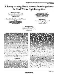
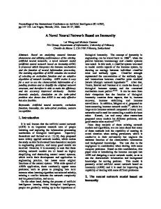
2.2 Web Search Engines Internet assistants have not been practically adopted by Internet users as an interface to reach relevant information; instead Web search engines are preferred option as the portal between users and the Internet due their simplicity. Web search engines are software applications that search for information in the World Wide Web while retrieving data from Web sites and Online databases or Web directories. Web search engines have already crawled the Web, fetched its information and indexed it into databases so when the user types a query, relevant results are retrieved and presented promptly (Fig. 1).
The Internet
Web Crawler
Web Index
Web Search Portal
Web Search Engine
User (Query)
Figure 1: Web search engine architecture The main issues of Web search engines are result overlap, rank relevance and adequate coverage for both sponsored and non-sponsored results as stated by Amanda Spink et al [8]. Web personalization builds user’s interest profile by using their browsing behaviour and the content of the visited Web pages to increase result extraction and rank efficiency in Web search. A model presented by Alessandro Micarelli [9] represents a user needs and its search context is based on content and collaborative personalization, implicit and explicit feedback and contextual search. A user is modelled by Nicolaas Matthijs et al [10] as a set of terms and weights related to a register of clicked URLs with the amount of visits to each, and a set of previous searches and Web results visited; this model is applied to re order the Web search results provided by a non-personalized Web search engine. Web queries are associated by Fang Liu et al [11] to one or more related Web page features and a group of documents is associated with each feature; a document is both associated with the feature and relevant to the query. These double profiles are merged to attribute a Web query with a group of features that define the user’s search relevance; the algorithm then expands the query during the Web search by using the group of categories. Filip Radlinski et al [12] present different methods to improve personalized web search based on the increment of the diversity of the top results where
Page 26 of 246
2 – Web Search personalization comprises the re ranking of the first N search results to the probable order desired by the user and query reformulations are implemented to include variety. The three diversity methods proposed are: the most frequent selects the queries that most frequently precede the user query; the maximum result variety choses queries that have been frequently reformulated but distinct from the already chosen queries, and finally, the most satisfied selects queries that usually are not additionally reformulated but they have a minimum frequency. Spatial variation based on information from Web search engine query records and geolocation methods was included in Web search queries by Lars Backstrom et al [13] to provide results focused on marketing and advertising, geographic information or local news; accurate locations are assigned to the IP addresses that issue the queries. The center of a topic is calculated by the physical areas of the users searching for it where a probabilistic model calculates the greatest probability figure for a geographic center and the geographical dispersion of the query importance. Aspects for a Web query are calculated by Fei Wu et al [14] as an effective tool to explore a general topic in the Web; each aspect is considered as a set of search terms which symbolizes different information requests relevant to the original search query. Aspects are independent to each other while having a high combined coverage, two sources of information are combined to expand the user search terms: query logs and mass collaboration knowledge databases such as Wikipedia.
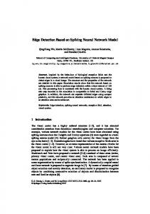
2.3 Metasearch Engines Metasearch engines were developed based on the concept that single Web search engines were not able to crawl and index the entire Web. While Web search engines are useful for finding specific information, like home pages, they may be less effective with a comprehensive search or wide queries due their result overlap and limited coverage area. Metasearch engines try to compensate their disadvantages by sending simultaneously user queries to different Web search engines, databases, Web directories and digital libraries and combining their results into a single ranked list (Fig. 2, Fig. 3). The main operational difference with Web search engines is that Metasearch engines do not index the Web.
Page 27 of 246
2 – Web Search
The Internet
Search Engines (Google – Yahoo – Ask – Bing - Lycos)
Web Directories (Open Directory Project – World Wide Web Virtual Library)
Online Databases (Digital Bibliography & Library ProjectInternational Standard Book Number)
Metasearch Engine (Mamma – Metacrawler – Ixquick – Webcrawler – Dogpile – Vivisimo - Helios)
User (Query)
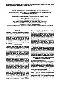
Figure 2: Metasearch services model There are challenges for developing Metasearch engines as described by Weiyi Meng et al [16]: Different Web search engines are expected to provide relevant results which have to be selected and combined. Different parameters were considered by Manoj, M et al [17] when developing a Metasearch engine: functionality, working principles including querying, collection and fusion of results, architecture and underlying technology, growth, evolution and popularity. Numerous metasearch architectures were found by Hossein Jadidoleslamy [18] such as Helios, Tadpole and Treemap with different query dispatcher, result merger and ranking configurations. Helios was presented by Antonio Gulli et al [19]; it is an open source metasearch engine that runs above different Web Search Engines where additional ones can be flexibly plugged into architecture. Helios retrieves, parses, merges, and reorders results given by the independent Web search engines. An extensive modular metasearch engine with automatic search engine discovery was proposed by Zonghuan Wu [20]; it incorporates a numerous number of autonomous search engines is based on three components: “automatic Web search engine recognition, automatic Web search engine interconnection and automatic Web search result retrieval”. The solution crawls and fetches Web pages choosing the Web Search Engine ones, which once discovered, are connected by parsing the HTML source code, extracting the form parameters and attributes and sending the query to be searched. Finally, URLs or snippets provided by the different Web Search Engines are extracted and displayed to the Web user.
Page 28 of 246
2 – Web Search
The Internet
Search Engine
Search Engine
Query Modifier & Dispacher
Merging & Ranking
Meta Search Engine Portal
Meta Search Engine
User (Query)
Figure 3: Metasearch engine architecture There are several rank aggregation metasearch models to combine results in a way that optimizes their relevance position based on the local result ranks, titles, snippets and entire Web Pages. The main aggregation models were defined by Javed A. Aslam et al [21] as: Borda-fuse is founded on the Borda Count, an voting mechanism on which each voter orders a set of Web results; the Web result with the most points wins the election. The Bayes-fuse is built on a Bayesian model of the probability of Web result relevance. The difference between the probability of relevance and irrelevance respectively determines relevance of a Web Page based on the Bayes optimal decision rule. Rank aggregation was designed against spam, search engine commercial interest and coverage by Cynthia Dwork [22]. The use of the titles and associated snippets presented by Yiyao Lu et al [23] produce a higher success than parsing the entire Web pages where the effective algorithm of a metasearch engine for Web result merging outperforms the best individual Web search engine. A formal approach to normalize scores for metasearch by balancing the distributions of scores of the first irrelevant documents was presented by R. Manmatha et al [24], it is achieved by using two different methods: the distribution of scores of all documents and the combination of an exponential and a Gaussian distribution to the ranks of the documents where the developed exponential distribution is used as an approximation of the irrelevant distribution.
Page 29 of 246
2 – Web Search Metasearch engines provide personalized results using different approaches as presented by Leonidas Akritidis et al [25]. The first method provides distinct results for users in separate geographical places where the area information is acquired for the user and Web page server. The second method has a ranking method where the user can stablish the relevance of every Web search engine and adjusts its weight in the result ranking in order to obtain tailored information. The third methods analyses Web domain structures of Web pages to enable the user the possibility to limit the amount of Web pages with close subdomains. Results from different databases present in the Web were also be merged and ranked by Weiyi Meng et al [26] with a database representative that is highly scalable to a large number of databases and representative for all local databases. The method assigns only a reduced but relevant number of databases for each query term where single term queries are assigned the right databases and multi-term queries are examined to extract dependencies between them in order to generate phrases with adjacent terms. Metasearch performance against Web search has been widely studied by B.T. Sampath Kumar et al [27] where the search capabilities of two metasearch engines, Metacrawler and Dogpile, and two Web search engines, Yahoo and Google, are compared.
2.4 Web result clustering Web result clustering groups results into different topics or categories in addition to Web search engines that present a plain list of result to the user where similar topic results are scattered. This feature is valuable in general topic queries because the user gets the theme bigger picture of the created result clusters (Fig. 4). There are two different clustering methods; pre-clustering, as defined by Oren Zamir et al [28], calculates first the proximity between Web pages and then it assigns the labels to the defined groups whereas post-clustering, as proposed by Stanislaw Osinski et al [29], discovers first the cluster labels and then it assigns Web pages to them. Web clustering engines shall provide specific additional features, as established by Claudio Carpineto
et al [30], in
order to be successful: fast subtopic retrieval, topic exploration and reduction of browsing for information. The main challenges of Web clustering are overlapping clusters, shown by Daniel Crabtree et al [31], precise labels as presented by Filippo Geraci [32], undefined cluster number, as experienced by Hua-Jun Zeng et al [33], and computational efficiency.
Page 30 of 246
2 – Web Search
The Internet
Snippets Pre-processing
features extraction
cluster formation
Web cluster Engine User (Query)
Figure 4: Web Cluster Engine Architecture Suffix Tree Clustering (STC) was presented by Oren Zamir et al [28], it is an incremental time method which generates clusters using shared phrases between documents. STC considers a Web page as an ordered sequence of words and uses the proximity between them to identify sets of documents with common phrases between them in order to generate
clusters.
STC
has
three
stages:
document
formatting,
base
clusters
identification and its final combination into clusters. Lingo Algorithm, proposed by Stanislaw Osinski [29], finds first clusters utilizing the Vector Space Model to create a “TxD term document matrix where T is the number of unique terms and D is the number of documents”. A Singular Value Decomposition method is used to discover the relevant matrix orthogonal basis where orthogonal vectors correspond to the cluster labels. Once clusters are defined; documents are assigned to them. A cluster scoring function and selection algorithm, defined by Daniel Crabtree [31], overcomes the overlapping cluster issue; both methods are merged with Suffix Tree Clustering to create a new clustering algorithm called Extended Suffix Tree Clustering (ESTC) which decreases the amount of the clusters and defines the most useful clusters. This cluster scoring function relies on the quantity of different documents in the cluster where the selection algorithm is based on the most effective collection of clusters that have marginal overlay and maximum coverage; this makes the most different clusters where most of the documents are covered in them. A cluster labelling strategy, stablished by Filippo Geraci et al [32], combines intra-cluster and inter-cluster term extraction where snippets are clustered by mapping them into a
Page 31 of 246
2 – Web Search vector space based on the metric k-center assigned with a distance function metric. To achieve an optimum compromise between defining and distinctive labels, prospect terms are selected for each cluster applying a improved model of the information Gain measurement. Cluster labels are defined by Hua-Jun Zeng et al [33] as a supervised salient phrase ranking method based on five properties: “sentence frequency / Inverted document frequency, sentence length, intra cluster document similarity, cluster overlap entropy and sentence independency” where a supervised regression model is used to extract possible cluster labels and human validators are asked to rank them. Cluster diversification is a strategy used in ambiguous or broad topic queries that takes into consideration its contained terms and other associated words with comparable significance. A method proposed by Jiyin He et al [34] clusters the top ranked Web pages and those clusters are ordered following to their importance to the original query however diversification is limited to documents that are assigned to top ranked clusters because potentially they contain a greater number of relevant documents. Tolerance classes approximate concepts in Web pages to enhance the snippets concept vector as defined by Chi Lang Ngo et al [35] where a set of Web pages with similar enhanced terms are clustered together. A technique that learns relevant concepts of similar topics from previous search logs and generates cluster labels was presented by Xuanhui Wang [36], it clusters Web search results based on these as the labels can be better than those calculated from the current terms of search result. Cluster hierarchy groups data over a variety of scales by creating a cluster tree. A hierarchy of snippets, defined by Zhao Li [37], is based on phrases where the snippets are assigned to them; the method extracts all salient phrases to build a document index assigning a cluster per salient phrase; then it merges similar clusters by selecting the phrase with highest number of indexing documents as the new cluster label; finally, it assigns the snippets whose indexing phrases belong to the same cluster where the remaining snippets are assigned to neighbours based on their k-nearest distance. Web search results are automatically grouped through a Semantic, Hierarchical, Online Clustering (SHOC) in Dell Zhang et al [38] experiments; a Web page is considered as a string of characters where a cluster label is defined as a meaningful substring which is both specific and significant. The latent semantic of documents is calculated through the analysis of the associations between terms and Web pages. Terms assigned with the same Web page should be close in semantic space; same as the Web pages assigned with the same terms. Densely allocated terms or Web pages are close to each other in
Page 32 of 246
2 – Web Search semantic space, therefore they should be assigned to the same cluster. Snake is a clustering algorithm developed by Paolo Ferragina et al [39], it is based on two information databases; the anchor text and link database assigns each Web document to the terms contained in the Web document itself and the words included in the anchor text related to every link in the document, the semantic database ranks a group of prospect phrases and choses the most significant ones as labels. Finally, a Hierarchical Organizer combines numerous base clusters into few super clusters. A query clustering approach was presented by Ricardo A. et al [40], it calculates the relevance of Web pages using previous choices from earlier users, the method applies a clustering process where collections of semantically similar queries are identified and the similarity between a couple of queries is provided by the percentage of shared words in the clicked URL within the Web results.
2.5 Travel Services Originally, travel service providers, such as airlines or hotels, used global distribution systems to combine their offered services to travel agencies (Fig. 5). Global distribution systems required high investments due to their technical complexity and physical dimensions as they were mainframe based infrastructure; this generated the monopoly of a few companies that charged a high rate to the travel services providers in order to offer their services to the travel agencies as described by Athina Sismanidou et al [41]. With this traditional model, customers could purchase travel provider services directly at their offices or through a travel agent. This scenario has now been changed by two factors presented by Nelson F. Granados et al [42]: the Internet has enabled ecommerce; the direct accessibility of customers to travel services providers’ information on real time with the availability of online purchase and higher computational servers and software applications can implement the same services as the global distribution systems did, at a lower cost. As a consequence, Hannes Werthner [43] described the new players have entered to this scenario; Software database applications such as ITA Software, or G2 SwitchWorks use high computational server applications and search algorithms to process the data provided from travel services providers; they are the replacement of the global distribution systems.
Page 33 of 246
2 – Web Search
Travel Service Providers (TSP) (Airlines – Hotels – Rental Cars)
Global Distribution Systems (GDS) (Amadeus – Sabre – Galileo – Navitaire - Travelport)
Travel Agencies (TA) (Thomas Cook – Thompson Holidays)
Customer
Figure 5: Traditional travel services model Online travel agents, such as Expedia or TripAdvisor, are traditional travel agents that have automatized the global distribution systems interface; customers can interact with them directly through the Internet and buy the final chosen product. Metasearch engines like Cheapflights or Skyscanner among many others use the Internet to search customers’ travel preferences within travel services providers and online travel agents however customers can not purchase products directly; they are mainly referred to the supplier Web site (Fig. 6). Other players that have an active part in this sector are Google and other Web Search Engines as shown by Bernard J. Jansen et al [44]; they provide search facilities that connect directly travel service providers with consumers bypassing global distribution systems, software distribution systems, Metasearch engines and online travel agents. This allows the direct product purchase that can reduce distribution costs due to a shorter value chain.
Page 34 of 246
2 – Web Search
Travel Service Providers (TSP) (Airlines – Hotels – Rental Cars) Internet Internet Global Distribution Systems (GDS) (Amadeus – Sabre – Galileo Navitaire - Travelport)
Software Database Applications (SDA) (ITA Software – Farologix Triton – G2 SwitchWorks) Internet Internet
On Line Travel Agencies (OTA) (Priceline – Expedia – Orbitz Travelocity – TripAdvisor) Internet Meta Search Engines (MSE) (Cheapflights – kayak – Mobissimo – CheapOair – Skyscanner - Farechase – Travelpack Edreams – Opodo)
Internet
Internet
Internet
Customer
Figure 6: Online travel services model Travel ranking systems, as described by Anindya Ghose et al [45], also recommend products and provide the greatest value for the consumer’s budget with a crucial concept where products that offer a higher benefit are ranked in higher positions. With the integration of the customer and the travel service provider through the Internet, different software applications have been developed to provide extra information or to guide through the purchase process based on user interactions as presented by Zheng Xiang et al [46]. Travel related Web interfaces help users to make the process of planning their trip more entertaining and engaging while influencing users’ perceptions and decisions as described by Bernhard Kruepl et al [47]. There are different information search patterns and strategies proposed by Nicole Mitsche [48] within specific tourism domain web search queries based on search time, IP address, language, city and key terms keywords.
Page 35 of 246
2 – Web Search
2.6 Citation Analysis Citation analysis consists on the access and referral of research information including articles, papers and publications. Its importance is based on its measurement of the value or relevance of personal academic work; it is becoming more respected since its evaluation impacts on other decisions such as promotion, scholarships and research funds. The Journal Impact Factor is calculated by Lokman I. Meho et al [49] as “the number of citations received in the current year to articles published in the two preceding years divided by the total number of articles published in the same two years”. It is based on the concept that high impact journals will only try to publish very relevant work therefore they will be used for outstanding academics. This traditional measurements are peer review based on human judgment however it is time consuming and assessors may be biased by personal judgments such as the quality of journal or the status of university instead of competent and impartial reviews. The Web has provided the possibility of other alternative citation measures making the citation monopoly to change because of the accessibly it provides. New online platforms presented by Judit Bar-Ilan [50] such as Scopus, Web of Science and Google Scholar provide other measures that may represent more accurately the relevance of an academic contribution. Bibliometric indicators proposed by Judit Bar-Ilan [51] evaluate the quality of the publication based on empirical values; mostly number of citations or number of downloads. They are not only quicker to obtain but they also provide a wider coverage because they also retrieve results from relevant academic work published on personal or academic Web pages and open journals based on conference papers, book chapters or thesis. In addition, academics are personally interested to artificially influence ranking methods by “optimizing” the appearance of their research publications to show them in higher ranks with the purpose to extend their reader audience in order to get cited more as exposed by Joeran Beel et al [52]. The h-index defined by Jorge E. Hirsch [53] is applied to qualify the contribution of individual scientific research work; “An academic has an h-index of h if the x publications have individually received at least h citations and the other (x-h) publications have up to h citations”. The h-index has become popular among researchers because it solves the disadvantages of the journal impact factors and it has also a good correlation with the citation analysis database. It is simple and fast to calculate utilizing databases like Google Scholar, Scopus or Web of Science however it suffers some disadvantages [49]; it does not differentiate negative citations from positive ones so both are equally taken into
Page 36 of 246
2 – Web Search account, it does not consider the entire amount of citations an author has collected and it disadvantages a reduced but highly-cited paper set very strongly. Google Scholar is a free Web academic search engine that registers the metadata or the complete text of academic articles from different databases and journals. The result relevance is calculated by a ranking algorithm that combines the term occurrence, author, publications and citations weights following the work of Jöran Beel et al [54]. Google Scholar has received both good and bad critics since it started in 2004 as Dirk Lewandowski [55] stated : The lack of transparency in the relevance assessment of the information due its automatic process of retrieving, indexing and storing information has been criticized; however the more transparent its evaluation algorithms, the easier it becomes to influence its metrics. Google Scholar has been widely analysed and studied by the research community against other online databases by William H. Walters [56] and Anne-Wil Harzing et al [57]. A hybrid recommender system based on
content-based and collaborative-based
relevance was presented by Bela Gipp [58], it expands the method of the traditional keyword or key term search by adding citation examination, author examination, source examination, implicit ratings and explicit marks. Two ranking methods are applied: “intext citation frequency examination” evaluates the occurrence which a publication is “cited within the citing document” and “in-text citation distance examination” determines the similarity between references within a publication by evaluating the word separation.
Page 37 of 246
3 – Ranking
3
Ranking
Ranking is the core process on many information retrieval applications including Web search engines and Recommender systems for two main reasons: the user evaluation of quality or performance from a customer point of view and sponsored adverts based on ranking from a commercial perspective. There are several methods and techniques for ranking Web pages and products that exploit different algorithms built on the analysis of the Web page content, the anchor text of the links between pages or the network structure of the World Wide Web hyperlinked environment.
3.1 Ranking Algorithm Web search engine evaluation comprises the measurement of the quality and services they provider to users; it is also used to compare their different search capabilities. Automatic evaluation analyses the different presented URLs whereas human evaluation is based on the measurement of result relevance; while the latest one is more precise; it takes more effort therefore more expensive as it is normally done by surveys. Other methods that combine both automatic and user evaluation are applications that monitor user activities such as click-troughs or time spent of each Web site. “Dynamic ranking or query-dependent ranking” improves the order of the results returned to the user based on the query while “static ranking or query-independent” calculates the relevance of the Web pages to different topics. There are different methods to assess Web pages relevance. 3.1.1 HTML Properties The first method focuses on the HTML properties of the Web page including the type of text, section, size, position, anchor text and URL. Web spammers base their strategy mostly in the design of the HTML properties of the Web page to get an artificial better ranking from Web search engines. 3.1.2 TF-IDF The second method is founded on the inspection of the Web page text itself and how the words in the query relate within it. TF-IDF or “Term Frequency and Inverse Document Frequency” applies the vector space model with a scoring function where the importance of a term increases if it is repeated often in a document however its weight decreases if the same term appears multiple times on numerous documents as it is considered less descriptive.
Page 38 of 246
3 – Ranking TF-IDF(t,d,D)=TF(t,d)xIDF(t,D)=[1+logft,d ]x [log (1+
N )] dt (1)
where t is the keyword, d is the Web page, ft,d the amount of occurrences that keyword t is contained within the Web page d, N is the entire amount of Web pages and dt is the quantity of Web pages that include the keyword t. A probabilistic TF-IDF retrieval model proposed by Ho Chung Wu et al [59] emulates the decision making of a human brain for two categories of relevance: “local relevance” is first applied to a particular Web page location or section whereas the “wide relevance” spans to cover the whole Web page; the method then merges the “local relevance” decisions for each position as the Web page “wide relevance” decision. Document Transformation adapts the Web page vector close to the query vector by adding or removing terms, an example to long term incremental learning presented by Charles Kemp [60] is based on a search log that stores information about click throughts Web users have browsed among the Web result pages from a Web Search engine and Web Pages selected by the user. Content-Time-based ranking is a Web search time focus ranking algorithm proposed by Peiquan Jin [61] that includes both “text relevance” and “time relevance” of Web pages. “Time relevance” is the interval computed between the query and the content or update time; where every term in a Web page is assigned to an explicit content time interval, finally the time focus TF-IDF value of each keyword is calculated to obtain the overall rank. 3.1.3 Link Analysis The third method is the link analysis which it is founded on the relation between Web pages and their Web graph; Link analysis associates Web pages to neural network nodes and links to neural network edges. In-Degree was defined by Taher H. Haveliwala [62], it was the first link analysis ranking algorithm; it ranks pages according to their popularity which it is calculated by the sum of links that point to the page. Degree(pi )= ∑
pj
pj ∈M(pi )
(2) where p1, p2, … pN correspond to the Web pages to be ranked and M(p i) defines the collection of Web documents pointing to pi.
Page 39 of 246
3 – Ranking Page Rank was proposed by Sergey Brin et al [63], it is founded on the concept that a Web document has a top “Page Rank” if there are many Web pages with reduce “Page Rank” or a few Web pages with elevated “Page Rank” that link to it. Page rank algorithm provides a likelihood distribution that represents the probability that a Web user person arbitrarily following the links will reach to the specific Web page.
PageRank(pi )=
1-d +d ∑ N
PageRank(pj )
pj ∈M(pi )
L(pj ) (3)
where p1, p2, … pN correspond to the Web pages to be ranked, d the dumping factor, M(pi) defines the collection of Web documents pointing to p i, L(pj) is the amount of external connections from page pj and N the entire quantity of Web pages. HITS algorithm or Hyperlink Induced Topic Search algorithm was presented by Jon M. Kleinberg [64], it assigns relevance founded on the authority concept and the relation among a group of relevant “authoritative Web pages for a topic” and the group of “hub Web pages that link to many related authorities” in the Web link arrangement. The hyperlink structure among Web pages is analysed to formulate the notion of authority; the developer of Web document p when inserts a hyperlink to Web document q, provides some relevance or authority on q. Hubs and authorities have a reciprocally strengthening association: “a relevant hub is a Web page that links to many relevant authorities; a relevant authority is a Web page which is linked by numerous relevant hubs”. The authority value of a Web document is the addition of every hub value of Web documents linking to it: n
auth(p)= ∑ hub(i) i=1
(4) where p the relevant authority Web document, i is a Web document linked to p and n is the entire quantity of Web documents linked to p. The hub value of a Web document is the addition of total number of authorities’ values of Web documents linking to it: n
hub(p)= ∑ auth(i) i=1
(5)
Page 40 of 246
3 – Ranking where p is the relevant authority Web document, i is a Web document that p links to and n is the entire quantity of Web documents p connects to. SALSA algorithm or “Stochastic Approach for Link-Structure Analysis” was developed by Ronny Lempel [65], it combines Page Rank and HITS by taking a random walks alternating between hubs and authorities. Two random walks are assigned two scores per Web Page; it is based on the in link and out link that represent the proportion of authority and hub respectively. The hub array is expressed in the below sum: hi,j =
∑ {k|(ih ,ka ),(jh ,ka )∈G}
1 1 x deg(ih ) deg(ka ) (6)
The authority array is expressed in the below sum: ai,j =
∑ {k|(kh ,ia ),(kh ,ja )∈G}
1 1 x deg(ia ) deg(kh ) (7)
where Web document h links to mutually documents i and j and deg is the amount of hyperlinks connecting to a page. QS page-rank is a query-sensitive algorithm proposed by Tao Wen-Xue [66] that combines both global scope and local relevance. Global web Page importance is calculated by using general algorithms such as Page Rank; Local query sensitive relevance is calculated by a voting system that measures the relation between the top Web pages retrieved. The priority of a Query sensitiveness rank (QS) is defined where document 1 is ordered on front of document 2: (QS1> QS2) || (QS1 == QS2 && PR1> PR2) (8) The priority of a Global importance rank (PR) is defined where document 1 is ordered on front of document 2: (PR1> PR2) || (PR1 == PR2 && QS1> QS2) (9) where QS1 and QS2 are the Query sensitive values and PR1 and PR2 are the Global importance values for document 1 and document 2 respectively.
Page 41 of 246
3 – Ranking
DistanceRank was defined by Ali Mohammad Zareh Bidoki [67], it is an iterative algorithm built on reinforcement learning; distance between pages is counted as punishment where distance is established as the amount of links among two Web Pages. The objective of the method is the reduction of the punishment or distance therefore a Web document with reduced “distance” has a greater rank. The main concept is that as correlated Web pages are connected between them; the distanced built method finds relevant Web pages quicker. distancen[j]=(1-α)·distancen-1[j] + α·mini(log(O[i])+distancen-1[i]) (10) where i is the collection of Web documents linking to j and O[i] is the amount of outbound hyperlinks in Web document i and α is the learning rate of the user. DING is a Dataset Ranking algorithm presented by Renaud Delbru [68] that calculates dataset ranks; it uses the connections among them to combine the resulting scores with internal semantic based ranking strategies. DING ranks in three stages: first, a dataset rank is calculated by an external dataset hyperlink measurement on the higher layer, then for each dataset, local ranks are calculated with hyperlink measurements between the inner entities and finally the relevance of each dataset entity is the combination of both external and internal ranks. The internal rank score of entity e is calculated as: r(e)=wσ,i,j =LF(Lσ,i,j )xIDF(σ)=
|Lσ,i,j | ∑Lr,i,k|Lr,i,k |
xlog
N 1+frequency(σ) (11)
where Lσ,i,j is a linkset (σ is term, i is the source and j is the target), N represents the amount of datasets and freq(σ) defines the rate of appearance of the term σ in the group of datasets. The dataset rank score is calculated as: rk (Dj )=α ∑ rk-1 (Di )wσ,i,j +(1-α) Lσ,i,j
|EDj | ∑D∈G|ED | (12)
where D is a dataset and EDj is the set of nodes within Dj
Page 42 of 246
3 – Ranking The final global score of entity e for dataset D is: rg(e) = r(e)·r(D) (13) where r(e) and r(D) are the internal rank entities and dataset rank score respectively ExpertRank was proposed by Jian Jiao [69], it is an online community and discussion group expert ranking algorithm that integrates a vector space method to calculate the expert subject importance and a method similar to Page Rank algorithm to evaluate topic authority. Expert subject relevance score is calculated as a likeness of the candidate description and the provided request where the candidate description is generated by combining all the comments in the topic conversation group and the authority rating is computed according to the user interaction graph. Expert(c,q)=i(RE(c,q),AU(c)) (14) where c is the candidate, q is the query, i is the integration method, RE(c,q) represents the relevance rating among the query q and candidate ca’s knowledge and AU(c) represents the authority rating.
3.2 Relevance Metrics Performance can be described as the display of relevant, authoritative, updated results on first positions. Retrieval performance is mostly evaluated on two parameters: precision is the percentage of applicable results within the provided Web document list and recall is the percentage of the entire applicable results covered within the provided Web document list. Due the intrinsic extent of the Web, where it is difficult to measure the quantity of all Web pages and the fact users only browse within the first 20 results; precision is widely used as a performance measurement. In addition, another factor to consider is that Web search engines are different and therefore they perform differently as exposed by Mildrid Ljosland [70]; some may perform better than others for different queries and metrics. There are different parameters to assess the performance of recommender systems: -
Precision evaluates the applicability of the first N results of the rating result set in relation to a query:
Page 43 of 246
3 – Ranking
P@N=
Number of relevant documents in top N results N (15)
-
Recall represents the applicability of the first N results of the rating result set in relation to the complete result set:
R@N=
Number of relevant documents in top N results S (16)
where S is the result set. -
The Mean Absolute Error (MAE) evaluates the error between user predictions and user ratings: MAE=
∑N d=1|Pui -Rui | N (17)
-
The Root Squared Mean Error (RSME) measures the differences between predictions and user ratings:
RME=
2 √∑N d=1(Pui -Rui )
N (18)
where Pui is the forecasted ranking for u on product i, R ui is the current rank for u on product i and N the entire amount of products ranked by the user u. -
F-score combines Precision and Recall in an evenly weighted metric:
Fmeasure =
2*Precision*Recall Precision+Recall (19)
-
The Average Precision calculates the mean figures of P@n over the number n of retrieved Web pages:
AP=
∑N n=1 P@n*rel(n) Number of relevant documents for this query (20)
Page 44 of 246
3 – Ranking where N is the total amount of retrieved Web pages in the result list, and rel(n) represents that the n-th Web page is either applicable or not to the query with values 1 or 0. -
The Mean Average Precision measures the balance of average precision within a collection of Q Web searches:
MAP=
∑Q q=1 AP(q) Q (21)
-
The Normalized Discounted Cumulative Gain uses a rated relevance metric to measure the relevance of a result that uses its rank within the Web page set: N
NDCG@N=ZN ∑ j=1
R(j)
2 -1 log2 (1+j) (22)
where R(j) is the rated applicability of the result at position j within the Web page set, ZN is the standardization parameter that assures the optimum NDDC@N matches to 1. For binary ranking then R(j) is fixed to 1 when the result at position j is relevant to the Web search and is fixed to 0 when the Web page is irrelevant. -
TREC average precision includes rank position on the performance evaluation; it is defined at a cutoff N:
TSAP@N=
∑N i=1 ri N
{
ri = 1⁄i if the ith ranked result is relevant
ri =0 if the ith ranked result is not relevant or duplicate
} (23)
-
The Reciprocal Rank of a Web search is defined as the multiplicative inverse applied to the rank of the first relevant result: RR=
1 ranki (24)
where ranki is the order of the first relevant result. -
The Mean Reciprocal Rank corresponds to averaged value of the RR (Reciprocal Rank) over a collection of Q searches:
Page 45 of 246
3 – Ranking MRR=
∑Q q=1 RR(q) Q (25)
where RR(q) is the Reciprocal Rank associated to the search q and Q is the total collection of searches. -
The Expected Reciprocal Rank is based on a cascaded model which penalizes documents which are shown below very relevant documents: N
r-1
r=1
i=1
1 ERR= ∑ ∏(1-Ri )∙Rr r (26) where N is the amount of Web pages in the ranking, r is the position at which the Web user stops its search, R measures the probability of a click which can be interpreted as the relevance of the snippet. Different research analyses have studied the efficiency of Web search engines by Michael D. Gordon et al [71] and the level of overlap among the Web pages presented by the search engines. Two new measurements to assess Web search engine performance are proposed by Liwen Vaughan [72]: the relevance of result rating by a Web search engine is assessed by the association among Web and human rating and the capability to retrieve applicable Web pages as the percentage of first ranked within the retrieved Web pages. Four relevance metrics are applied by Longzhuang Li [73] to calculate the quality of Web search engines; three of them are adapted from the Information Retrieval: Vector Space method, Okapi likeness value and Coverage concentration rating and a new method which is developed from the human interaction to take human expectations into account based on a raw score and a similarity score. The Text REtrieval Conference (TREC), as presented by Amit Singhal et al [74], is supported by the “National Institute of Standards and Technology (NIST)” and “U.S. Department of Defence” to sponsor studies in the information and data retrieval research group; TREC provides the framework for extensive evaluation applied to different text retrieval methods. Effectiveness of TREC algorithms against Web search engines has been compared by Amit Singhal et al [74] where tested algorithms were developed with Okapi or Smart based on the term weighting methods (TF-IDF). Web search engines are evaluated against a series of relevance metrics by David Hawking et al [75] and [76]: precision, TREC based mean reciprocal rank (MRR) and the TREC style average precision
Page 46 of 246
3 – Ranking (TSAP) obtained from double relevance human evaluations for the top 20 Web results displayed. Web search evaluation methods was be assigned into eight different categories by Rashid Ali et al [77]: assessment founded on relevance, assessment founded on ranking, assessment founded on user satisfaction, assessment founded on size and coverage of the Web, assessment founded on dynamics of Search results, assessment founded on few relevant and known items, assessment based on specific topic or domain and automatic assessment. Different Automatic Web search engine evaluation methods have been proposed by Fazli Can et al [78] and Rashid Ali et al [79] to reduce human intervention. The algorithm first submits a query to the different Web search engines where the top 200 Web pages of every Web search engine are retrieved; then it ranks the pages in relation to their likeness to the Web user information requirements; the model is built on the vector space method for query-document matching and ranking using TF-IDF. After ranking; the method lists as relevant the Web pages that are in the first 20 documents retrieved by each Web search engine with the top 50 ranked results. An automatic C++ application presented by Jinbiao Hou [80] compares and analyses Web result sets of several Web search engines; the research analyses the URL coverage and the URL rank where recall and accuracy are used as relevance metrics however there is not description regarding the method that decides URL relevance. A technique for evaluating Web search engines robotically presented by Abdur Chowdhury et al [81] is founded in the way they order already rated Web search results where a search query is transmitted to different Web search engines and the rank of retrieved Web results from is measured against the document that has already been paired with that query. Web search engine evaluation has been examined from a webometric perspective by Mike Thelwall [82] using estimates of success values, amount of provided URL, amount of domains retrieved and number of sites returned where evaluations are made to assess the retrieval of the most precise and comprehensive Web results from every single Web engine.
Page 47 of 246
3 – Ranking
3.3 Learning to Rank Learning to rank is defined as the implementation of semi-supervised or supervised computer learning techniques to generate a ranking model by combining different documents features obtained from training data in an information retrieval system. The training data contains sets of elements with a specified position represented by a numerical score, order or a binary judgment for each element. The purpose of a ranking method is to order new result lists in order to produce rankings similar to the order in the training data. Query document sets are normally defined by quantitative vectors which components are denoted features, factors or ranking signals. The main disadvantages of the learning to rank approach are that the optimization of relevance is based on evaluation measurements without addressing the decision of which measures to use; in addition, learning to rank does not take into consideration that user relevance judgment changes over the time. The model of learning to rank consists on: -
a set Q of M queries, Q = {q1, q2, ..., qM}
-
a set D of N Web pages per query qM, D = { d11, d12, ..., dNM}
-
a set X of M feature vectors per each query q M and Web page dN pairs, X = {x11, x12, ..., xNM}
-
a set Y of M relevance decisions per each query q M and Web page dN pairs, Y = {y11, y12, ..., yNM}
The set of query-Web page pairs {qM, dNM} has associated a set of feature vectors {xNM} that represents specific ranking parameters describing the match between them. The set of relevance judgments {yNM} can be a binary decision, order or score. Each feature x NM and the corresponding score yNM form an instance. The input to the learning algorithm is the set feature vectors {xNM} that represents the pair {qM, dNM} and the desired output corresponds to set of relevance judgement {yNM}. The ranking function f(x) is acquired by the learning method during the training process on which relevance assessments are optimized with the performance measurement or cost function (Fig. 7).
Page 48 of 246
3 – Ranking
(q1 , d11) (q1 , d21) (q1 , dN1)
Feature extractor
(qM , d1M) (qM , d2M) (qM , dNM)
Relevance judgement
Training set
Instances {xNM , yNM}
Ranking function f(x) Cost function Learning algorithm
y1M=f(qM , d1M) y2M=f(qM , d2M) yNM=f(qM , dNM) Ordered results
(q1 , d11) (q1 , d21) (q1 , dN1) (qM , d1M) (qM , d2M) (qM , dNM) Test set
Ranking system
Figure 7: Learning to Rank Model RankSVM learning to rank algorithm learns retrieval functions using clickthrough data for training based on a Support Vector Machine (SVM) approach as presented by Thorsten Joachims [83]. It uses a mapping function to correlate a search query with the features of each of the possible results where each data pair is projected into a feature space combined with the corresponding click-through data that measures relevance. Distinct ranking methods are developed for several classes of contexts by Biao Xiang et al [84] based on RankSVM that integrates the ranking principles into a new ranking model that encodes the context details as features. It learns a Support Vector Machine model for a binary categorization on the selection between a couple of Web pages where the evaluation is based on human conclusions and indirect user click. A machine learned ranking model defined by Anlei Dong et al [85] routinely perceives and reacts to recent related queries where recent ranking takes into account freshness and relevance; the system is divided into two approaches: a high accuracy recent related query detector and a specific recent related sorter trained to represent the characteristics and data distribution applicable for recent ordering. Random Forests is a low computational cost alternative to point-wise ranking approach algorithm presented by Ananth Mohan [86], it is founded on the machine learning method “Gradient Boosted Regression Trees”. The learning algorithm of Random Forests is applied multiple times to different subsets and the results are averaged whereas Gradient Boosted Regression Trees sequentially adds small trees at each iteration instead of training many full trees. The combination of both two algorithms first learns a ranking function with Random Forests and later uses it as initialization for Gradient Boosted Regression Trees.
Page 49 of 246
4 – Recommender Systems
4
Recommender Systems
Recommender systems predict users’ interest of different items or products providing a set of suggested items applying tailored relevance algorithms. Recommender systems consist on a database where user ratings and item description are stored and updated iteratively. A user interface interacts with the user where a profiler extracts user properties with explicit and implicit feedback; different suggestions and their order are computed by the recommender ranking algorithm (Fig. 8). Due their filtering properties they are widely used within e-commerce as presented by Lee Wei-Po et al [87] because they also support e-commerce customers to find rare products they might not have discovered by themselves.
Items Item – User Database
Recommender Algorithm
Profiler
Web Portal
User
Users Recommender System
Figure 8: Recommender system architecture
4.1 Recommender System Types There are two main different categories of recommender systems (Fig. 9) as described by Dhoha Almazro et al [88]. Content-based recommender systems are built on a description of the product and a profile of the customer’s wishes where different properties of the items and users are used to identify products with similar features without including other user’s ratings. They suffer from some disadvantages as presented by Gediminas Adomavicius et al [89] such as its inability to recommend completely different items that the user may also consider relevant and a customer needs to mark several products before getting relevant recommendations. Collaborative recommender systems are founded on the customer’s previous marks to other products and the consideration of other decisions made by similar users; they made suggestions based on a high correlation between users or items. Although collaborative recommendation reduces the issues from the Content-based solution; it has other drawbacks such as it needs a large number of rating data to calculate accurate correlations and predictions; it also ignores on its calculations new added users or items. Hybrid Recommender Systems take a combination of both approaches.
Page 50 of 246
4 – Recommender Systems
Single User
Content Based
Multi User User Based
Item Based
Collaborative
Recommender System
Figure 9: Common types of Recommender systems In a multi-criteria ranking recommenders, users give ratings on several characteristics of an item as a vector of ratings as defined by Gediminas Adomavicius et al [90] whereas cross domain recommender systems suggest items from multiple sources with item or user based formulas founded on locality collaborative filtering as presented by Paolo Cremonesi et al [91]; they operate by first modelling the traditional likeness association as a directly connected graph and then exploring the entire potential paths that links users or items to discover new cross domain associations. There are several relevance metrics for assessment of recommender systems in various e-commerce business frameworks presented by Gunnar Schröder et al [92]; accuracy evaluation metrics are allocated into three major categories: predictive based on the error between estimated and true user ratings, classification based on the successful decision making and rank based on the correct order. Social network information is inserted to recommender systems by Xiwang Yang et al [93] as an additional input to improve accuracy; Collaborative Filtering based social recommender systems are classified into two categories: matrix factorization approach where user to user social information is integrated with user item feedback history and neighbourhood based social approaches based on social network graphs.
4.2 Recommender System Relevance Metrics The user based recommender generally uses the Pearson’s relationship similarity: similarity(u,v)=
∑i∈M(ru,i -r̅u ) ∗ (rv,i -r̅v ) √∑i∈M(ru,i -r̅u )2 ∗ √∑i∈M(rv,i -r̅v )2 (1)
which the prediction on the user-based is defined below:
Page 51 of 246
4 – Recommender Systems prediction (u,i) = r̅u +
∑v∈N(u) similarity(u,v) ∗ (rv,i -r̅v ) ∑v∈N(u)|similarity(u,v)| (2)
where N(u) defines a set of neighbours of u, similarity(u,v) represents the correlation between user u and v, ru,i is the mark of customer u to product i, 𝑟̅𝑢 is the average rating of customer u and M is the total quantity of items. The item based recommender systems generally use the Cosine Similarity: similarity(u,v)=
∑N d=1 id *pd 2 N 2 √ ∑N d=1 id *√∑d=1 pd
(3) although the Euclidean distance similarity can also be used: N
similarity(i,p) = √ ∑(id -pd )
2
d=1
(4) and the Manhattan distance similarity: N
similarity(i,p) = ∑|id -pd | d=1
(5) which the prediction on the item-based is defined below: prediction (u,i) =
∑q∈N(i) similarity(i,q)*ru,q ∑q∈N(i) similarity(i,q) (6)
where N(i) is a collection of neighbours of i and similarity(i,p) is the correlation between item i and p, id the relevance of item i to user d and N the overall quantity of users. The linear prediction on the content-based is defined below: N+M
prediction(u,i)=〈w,x〉= ∑ wq xq q=1
(7) where x are the instance vectors and w the matrix weights.
Page 52 of 246
4 – Recommender Systems
4.3 Recommender System Model The model of a Recommender system (Fig. 10) consists on: -
A set Q of N users, Q = {u1, u2, ..., uN}
-
A set I of M items, I = { i1, i2, ..., iM}
-
A rating matrix R, R=[rij] where i ∈ Q and j ∈ I
-
A set X of N feature vectors, X = {x1, x2, ..., xN}
-
A weight matrix W, W=[wij] where i ∈ N and j ∈ N+M
r11 r12 r21 r22 r31 r32 rN1 rN2 {i1,i2,i3,iM}
r13 r1M r23 r2M r33 r3M rN3 rNM
Rating Matrix
sim(u1,uN) sim (i1,iM)
Similarity
Item Set {u1,u2,u3,uN} User Set
Collaborative-user Collaborative-item Recommender type
pred(u,i)
Content-based
Prediction
{(x1 = u1, i1, iM), (x2 = u2, i1, iM), (x3 = u3, i1, iM), (xN = uN, i1, iM)}
w1 = w11,w12,w1M w2 = w21,w22,w2M w3 = w31,w32,w3M wN = wN1,wN2,wNM
Feature Set
Weights
Figure 10: Recommender system model The set of user-items {uN, iM} has an associated set of feature vector {xN} that represents users and the different items assigned to them in the Content model. The relevance judgement pred(u,i) can be a binary decision, order or score based on the similarity between users or items in the Collaborative model and weights in the Content model.
Page 53 of 246
5 – The Random Neural Network
5
The Random Neural Network
5.1 Neural Networks Artificial neural networks are models inspired by the brain central nervous system. They are usually presented as artificial nodes or "neurons" in the different layers connected together via synapses to form a network which mimics a biological neural network. The synapses have values called "weights" which value is updated during network calculations. There are two main models to represent a neural network (Fig. 11); the feed forward model where connections between the neurons follow only the forward direction and the recurrent model where connections between neurons form a direct cycle. Recurrent Model
Feed Forward Model
4 1 1
5
2
6
3
7
9
2
3
4
Input / Output Nodes
10
8
Input Nodes
Hidden Nodes
Output Nodes
Figure 11: Artificial Neural Network – Recurrent and feed forward models Artificial neural networks are normally defined by three parameters: the interconnection layout between different layers of neurons; the learning process for updating the weights of the interconnections and the activation function that converts a neuron's weighted input to its output activation.
Page 54 of 246
5 – The Random Neural Network Artificial neural networks have been used to solve a wide variety of tasks that would have been difficult to resolve by ordinary rules based programming, including computer vision speech and pattern recognition. The learning capabilities of neural networks are the properties that have attracted the most interest; learning uses a set of observations to find which network weighs solve a specific task in some optimal sense. The cost function is an important concept in learning, as it measures how far away a particular solution is from an optimal solution. There are three major learning methods: supervised learning, unsupervised learning and Reinforcement Learning. Supervised learning finds a function, f, that from a given input - output pair (x, y) matches them. The cost function, C, is related to the mismatch between the artificial neural network approximation, f(x) and the output, y. A commonly used cost is the mean-squared error, which tries to minimize the average squared error between the network's output, f(x), and the target value y over the example pair. An input x is given in unsupervised learning and the cost function, C, to be minimized depends on the task that it is tried to be modelled and priori assumptions like implicit properties of the model, its parameters or the observed variables. The input x is usually not given in Reinforcement Learning; it is generated by an agent's interactions with the environment. At each point in time t, the agent performs an action and the environment generates an observation and an instantaneous cost C, according to some dynamics. The aim is to discover a rule for selecting actions that minimizes some long-term cost.
5.2 Deep Learning Deep Learning models high level abstractions in data by using a network with multiple processing layers, composed of multiple linear and non-linear transformations. Deep learning is a branch of machine learning based on modelling representations of data. Deep learning is characterized as using a cascade of l-layers of non-linear processing units for feature extraction and transformation (Fig. 12); each successive layer uses the output from the previous layer as input. Deep learning learns multiple layers of
Page 55 of 246
5 – The Random Neural Network representations that correspond to different levels of abstractions; those levels form a hierarchy of concepts where the higher the level, the more abstract concepts are learned.
Deep Learning Model
b1
k1
l1
a1
b2
k2
l2
ak
b3
k3
l3
ax
bk
kk
lk
by
kz
lw
Layer 1
Layer k
Layer l
Input Nodes
nk
nv
Output Nodes
Hidden Nodes
Figure 12: Artificial Neural Network – Deep Learning model There
are
various
deep
learning
architectures
such
as
deep
neural
networks,
convolutional deep neural networks, deep belief networks and recurrent neural networks. This research is based on a deep neural network which is an artificial neural network with multiple hidden layers of units between the input and the output layers. Deep learning suffers two major issues; they do not generalize well due the additional layers of abstraction and they have a major computational learning time.
5.3 G-Networks G-Networks or Gelenbe Network was presented by Erol Gelenbe [121] and Erol Gelenbe et al [122], it is a model for neural networks as well as queueing systems with specific control functions, such as traffic routing or destruction. A product form solution to Jackson's theorem, but which requires the solution of a system of non-linear equations for the traffic flows as presented by Erol Gelenbe [123], exists for the stationary distribution of G-networks as demonstrated by Erol Gelenbe et al [124].
Page 56 of 246
5 – The Random Neural Network A G-Network is an open network of G-queues with several types of customers: -
positive customers arrive from other queues or arrive externally as Poisson arrivals, and conform to normal service and routing rules as in conventional network models [123];
-
negative customers arrive from another queue, or which arrive externally as Poisson
arrivals,
and
remove
customers
in
a
non-empty
queue
[123],
representing the need to remove traffic when the network is congested, including the removal of "batches" of customers [125]; -
"triggers" arrive from other queues or from outside the network and they displace customers and move them to other queues [126];
-
"resets" arrive from other queues or from outside the network and they set the empty queue to a random length whose distribution is identical to the stationary distribution at that queue [127,128]. A reset which arrives to a non-empty queue has no effect.
The G-queues that forms the G-network must have the following properties: -
each G-queue has one server, that serves at rate μ(i);
-
external arrivals of positive customers or of triggers or resets form Poisson processes of rate Λ(i), for positive customers, while triggers and resets, including negative customers, form a Poisson process of rate λ(i);
-
a positive customer acts as usual when it arrives to a queue and increases the queue length by 1;
-
a negative customer reduces the length of the queue by some random number (if there is at least one positive customer present at the queue) when it arrives to a queue. A trigger moves a customer probabilistically to another queue and a reset sets the state of the queue to its steady-state if the queue is empty when the reset arrives. Triggers, negative customers and resets disappear after they have taken their action;
-
a customer moves from queue i to queue j when a service is completed as a positive customer with probability p+(i,j) as a trigger or reset with probability p(i,j) and departs the network with probability d(i).
G- Networks were extended to of multiple classes of positive and negative customers by Jean-Michel Fourneau et al [129] and Erol Gelenbe et al [130]. A positive customer class is characterized by the routing probabilities and the service rate parameter at each
Page 57 of 246
5 – The Random Neural Network service center while negative customers of different classes may have different "customer destruction" capabilities. G-networks have been used in a wide range of applications by Erol Gelenbe [131,132], such as single server presented by Erol Gelenbe et al [133] and resource allocation in multimedia systems as proposed by Erol Gelenbe et al [134].
5.4 The Random Neural Network The Random Neural Network was presented by Erol Gelenbe [135]; it is a spiked recurrent stochastic model. The main analytical properties are the “product form” and the existence of an unique network steady state solution. The Random Neural Network model represents more closely how signals are transmitted in many biological neural networks where they travel as spikes rather than as fixed analogue signals. 5.4.1 Principles The Random Neural Network consists on n-neurons (Fig. 13). The state of the n neuron network at time t is represented by the vector of non-negative integers k(t) = [k1(t), … ki(t)] where ki(t) is the potential of neuron i at time t. Neurons interact with each other by interchanging signals in the form of spikes of unit amplitude: -
A positive spike is interpreted as excitation signal because it increases by one unit the potential of the receiving neuron;
-
A negative spike is interpreted as inhibition signal decreasing by one unit the potential of the receiving neuron or has no effect if the potential is already zero.
Each neuron accumulates signals and it will fire if its potential is positive. Firing will occur at random and spikes will be sent out at rate r(i) with independent, identically and exponentially distributed inter-spike intervals: -
Positive spikes will go out to neuron j with probability p+(i,j) as excitatory signals;
-
Negative spikes with probability p-(i,j) as inhibitory signals.
Page 58 of 246
5 – The Random Neural Network
Positive signals Negative signals Neuron State
Neuron Fires
Excitation Inhibition Potential – Non Negative Excitation signal arrives Inhibition signal arrives
Increases +1 Decreases -1
Only if Potential is positive Emission of Excitation Spike Emission of Inhibition Spike
Decrease potential -1 Decrease potential -1
Figure 13: Random Neural Network: Principles
5.4.2 Model A neuron may send spikes out of the network with probability d(i). We have: n
d(i)+ ∑[p+ (i,j)+p- (i,j)]=1
for 1 ≤ i ≤ n
j=1
(1) Neuron potential decreases by one unit when the neuron fires either an excitatory spike or an inhibitory spike (Fig. 14). External (or exogenous) excitatory or inhibitory signals to neuron i will arrive at rates Λ(i), λ(i) respectively by stationary Poisson processes. The Random Neural Network weight parameters w +(j,i) and w-(j,i) are the non-negative rate of excitatory and inhibitory spike emission respectively from neuron i to neuron j: -
w+(j,i) = r(i)p+(i,j) ≥ 0;
-
w-(j,i) = r(i)p-(i,j) ≥ 0. (2)
Information in this model is transmitted by the rate or frequency at which spikes travel. Each neuron i, if it is excited, behaves as a frequency modulator emitting spikes at rate w(i,j) = w+(i,j) + w-(i,j) to neuron j. Spikes will be emitted at exponentially distributed random intervals. Each neuron acts as a non-linear frequency demodulator transforming the incoming excitatory and inhibitory spikes into potential. This network model has a product form solution; the network’s stationary probability distribution can be represented as the product of the marginal probabilities of the state of each neuron as demonstrated by Erol Gelenbe [136].
Page 59 of 246
5 – The Random Neural Network
Λi : Arrival rate of external excitatory signal Λi q1r1(p
+
λi : Arrival rate of external inhibitory signal
-
+
1,i+p 1,i)
qiri(p qi
i,1+p i,1)
qi : Probability neuron excited
di
qkrk(p+k,i+p-k,i)
ri : Rate neuron fires spikes
qiri(p+i,k+p-i,k)
p+: Probability excitatory signal neuron i -> neuron j p-: Probability inhibitory signal neuron i -> neuron j
λi
di: Probability signal leaves network w+j,i = rip+i,j w-j,i = rip-i,j
Non negative rates spike emission Excitatory / Inhibitory
n
[p+i,j + p-i,j ] = 1
di + j=1
Figure 14: Random Neural Network: Model 5.4.3 Theorem Let’s define the probability distribution of the network state as p(k,t) = Prob[k(t) = k)] and the marginal probability a neuron i is excited at time t as qi(t) = Prob[ki(t)>0] (Fig. 15). The stationary probability distribution p(k) = lim t∞p(k,t) and qi = limt∞qi(t) where k(t) is a continuous time Markov chain that satisfies Chapman-Kolmogorov equations. Let’s define: n
+
λ (i) qi = r(i)+λ (i)
r(i)= ∑[w+ (i,j)+w- (i,j)]
for 1 ≤i ≤n
j=1
(3) +
-
where the λ (i), λ (i) for i=1,…,n satisfy the system of nonlinear simultaneous equations: n + λ (i)= ∑ [qj r(j)p+ (j,i)] +Λ(i) j=1 n λ (i)= ∑ [qj r(j)p- (j,i)] +λ(i) j=1
(4) +
-
If a nonnegative solution {λ (i),λ (i)} exists to the equations 1 and 2 that meets q i < 1 then: n
p(k)= ∏[1-qi ]qki i i=1
(5) The network will be stable if a value q i < 1 can be found. The average potential at a neuron i is qi/[1-qi] and the rate of emission of spikes from neuron i in steady state is
Page 60 of 246
5 – The Random Neural Network qir(i). If we have λ+(i) > [r(i) + λ-(i)] for any neuron means that the neuron is unstable or saturated; this implies that it is constantly excited in steady state and its rate of excitatory and inhibitory spike emission r(i) to another neuron j will be r(i)p +(i,j) and r(i)p-(i,j) respectively.
k(t) = [k1(t), … , kn(t)] k = (k1, … , kn) p(k) = limt->∞ Prob[k(t)=k]
Vector State / Potential n neuron time t Particular value vector Stationary Probability Distribution Method A
Method B
n
qi =
λi+ = Λi +
Ni
λi+
Di
ri + λi-
0 < qi < 1
i = 1, …,n
qjw+j,i j=1 n
λi- = λi +
qjw-j,i j=1
Fi =
ri ri + λi-
n
p(k) =
[1-qi]qiki
i=1
λi+ = Λi (I-Fip+i,j)-1 λi- = λi+Fip-i,j + λi
n
w+i,j+w-i,j
ri = j=1
Figure 15: Random Neural Network: Theorem
5.4.4 Learning Algorithm: Gradient Descent Neural networks are capable to learn iteratively through examples or training sets. The two main methods are supervised learning based on an input with the desired output and Reinforcement Learning based on the environment reactions from user actions. The Random Neural Network learning algorithm proposed by Erol Gelenbe [137] is based on gradient descent of a quadratic error function (Fig. 16). The backpropagation model requires the solution of n linear and n nonlinear equations each time the n neuron network learns a new input and output pair. Gradient Descent learning algorithm optimizes the network weight parameters w in order to learn a set of k input-output pairs (i,y) where successive inputs are denoted i = {i1,…,ik} and the successive desired outputs are represented y = {y1,…,yk}. Each input vector ik = (Λk, λk) is the pair of the excitatory and inhibitory signals entering each neuron: ΛK = [ΛK(1),…, ΛK(n)], λK = [λK(1),…, λK(n)]. Each output vector yK = (y1k,…, ynk), yik Є [0,1] is composed the desired values of each neuron. The desired output vectors are approximated by minimizing the cost function Ek:
Page 61 of 246
5 – The Random Neural Network n
1 2 Ek = ∑ ai (qi -yik ) 2
ai ≥0
i=1
(6) Each of the n neurons of the network is considered as an output neuron. The function of the variable ai is to remove neurons from the network output. The network learns both n x n weight matrices Wk+={wk+(i,j)} and Wk-={wk-(i,j)} by calculating new values of the network parameters for each input i k = (Λk, λk) using Gradient Descent. The rule for weight update can take the generic form: n
wk (u,v)=wk-1 (u,v)-η ∑ ai (qik -yik ) [ i=1
∂qi ] ∂w(u,v) k (7) +
-
where η is the learning rate and the term w(u,v) denotes either w (u,v) or w (u,v) To evaluate the partial derivatives we define the vector q = (q 1,…,qn) and the n x n matrix: W=
w+ (i,j)-w- (i,j)qj -
r(i)+λ (i)
for i,j = 1,…, n (8)
We also define the n-vectors: γ+(u,v) = [γ1+(u,v),…, γn+(u,v)] (9) and γ-(u,v) = [γ1-(u,v),…, γn-(u,v)] (10) where:
-1 if u=i,v≠i r(i)+λ (i) +1 (u,v)= γ+ i if u≠i,v=i r(i)+λ (i) {0 for all other values of (u,v)}
-(1+qi ) if u=i,v=i r(i)+λ (i) -1 γ-i (u,v)= if u=i,v≠i r(i)+λ (i) -qi if u≠i,v=i r(i)+λ (i) {0 for all other values of (u,v)}
The vector equations can be written: ∂q ∂q = W+γ+ (u,v)qu ∂w+ (u,v) ∂w+ (u,v)
Page 62 of 246
5 – The Random Neural Network ∂q ∂w- (u,v)
=
∂q ∂w- (u,v)
W+γ- (u,v)qu
or equivalently: ∂q ∂w+ (u,v)
=γ+ (u,v)qu [I-W]-1
∂q =γ- (u,v)qu [I-W]-1 ∂w- (u,v) (11) where I denotes the n x n identity matrix.
(ik,Yk)
Input – Desired Output Pairs Input
ik = {[Λk(1), ... , Λk(n)] , [λk(1), ... , λk(n)]}
Output
yk = {[y11 , ... , y1k] , [yn1 , ... , ynk])
Λk , λk , ynk Є [0,1] Ek = Wk
n
1
Ek = Cost function to minimize
ai(qi – yik)2
2
ai = output neurons
i=1
Wk =
{Wk+,Wk-}
=
{wk+i,j
, wk-i,j}
n
wk (u,v) = wk-1(u,v) - η
ai(qik – yik) i=1
dqi dw+(u,v)
dw(u,v)
=ψi+(u,v)qu[I-W]-1
ψi+(u,v)
=ψi-(u,v)qu[I-W]-1
ψi-(u,v)
k
dqi dw-(u,v)
dqi
k
η: learning rate k = -1/Di (u=i , v≠i) = +1/Di (u≠i , v=i) = 0 rest (u,v) = -1/Di (u=i , v≠i) = -qi/Di (u≠i , v=i)
W=
w+i,j -qjw-i,j ri + λi-
-(1+qi)/Di (u=i , v=i) 0 rest (u,v) Di = ri + λi-
Figure 16: Random Neural Network: Gradient Descent learning The complete learning algorithm can be specified. We need first to appropriately initiate the weight matrices W0+ and W0- (Fig. 17). The network weight initialization method is based on the random initialization. A value for η needs to be selected and for each successive value of k: 1- Set the input values to ik = (Λk, λk). 2- Solve the system of non-linear equations 3 and 4. 3- Solve the linear equations 11 with the results of 4. 4- Update the weight matrices Wk+ and Wk- following the equation 4 using the results of 4 and 6. 5- Evaluate the cost function Ek according to equation 6 using the results of 7.
Page 63 of 246
5 – The Random Neural Network
We iterate this learning algorithm until the value of the cost function from the network weight matrices is smaller than some predetermined value.
Initialize Random Values Wk = {Wk+,Wk-}
Set Input / Desired output (ik,Yk)
Solve linear equations dqi dqi dw+(u,v)
Solve non linear equations qi
dw-(u,v) No
Update Matrices Wk = {Wk+,Wk-}
Evaluate Cost Function Ek 0, then the neuron m is defined as “excited”, and it may “fire” a spike with probability rm∆t in the interval [t, t+∆t] where rm > 0 is its “firing rate”, so that rm is the average firing delay of the excited m neuron.
Page 67 of 246
5 – The Random Neural Network
Neurons in this model can interact in the following manner at time t ≥ 0. If neuron i is excited (ki(t) > 0) then when neuron i fires its internal state drops by 1 (k m(t+) = km(t) – 1) and: -
It can send a positive or excitatory spike to neuron j with probability p +(i,j) resulting in kj(t+) = kj(t) + 1;
-
Or it can send a negative or inhibitory spike to neuron j with probability p-(i,j) resulting in kj(t+) = kj(t) – 1 if kj(t) > 0, else kj(t+) = 0 if kj(t) = 0;
-
Or it can trigger neuron j with probability p(i,j) resulting in kj(t+) = kj(t) – 1 if kj(t) > 0, else kj(t+) = 0 if kj(t) = 0 and one of two may happen. Either:
(A) with probability Q(j,m) we have km(t+) = km(t) + 1;
(B) or with probability π(j,m) the trigger moves on to the neuron m and then with probability Q(m,l) the sequence (A) or (B) is repeated.
Note that: M
∑[p(i, j) + p+ (i, j) + p- (i, j)]=1 - d(i)
for 1 ≤ i ≤ M
j=1
(16) M
∑ [Q(j, m) + π(j, m)]=1 m=1
for 1 ≤ j ≤ M (17)
where d(i) is the probability that when the neuron i fires, the corresponding spike or trigger is lost or it leaves the network.
Page 68 of 246
5 – The Random Neural Network Positive signals Negative signals Neuron State
Neuron Fires
Excitation Inhibition Potential – Non Negative Excitation signal arrives Inhibition signal arrives Trigger signal arrives Triggered signal arrives
Increases +1 Decreases -1 Decreases -1 Increases +1
Only if Potential is positive Emission of Excitation Spike Emission of Inhibition Spike Emission of Trigger signal
Decrease potential -1 Decrease potential -1 Decrease potential -1
Figure 20: Cluster Random Neural Network: Principles 5.5.2 Neuron interaction The model proposes z(m) = (i1, … il) as any ordered sequence of distinct numbers i j Є S; ij ≠ m; and 1 ≤ l ≤ M-1 (Fig. 21). It defines qm = limt∞Prob[km(t)>0] as the probability that the neuron m is excited. It is given by the following expression: +
qm =
λ (m) r(m)+ λ (m) (18)
M +
λ (m)=Λ(m)+
∑
[qj r(j)p+ (j, m)] +
j=1, j≠m
∑ rl (i)* all z(m)
[qj (i)p(ij , ij+1 )Q(ij+1 , m)]
∏ j=1, …, l-1
(19) M -
λ (m)=λ(m)+
∑ j=1, j≠m
[qj r(j)p- (j, m)] +
∑ rl (i)* all z(m)
∏
[qj (i)p(ij , ij+1 )p(ij+1 , m)]
j=1, …, l-1
(20) To simplify the notations; we will define w+(j,i) = r(i)p+(j,i) and w-(j,i) = r(i)p-(j,i) ≥ 0 respectively.
Page 69 of 246
5 – The Random Neural Network Λm : Arrival rate of external excitatory signal λm : Arrival rate of external inhibitory signal
r1q1p1,m(Q1,m + π1,m)
qmrm(pm,1)
Λm
qmrm(p+m,1+p-m,1) q1r1(p+1,m+p-1,m)
qm : Probability neuron m excited rm : Rate neuron m fires spikes p+: Probability excitatory signal neuron j -> neuron m
qm
qkrk(p+k,m+p-k,m)
dm
p-: Probability inhibitory signal neuron j -> neuron m
qjrj(p+m,k+p-m,k) λm
rlqlpl,m(Ql,m + πl,m)
p: Probability trigger signal neuron j -> neuron m Q: Probability trigger signal stays neuron j -> neuron m
qmrm(pm,k) π: Probability trigger signal moves neuron m->neuron l dm: Probability signal leaves network M
w+j,m = rmp+m,j w-j,m = rmp-m,j
Non negative rates spike emission d + [p+i,j + p-i,j +pi,j] = 1 i Excitatory / Inhibitory j=1
M
[Qj,m + πj,m] = 1 m=1
Figure 21: Cluster Random Neural Network: Model 5.5.3 Clusters of neurons The model considers a special network M(n) that contains n identically connected neurons, each which has a firing rate r and external inhibitory and excitatory signals Λ and λ respectively (Fig. 22). The state of each cell is denoted by q, and it receives an inhibitory input from the state of some cell u which does not belong to M(n). Thus for any cell i Є M(n) we have an inhibitory weight w-(u) ≡ w-(u,i) > 0 from u to i.
quwu
Cluster n identical cells Firing rate: r External inhibitory: λ External excitatory: Λ
q1
quwu
q2 w-(u,i)>0
qu
w+(i,j)=0 qk
quwu
w-(i,j)=0 p n (1-p) Q(i,j)= n p(i,j)=
qn
quwu
q=
Λ+
rq(n-1)(1-p) n-qp(n-1)
r + λ+quw-(u)+
rqp(n-1) n-qp(n-1)
Figure 22: Single Cluster Random Neural Network: Theorem
Page 70 of 246
5 – The Random Neural Network For any i,j Є M(n) we have w+(i,j) = w-(i,j) = 0, but all whenever one of the cells fires, it triggers the firing of the other cells with the following values:
p(i, j)=
p n
; Q(i, j)=
1-p n
As a result we have: l
q=
qp(n - 1) 1- p Λ+rq(n-1) ∑∞ ] l=0 [ n n l
qp(n - 1) p r+λ+qu w- (u)+rq(n-1) ∑∞ ] l=0 [ n n (21)
which reduces to: rq(n-1)(1-p) n-qp(n-1) q= rqp(n-1) r+λ+qu w- (u)+ n-qp(n-1) Λ+
(22) Where 7 is a second degree polynomial in q: 0 = q2 p(n - 1) [λ +qu w- (u)] - q[np(Λ + r) + n(λ+qu w- (u)) - p(Λ + r)+r] + nΛ (23) Hence it can be easily solved for its positive roots which are less than one, which are the only ones of interest since q is a probability. 5.5.4 The Random Neural Network with multiple clusters The Deep Learning Architecture presented by Erol Gelenbe et al [145] is composed of C clusters M(n) each with n hidden neurons (Fig. 23). For the c-th such cluster, c = 1, ..., C, the state of each of its identical cells is denoted by q c. In addition, there are U input cells which do not belong to these C clusters, and the state of the u-th cell u=1, ..., U is denoted by ̅q̅̅u̅. The cluster network has U input cells and C clusters.
Page 71 of 246
5 – The Random Neural Network
w-(u,c) q1
q1 Cluster 1
q1
q1
q1
q2
qk
qk Cluster k
qk
qk
qk
qu
qC
qC Cluster c
qC
rcqc(n-1)(1-pc) n-qcpc(n-1)
Λc+
qc =
U
quw-(u,c)+
rc + λc+
qC
u=1
rcqcpc(n-1) n-qcpc(n-1)
Figure 23: Multiple Cluster Random Neural Network: Theorem
Each hidden cell in the clusters c, with c Є {1, ..., C} receives an inhibitory input from each of the U input cell. Thus, for each cell in the c-th cluster, we have inhibitory weights w-(u,c) > 0 from the u-th input cell to each cell in the c-th cluster; the u-th input cell will have a total inhibitory “exit” weight, or total inhibitory firing rate r̅u to all the clusters which is of value: C
r̅u = n ∑ w- (u, c) c=1
(24) then, from (22) and (24), we have: rc qc (n-1)(1-pc ) n-qc pc (n-1) qc = rc qc pc (n-1) ̅̅̅̅ rc +λc + ∑U u=1 qu w (u,c) + n-q p (n-1) c c Λc +
Page 72 of 246
5 – The Random Neural Network (25) yielding a second degree polynomial for each of the qc: U
0=
q2c pc (n
- 1) [λc + ∑ ̅q̅̅u̅w- (u, c)] u=1 U
- qc [np(Λc + rc ) + n(λc - ∑ ̅q̅̅u̅w- (u, c) ) - p(Λc + rc )+rc ] u=1
+nΛc (26)
its positive root is then: 2
qc =
bc -√bc -4ac dc 2ac
where:
U
ac = pc (n - 1) [λc + ∑ ̅q̅̅u̅w- (u, c)] u=1 U
bc =-[np(Λc + rc ) + n(λc - ∑ ̅q̅̅u̅w- (u, c) ) - p(Λc + rc )+rc ] u=1
dc = nΛc
5.5.5 Deep learning clusters The learning model of the Deep Learning Clusters was proposed by Erol Gelenbe et al [145]. It defines: -
I, a U-dimensional vector I Є [0,1]U that represents the input state ̅q̅̅u̅ for the cell u;
-
w-(u,c) is the U x C matrix of weights from the U input cells to the cells in each of the C clusters;
-
Y, a C-dimensional vector Y Є [0,1]C that represents the cell state qc for the cluster c.
Let us now define the activation function of the c-th cluster as:
Page 73 of 246
5 – The Random Neural Network √b2c -4ac dc bc ζ(xc ) = 2ac 2ac (27) where: U
xc = ∑ ̅q̅̅u̅w- (u, c) u=1
(28) we have: yc = ζ(xc ) Gradient Descent learning algorithm optimizes the network weight parameters w -(u,c) from a set of input-output pairs (iu,yc): -
the input vector I = (i1, i2, … , iu) where iu is the input state ̅q̅̅u̅ for cell u;
-
the output vector Y = (y1, y2, … , yc) where yc is the cell state qc for the cluster c.
The desired output vector is approximated by minimizing the cost function Ec:
Ec =
1 2 (q - yc ) 2 c (29) -
The network learns the U x C weight matrix w (u,c) by calculating new values of the network parameters for the input X and output Y using Gradient Descent (Fig. 24). The rule for weight update can take the generic form:
w-k (u, c) = w-k-1 (u, c)-η(qc - yc )
dqc dxc (30)
where η is the learning rate and k the iteration number We calculate the derivative as:
Page 74 of 246
5 – The Random Neural Network dqc n p(n-1)bc nbc +2p(n - 1)dc = + + 2 dxc 2ac ac 2 2ac √bc -4ac dc (31) (iu,yc)
Input – Desired Output Pairs Input
I = (i1,i2, … , iu)
Output
Y = (y1,y2, … , yc)
i , y Є [0,1] Ec =
1 2
(qc – yc)2
Ec = Cost function to minimize
w-(u,c) U x C Weight Matrix Network Parameters to be learnt
wk- (u,c) = wk-1-(u,c) - η (qc – yc)
dqc dxc
=
n 2ac
+
p(n-1)bc ac
2
+
dqc
η: learning rate
dxc
k: iteration stage
nbc + 2p(n-1)dc 2ac
bc2-4acdc
Figure 24: Cluster Random Neural Network: Gradient Descent learning The complete learning algorithm can be specified. We need first to appropriately initiate the weight matrix w-(u,c) with a random initialization (Fig. 25). A value for η needs to be selected: 1- Set the input values to I = (i1, i2, … , iu) 2- Calculate qc 3- Calculate derivative dqc/dxc 4- Update the weight matrices w-(u,c) following the equation 30 using the results of 28 and 31 5- Evaluate the cost function EC according to equation 29 using the results of 30 We iterate this learning algorithm until the value of the cost function from the network weight matrices is smaller than some predetermined value.
Page 75 of 246
5 – The Random Neural Network
Initialize Random Values w-(u,c)
Set Input / Desired output (iu,yc)
Calculate dqc
Calculate qc
dxc No
Update Matrices w-(u,c)
Evaluate Cost Function Ec