ARTICLE International Journal of Advanced Robotic Systems
Mobile Robot Localization Using Fuzzy Segments Regular Paper
David Herrero-Pérez1,2,*, Juan Jose Alcaraz-Jimenez1 and Humberto Martínez-Barberá1 1 Department of Information and Communications Engineering, University of Murcia, Murcia, Spain 2 Department of Structures and Construction, Technical University of Cartagena, Cartagena, Spain * Corresponding author E-mail:
[email protected] Received 13 Jun 2012; Accepted 09 Oct 2013 DOI: 10.5772/57224 © 2013 Herrero-Pérez et al.; licensee InTech. This is an open access article distributed under the terms of the Creative Commons Attribution License (http://creativecommons.org/licenses/by/3.0), which permits unrestricted use, distribution, and reproduction in any medium, provided the original work is properly cited.
Abstract This paper presents the development of a framework based on fuzzy logic for multi‐sensor fusion and localization in indoor environments. Such a framework makes use of fuzzy segments to represent uncertain location information from different sources of information. Fuzzy reasoning, based on similarity interpretation from fuzzy logic, is then used to fuse the sensory information represented as fuzzy segments. This approach makes it possible to fuse vague and imprecise information from different sensors at the feature level instead of fusing raw data directly from different sources of information. The resulting fuzzy segments are used to maintain a coherent representation of the environment around the robot. Such an uncertain representation is finally used to estimate the robot position. The proposed multi‐sensor fusion localization approach has been validated with a mobile platform using different range sensors. Keywords Fuzzy Logic, Localization, Multi‐sensor Fusion, Intelligent Systems
www.intechopen.com
1. Introduction An important issue for an autonomous mobile robot is its localization in the representation of the environment in which it is navigating. This problem consists of answering the question Where am I? [1] from the point of view of the robot, and it has been widely studied in the literature [2]‐ [4]. The main challenge of indoor mobile robot localization is to deal with both sensor information subjected to noise and non‐linearities, and imprecise or unknown world representations. The latter is addressed by building a map of the environment and localizing the robot in such a representation, the so‐called ‘simultaneous localization and mapping’ (SLAM) problem [5]‐[7], which also has to cope with noisy data and non‐linearities. In this work, we focus on the former, modelling position measurements using fuzzy sets, fusing this information using similarity interpretation from fuzzy logic, and localizing the robot using the local representation of the world from different sources of information.
Int. j. adv. robot. 2013, Vol. 10, 406:2013 David Herrero-Pérez, Juan Jose Alcaraz-Jimenez andsyst., Humberto Martínez-Barberá: Mobile Robot Localization Using Fuzzy Segments
1
The indoor mobile robot localization problem is usually addressed using a representation of the world and the location information provided by the sensory system. This location information ‐ so‐called ‘position measurements’ ‐ is normally classified in terms of absolute (reference‐based) or relative (dead‐reckoning) position measurements [2]. The former provides information about the situation of the robot in the representation of the world, while the latter provides the distance travelled along this representation. It is well‐ known that methods based only on dead‐reckoning are not able to provide a robust position estimation because slip and drift errors are unbounded [8]‐[9], and thus the estimation of the robot position should be compensated using absolute references. For these reasons, localization methods usually make use of both sources of location information to address the indoor localization problem. What really makes this problem difficult, however, is the presence of uncertainty in the position measurements. Such uncertainty is usually modelled in the sensor model by estimating a range of values that likely enclose the real one. From the probabilistic point of view, this range is represented using probability functions. Commonly, these stochastic functions are experimentally adjusted using the central limit theorem (CLT) (i.e., it assuming that the sum of many independent and identically distributed random variables will tend to be distributed according to an attractor distribution; in particular, when the variance of the variables is finite, the attractor distribution is the normal distribution). Under these conditions, the mean of a sufficiently large number of iterations of independent random variables, each one with a well‐defined mean and well‐defined variance, will be approximately normally distributed. In order to adjust this normal distribution function, the measure should be repeated a sufficiently large number of iterations under similar conditions. However, it is not always possible to repeat the measure or reproduce the factors that affect it. In fact, the conditions assumed by CLT are often violated in reality and the process noise and observation noise do not necessarily have to be symmetrical, as is the case with the normal distribution function. For example, some proximity sensors provide more readings close to the object than far away from it, and hence, their sensor model should be represented using a non‐symmetrical probability distribution. Moreover, the propagation of probability distributions through non‐linear equations produces an accumulation of errors. Furthermore, the estimation process in stochastic methods is usually made by averaging position measurements with accurate models, while in most cases the available models are highly inaccurate [10].
2
Int. j. adv. robot. syst., 2013, Vol. 10, 406:2013
On the other hand, techniques based on fuzzy logic only require an approximate sensor model [11] of measures. The uncertainty of position measurements is represented using fuzzy sets, which do not necessarily have to be symmetrical. Fuzzy sets are able to represent the different types of uncertainty that commonly affect position measurements, such as vagueness, imprecision, ambiguity, unreliability and random noise [12]. Besides this, the position measurements can be affected by several types of uncertainty [13] that are not necessarily independent, and fuzzy sets are especially suitable to represent combined types of spatial uncertainty [14]. Fuzzy logic [15] provides expressive tools and techniques to represent and handle the different facets of the uncertainty in the position measurements [16], and to propagate the uncertainty represented as fuzzy sets properly. Moreover, it is applicable in domains where traditional methods fail or do not satisfy many assumptions; for example, they have often been used when a stochastic sensor model cannot be easily elicited [13]‐[17]. Furthermore, the use of fuzzy reasoning can avoid the typical problem of weighted average fusion between probability distribution functions [18]. These arguments have induced some authors to make use of fuzzy sets as location uncertainty representations in diverse problems and applications of robotics instead of the more popular choice of using probabilities. In this work, multi‐sensor fusion and indoor localization problems are addressed using a fuzzy‐based framework. This framework deals with location uncertainty using fuzzy segments [19], which represent the uncertainty of the real location of a line‐segment using a fuzzy set. The membership value of this fuzzy set provides the degree of possibility with which an object is located at such a position. These fuzzy segments, representing uncertain location information using different sensory information, are fused using fuzzy reasoning based on similarity interpretation from fuzzy logic. This approach is used to maintain a coherent representation of the environment surrounding the robot during navigation. Such an uncertain representation is then used to locate the robot using the proposed fuzzy framework. The paper is organized as follows. Section 2 discusses the relevant related literature highlighting the pros and cons of the fuzzy grid‐based method adopted in this work. Section 3 introduces the proposed fuzzy framework. Section 4 is devoted to the generation and fusion of fuzzy segments using the framework proposed in [20] for two types of proximity sensors: sonar and laser. Section 5 presents the global fuzzy localization method that incorporates the fuzzy framework. Section 6 presents the experimental validation and, finally, some conclusions are presented in Section 7.
www.intechopen.com
Probability Methods
Scan Variants of Multi Grid‐based Matching Kalman Filter Hypothesis Methods Problem Global Global Local Local Global Belief/State Area/Volume Local Map Uni‐modal Multimodal Discrete Sensor Model Range Gaussian Gaussian Gaussian Gaussian Accuracy High Medium High High Medium Robustness Low Medium Medium High Very High Efficiency High Very Low High Medium Low Sensor variety High High Low Low High Implementation Easy Difficult Medium Difficult Medium
Trilateration
Fuzzy Methods Topology Global Discrete Gaussian Low High Medium Medium Medium
Particle Fuzzy Scan Fuzzy Fuzzy Grid Filters Matching Kalman Filter Method Global Global Local Global Discrete Local Map Uni‐modal Discrete Gaussian Approx. Approx. Approx. High Medium High Medium High Medium Medium Very High Medium Very Low High Medium High High Low High Easy Difficult Medium Medium
Table 1. Summary of different indoor mobile robot localization methods.
2. Related work Indoor localization methods in the field of mobile robotics are usually classified according to the type of problem that they tackle. One popular classification method involves grouping them into tracking or local methods and global techniques [21]. Local localization methods aim to compensate small dead‐reckoning errors under the assumption that the initial position is known. Global localization methods address the problem without a priori knowledge of the initial location of the robot (i.e., the robot is located somewhere in the environment and it has to localize itself from scratch). Commonly, local techniques present advantages in terms of accuracy and efficiency, while global techniques are much more robust [22], mainly because they are able to recover from failures. These methods can also be classified according to the manner of modelling the uncertainty in both the state to be estimated and the position measurements. Normally, the state to estimate, the so‐called ‘robot belief’, includes the robot position and its associated uncertainty, which indicates to the robot where it might be located with a given degree of certainty. The localization problem is then formulated as estimating the robot belief over the space of all locations. This estimation is performed combining noisy information ‐ modelled using sensor models ‐ from multiple sensors in the form of relative and absolute position measurements to form a combined belief in the location to be estimated . Another key point is how the robot belief is represented; some localization methods represent the robot belief in a discrete format, while other localization techniques represent it using continuous functions. This fact has an important influence in the accuracy, efficiency and ability to represent complex functions, such as multimodal ones to support multiple positions in the environment.
Table 1, taken in part from [22], summarizes the classification of many localization methods according to the problem tackled and the kind of sensor model and robot belief representation. Furthermore, the localization methods are compared in terms of accuracy, robustness, efficiency and implementation complexity. These localization methods and their pros and cons are detailed below. www.intechopen.com
The most intuitive and straightforward way of addressing the indoor localization problem is trilateration. This technique is used by the popular commercial global positioning system (GPS). It consists of determining the robot position based on simultaneous range measurements from three (to perform 2D estimation) or four (to perform 3D estimation) beacons located at known sites. Such a position is estimated by calculating the intersection between three circles or four spheres for the 2D and 3D cases respectively. These intersections provide an area or volume – again, for the 2D and 3D cases respectively ‐ where the robot might be located. This problem has been traditionally solved either by algebraic or numerical methods [23], although the direct algebrization of the problem can be avoided modifying the formulation of the problem [24]. Despite this technique is efficient and provides accurate position estimates, it suffers severe robustness problems due to insufficient simultaneous beacon detections and singularities solving the linear system. For example, when the beacons are aligned or where there is more than one possible solution. For these reasons, this technique is not suitable by itself to address the localization of a moving target [24] and, normally, it should be combined with other methods [8] to provide robust position estimates.
Other basic, intuitive and popular group of techniques to recover the location of mobile robots is scan matching. This approach has been used since the early studies involving indoor environments. It consists of matching groups of uncertain measurements or scans detected recently (a local map), representing the current state, with a representation of the environment. The method can be defined as a geometric problem ‐ it finds the rotation and translation which maximize the overlapping of two groups of data/features, considering their uncertainties, leading to a maximum likelihood estimation. This is normally done using iterative methods. Scan matching methods usually make use of some probability framework [25] to address the mapping [26][27], localization [28] and SLAM problems [29]. When we do not have precise information about the uncertainty of the data, however, other works have adopted a fuzzy framework to cope with the map building [20],
David Herrero-Pérez, Juan Jose Alcaraz-Jimenez and Humberto Martínez-Barberá: Mobile Robot Localization Using Fuzzy Segments
3
localization [30][31] and SLAM [19] problems. These methods use fuzzy logic because it is adequate in matching problems; fuzzy sets provide a framework to match the degree of similarity between sets, which represent the uncertainty of the objects. The problem with these scan matching techniques is their efficiency and robustness. The former depends on the accuracy required by the iterative method, and a trade‐off between precision and computational cost should be found to permit the indoor navigation of the robot. The latter is compromised since it does not support multiple positions in the environment, and the position estimates can be drastically modified in singular situations. Regardless, these techniques have the capacity to recover when these singular situations disappear. The most popular framework to address the indoor localization problem is the Markov localization framework [21], which captures the probability foundations of many currently used localization methods. This framework aims to estimate the robot belief represented as a probability function. The manner of implementing this stochastic function is of paramount importance, grouping these localization methods into methods that represent the robot belief using continuous probability functions and methods that represent it in a discrete format. The former includes the different variants of the Kalman filter and the multi‐hypothesis implementation using this approach. The latter is usually divided into methods that make a discretization or factorization of the environments, such as topological graphs and grid‐based methods, and techniques that discretize the stochastic function representing the robot belief, like the particle filters. The Kalman filter is a recursive state estimator of a discrete‐time controlled process that is governed by a linear stochastic difference equation. It is the minimum variance state estimator for linear dynamic systems with Gaussian noise [32] and the minimum variance linear state estimator for linear dynamic systems with non‐Gaussian noise [33]. It is not possible to implement an optimal state estimator for a non‐linear system using a Kalman filter, but some of its variants can be used to estimate the state, such as the extended Kalman filter (EKF) [8][34] and the unscented Kalman filter (UKF) [35][36]. The main advantages of the different variants of the Kalman filter are accuracy and efficiency, primarily due to the representation of the robot belief using a Gaussian function. This is also the cause of the robustness problems of this group of techniques, because such a representation is not able to support multiple positions in the environment. This problem is relevant not only at start‐up, but also during operation for recovery in the case of pose tracking failure.
4
Int. j. adv. robot. syst., 2013, Vol. 10, 406:2013
In order to overcome this problem multi‐hypothesis localization (MHL) method [37] was developed. This method uses multiple hypothesis of Kalman filters combined with a probability formulation to generate and track Gaussian pose hypotheses. The main disadvantage of this method is that it is not possible to know a priori the number of hypothesis that should be handled. This usually leads to the use of a higher number of hypotheses than needed, which also gives rise to a decrease in efficiency. For these reasons, some works combine a tracking method with a global localization technique [38][39] instead of using MHL. The global approach provides the capacity to recover from failures while the local method is able to track the state with a higher accuracy and lower computational cost than the global one. Those global localization techniques that use topological graphs discretize the environment as a network [40][41], in which nodes represent locations and arcs between nodes represent information as to how to get from one position to another. Since this representation supports multi‐modal distributions, it is able to maintain multiple locations in the environment. In addition, the complexity of the sensor and action models is reduced because the nodes only store specific characteristics of the locations. However, the accuracy of the estimation depends on the resolution of the representation, which is quite rough in topological maps. Grid‐based localization methods represent the location space by discretizing the environment, often using a regular grid in spatial and angular resolutions. These methods also support multi‐modal distributions since the probabilities are assigned to every cell of the grid. This representation usually uses a small resolution to obtain more accuracy as compared to topological approaches. However, the accuracy depends on the resolution, which increases the computational cost. The discretization of the location space permits the representation of any distribution, facilitating the implementation of sensor models in complex environments. Thus, the main advantage of these methods is the robustness and capacity to integrate a significant variety of sensor models. For these reasons, these methods were used in early real applications, such as tour‐guide robots [42][43], and they are currently used in applications that require a high degree of robustness [44][45]. The particle filter methods represent the probability function representing the robot belief as a set of weighted samples. Each sample is a location and the weights are non‐negative factors which sum up to one to represent a probability function. These factors indicate the importance of each sample, which are calculated by the likelihood of that sample given the latest absolute observation. The most popular particle filter is the Monte
www.intechopen.com
Carlo filter, which has been widely applied to the indoor mobile robot localization problem [46]‐[49]. These approaches are able to represent multiple positions in the environment and they can be extremely efficient in some applications when compared with grid‐based methods, especially when the sensor model and the environment are not very complex. The main disadvantage of this method is that we need to know the number of particles required to represent the discretized robot belief properly. In complex applications with multiple possible positions and complex sensor models the number of necessary particles can be very high, giving rise to a computational cost even higher than that of grid‐based methods for the same application.
Other methods make use of fuzzy logic instead of the popular probability frameworks to address the indoor localization problem. The motivation is mentioned above – namely, the proper representation of the different types of uncertainty that affect the position measurements, the propagation of the uncertainty through non‐linear equations, and the state estimation using inaccurate models. Fuzzy logic is also especially useful in multi‐ sensor fusion problems, because fuzzy sets facilitate the representation of the spatial uncertainty and fuzzy logic provides tools to match the degree of similarity between fuzzy sets [20]. These methods can also be classified according to the implementation of the state to be estimated. This state consists of the robot position and a fuzzy set representing the location uncertainty. We can differentiate between methods that represent the robot state using continuous fuzzy sets, such as the implementation of a fuzzy EKF [10], and methods that represent it in a discrete format, like the fuzzy grid‐based method adopted in this work [18][50].
In the implementation of a fuzzy EKF [10], the robot position is tracked using asymmetric sensor models and by propagating the uncertainty through the process model and the observation model. This implementation uses asymmetric trapezoidal possibility distributions to represent the vagueness and imprecision of the position measurements. This method has similar properties to the standard EKF with the use of approximate and inaccurate sensor models, which provides flexibility in adjusting the behaviours of different sensors. This feature provides important advantages to model some complex and noisy sensors, such as ultrasonic‐based proximity sensors.
The fuzzy grid‐based method adopted in this work [11] combines ideas from the Markov localization approach proposed in [51] with ideas from the fuzzy landmark‐ based technique proposed in [52]. This technique uses fuzzy logic to account for errors and imprecision in recognition, and for extreme uncertainty in the estimation www.intechopen.com
of the robot motion. The method is extended in [12][13] to represent directly ambiguities in the sensor information, thus avoiding having to solve the data association problem separately. The method represents the orientation in each cell using a continuous trapezoidal fuzzy set to increase the efficiency. This assumption allows us to represent multiple hypotheses about different positions, but only one orientation hypothesis in each cell. This is normally acceptable even in complex domains. Another key point that improves the efficiency is that all the operations performed by this method are linear in the number of cells. Therefore, the method has similar properties to the probabilistic grid‐based methods, with a moderate computational cost (which is one of the main disadvantages of grid‐based methods). Furthermore, this fuzzy approach only requires an approximate model of the sensory system and a qualitative estimation of the robot displacement. The method is especially suitable in applications with complex environments and sensor models that require robust position estimates. This fuzzy grid‐based method has previously been used in localization [11]‐[13] and multi‐robot sensor fusion [53][54] applications. 3. Fuzzy framework In this work, the mobile robot localization problem is dealt with as a fuzzy estimation problem [13]. The possible locations of the robot are represented as a fuzzy belief, which is generated and updated using the information detected during navigation. Each location has a degree of membership that reflects the extent to which this location could be the actual one. The localization problem consists of maintaining this belief as the robot moves and collects new noisy measurements. Figure 1 shows the flowchart of the fuzzy localization framework. We can observe that the process follows the classical structure of a fuzzy system, consisting of a fuzzification stage, a fuzzy reasoning stage and a defuzzification stage.
The fuzzification stage takes as input raw sensor data, which provides two types of measurements: exteroceptive and proprioceptive. Exteroceptive measurements come from sensors that observe the status of the environment outside the robot (e.g., proximity sensors) and induce information about the absolute position of the robot. Proprioceptive measurements come from sensors that observe the status of the robot (e.g., motion encoders and inertial sensors) and induce information about relative displacement. For both types of measurements, the induced items of information can be affected by uncertainty in several ways. This uncertainty is represented using fuzzy sets (e.g., fuzzy segments for exteroceptive measures) to facilitate its management in the next stage.
David Herrero-Pérez, Juan Jose Alcaraz-Jimenez and Humberto Martínez-Barberá: Mobile Robot Localization Using Fuzzy Segments
5
Figure 1. Flowchart of the fuzzy localization framework.
The fuzzy inference stage is in charge of, on the one hand, fusing location information represented as fuzzy sets and, on the other hand, estimating the belief of the robot. The location information represented as fuzzy sets is fused using the tools provided by fuzzy logic, while the robot belief is estimated following the classical structure of a recursive state estimation (i.e., the fuzzy estimate is maintained through a predict‐update cycle). The fuzzy segment framework [20] is used to fuse the location information represented as fuzzy sets, while a fuzzy localization method representing the fuzzy belief on a grid is used to estimate the robot position. The defuzzification phase aims to extract information about the fuzzy robot belief. This is done by computing certain parameters, such as the centre of gravity (CoG) of the fuzzy belief or the deviation of the belief with respect to this CoG (estimation of the reliability). It should be noted that this stage is only done for the purpose of producing a crisp output without affecting the localization process. In particular, the defuzzification stage does not modify the belief that is to be used in the next localization cycle. 4. Fuzzy segment framework The fuzzy segment framework [30] aims to represent and deal with the uncertainty of the real location of objects using line‐segments that include a representation of their uncertainty. This uncertainty is represented using a fuzzy 6
Int. j. adv. robot. syst., 2013, Vol. 10, 406:2013
set whose degree of membership reflects how far the location could be occupied. Thus, a line‐segment including a fuzzy set representing its location uncertainty is what we call a ‘fuzzy segment’. The fuzzy segment framework provides power tools [20], based on similarity interpretation from fuzzy logic, to match the degree of similarity of information expressed as fuzzy segments. This is used to fuse and manage formally the uncertainty of the observations represented by fuzzy sets [30]. 4.1 Fuzzy segments Let a line‐segment S be defined as a tuple, as follows:
S , , ( xi , yi ), ( x j , y j ), k
(1)
where and
are the parameters of the line equation x cos y sin obtained by fitting k collinear sensor observations, and ( xi , yi ) and ( x j , y j ) are the
endpoints of the segment calculated as the projection of the sensor observations on the fitted line using the k collinear sensor observations. The uncertainty of the real location of the line‐segment S is represented by the fuzzy set t , which represents the
uncertainty in the
parameter of the fitted line‐
segment. Thus, a fuzzy segment is composed of a line‐ www.intechopen.com
segment S and its associated uncertainty represented as a
(2)
groups of factors: a lack of knowledge about the way the sensor signal reflects in the objects, the distance between the sensor and the object, and the uncertainty of the robot location due to position estimation by dead‐reckoning.
This fuzzy set t should include the different factors that
The uncertainty of the first group of factors t depends on
fuzzy set t as follows:
FS , , t , ( xi , yi ), ( x j , y j ), k .
affect the uncertainty of the real position. In the case where such factors are mutually independent and they are all represented using fuzzy sets, the total uncertainty of the real location can be obtained by the addition of the corresponding fuzzy sets, as follows:
t t1 t 2 tn
(3)
i
where t
| i 1, , n are the fuzzy sets representing the i factors that influence the parameter of the fitted line‐ segment and is the bounded sum operator. i These fuzzy sets t are trapezoidal fuzzy sets. They are usually generated by assigning the confidence interval with a confidence level 0.68 to the cut in 1, and the confidence interval with a confidence level 0.95 to the cut in 0. For a normal distribution of observations, the values 0.68 and 0.95 generate limits of the interval that are located at a distance equal to one and two times the standard deviation. The details of the different factors taken into i account to generate the fuzzy sets t from different collinear sensor observations are detailed below. The uncertainty of the real position of a fuzzy segment,
1
the scatter of the
k
measures. The interval of this
trapezoidal fuzzy set is computed from a sample of size k
drawn from a normal distribution with a sample mean
and a variance s of the mean. Since the k measures are usually a small sample, the confidence limits of the fitted line segment using an orthogonal least squares method ‐ also called ‘eigenvector line fitting’ ‐ is given by t
2
s ,
where t 2 is the 2 percentage of the student’s t‐ distribution with k 1 degrees of freedom. Thus, the 1
uncertainty t , due to the regression method used to estimate the and parameters, is defined as follows:
t1 t0,025 s , t0,16 s , t0,16 s , t0,025 s
where
(5)
t0,16 and t0,025 correspond to significance levels
1 2 of 0.68 and 0.95 respectively.
The uncertainty of the second group of factors is represented 2
by a trapezoidal fuzzy set t defined as follows:
t 2 k2 d , k1d , k1d , k2 d , k2 k1
(6)
and the
where k1 and k2 are constants with a value that depends
uncertainty of the real orientation, also represented by a
on the particular sensor and working environment, and they are calculated as bounds of the uncertainty due to these
represented by a trapezoidal fuzzy set
t ,
trapezoidal fuzzy set t , are computed as follows [30]:
where
t 0 , 1 , 1 , 0 t 0 , 1 , 1 , 0
0
and
1
are the
cut
(4)
in 0 and 1,
respectively, of the fuzzy trapezoidal set t , and the 0 and
1 values of the trapezoidal fuzzy set t are calculated as 20 l
0 arctg
and arctg 2 1 respectively, 1 l
with l denoting the length of the segment. The underlying idea is to represent the uncertainty in the domain of the line equation x cos y sin using trapezoidal fuzzy sets [30]. 4.2 Generation of fuzzy segments using sonar readings The uncertainty of the real location of a segment S consisting of sonar readings is attributed to three different
www.intechopen.com
factors in normal working conditions. The d value is the average distance of the observations used to build the segment.
Finally, the uncertainty of the real location of S due to the third group of factors is represented by a trapezoidal fuzzy 3
set t , defined as follows:
t3 k4 a, k3a, k3a, k4 a , k4 k3 (7)
where k3 and k4 are constants with a value that depends
on the particular robot and terrain properties, and a measures the displacement of the robot since the last time its location was updated using an absolute positioning system. Since the three sources of uncertainty are mutually independent, the total uncertainty of the real location of the
segment t is obtained by the addition of the corresponding trapezoidal fuzzy sets t
t1 t2 t 3 .
David Herrero-Pérez, Juan Jose Alcaraz-Jimenez and Humberto Martínez-Barberá: Mobile Robot Localization Using Fuzzy Segments
7
(a)
(b)
Figure 2. (a) Raw sonar buffer and (b) sonar buffer with fuzzy segments.
In order to combine sonar readings from different sensors at a sensor level, a fuzzy segment generation method is adopted [55]. This method makes use of a sensor buffer to build and maintain sensor readings in a heuristic way. Let n be the number of sonar sensors, and let m be the number of measurements stored in the buffer for each sensor. The number of entries in the sensor buffer is t n m . When a series of new values for the n sensors is available, those measurements that are smaller than a given threshold
len
as the first candidate point to form the line and, consequently, P oi . Increment the index i .
3. Second point: If
equal to i , let P P oi , increment i , and go to step 4. Otherwise, increment i and g . If g then let
be
the
oi , P2 max and ang , then let ilast be
equal to i , let P P oi , increment i , and go to step 5. Otherwise, increment i and then let
distance
consecutive points on a line. Let
ang
5.1. If oi , Pu max and
ang , then let ilast
be equal to i , let P
be the
P oi , increment i . If
i t , then generate a fuzzy segment with P
and go to step 2. Otherwise, repeat step 5. 5.2. Otherwise, increment i and g . If g gap and
be the maximum
u 4 , then generate a fuzzy segment with P and go to step 2. Otherwise, if g gap , then let
difference in orientation between two lines to be considered as collinear.
i be equal to inext and go to step 2. Otherwise,
2. First point: Let ilast be equal to i , let inext be equal to i 1 , and let g be equal to 0. The value oi is set
P .
be the orientation of the line Pu oi .
maximum number of outliers in a line‐segment (i.e., the number of cells in a sequence that does not belong to a line). Let
i be equal to inext , and go to step 2.
Let be the orientation of the line Pu 1 Pu and
between
gap
g . If g gap ,
Otherwise, repeat step 4. 5. Extra points: Let u be the number of points in
O o1 , , ot be the sensor
maximum
i be equal to inext , and go to step 2.
and be the orientation of the line P2 o1 . If PP 1 2
buffer. Let P be the set of candidate points that constitute a segment. Let i be an arbitrary cell in the sensor buffer, which for simplicity is set to 1. Let
max
gap ,
Otherwise, repeat step 3. 4. Third point: Let be the orientation of the line
overwrite the oldest
previously stored values sequentially. The sensor buffer is shown in Figure 2, where the light grey cells are the old values and the dark grey cells are the most recent sensor readings. This buffer is used to extract candidate points for the line fitting procedure. To generate a fuzzy segment, at least four points are required to be considered as a line. The algorithm to generate a line fitting is as follows: 1. Initialization: Let
oi , P1 max , then let ilast be
repeat step 5.
8
Int. j. adv. robot. syst., 2013, Vol. 10, 406:2013
www.intechopen.com
(a)
(b)
(c)
(d) Figure 3. Sequence of the iterative end point fit algorithm (IEPFA): (a) initialization of the splitting process, (b) recursive splitting, and (c) stop criterion. (d) Fuzzy segment generation from laser readings using the IEPFA method.
4.3 Generation of fuzzy segments using laser readings The uncertainty of the real location of a segment S composed of laser readings is only attributed to two different groups of factors: the noise model of the laser readings and the uncertainty of the robot location due to position estimates by dead‐reckoning.
Thus, the uncertainty of a segment S due to the first group of factors is expressed by the trapezoidal fuzzy set
t1 following the expression (5), while the second group 2
of factors is represented by the trapezoidal fuzzy set t defined by the expression (7). The two sources of uncertainty are mutually independent, and thus the total uncertainty of the real location of the segment t is obtained by the addition of the corresponding trapezoidal
fuzzy sets t
t1 t2 .
A line extraction method is needed to group laser readings for generating line‐segments. An evaluation of popular line extraction methods using range sensors is performed in [56], where the algorithms are evaluated in terms of complexity, speed, correctness and precision. The conclusion of this work is that the split‐and‐merge algorithm is the most suitable method for localization applications, and the best choice for real‐time applications given its clearly faster speed. Therefore, a variant of the generic split‐and‐merge method is used to obtain the line‐segments from the laser scans; in particular, a simplified version called the iterative end point fit algorithm (IEPFA) [57]. The advantages of this line extraction method are: i) it only needs two values to tune the method, while the split‐and‐merge algorithm needs three, ii) the algorithm only splits sets, and iii) it does not www.intechopen.com
need to fit the grouped data to check if the set has to be split again.
The IEPFA evaluates the whole data set through a line connecting the first and the last points of the scanning. This line is not the fitted‐line of the set, but is merely a line‐segment which has as end‐points the first and last readings of the set to be evaluated. Instead of the three parameters tuned in the split‐and‐merge algorithm, only two parameters are adjusted using this variant of the original method. In particular, the minimum number of points per line‐segment
N min
and the maximum
distance to the hypothetical fitted line
max should be
tuned. The other parameter in the generic split‐and‐merge algorithm is the number of points N to begin the splitting process, being the total number of points in the selected method. The algorithm works as follows: 1. Initialization: Draw a line‐segment between the first and last points of the set s. 2. Step 1: Detect the point P with a maximum orthogonal distance P to the line‐segment.
3. Step 2: If
P is higher than the threshold max ,
split s at P into s1 and s2 , and go to step 1 for both sets. 4. Stopping criterion: All set candidates to fit a line‐ segment satisfy the step 2 and they contain at least
N min points.
Figure 3 shows an example of the recursive IEPFA method. Note that this method does not provide a set of line‐segments ‐ it only returns a set of readings which are a candidate to be fitted by a line‐segment. Hence, after grouping the laser readings they are used to generate the fuzzy segments following the process detailed above.
David Herrero-Pérez, Juan Jose Alcaraz-Jimenez and Humberto Martínez-Barberá: Mobile Robot Localization Using Fuzzy Segments
9
4.4 Environment representation using fuzzy segments Once the sensor observations from different sources of information are represented as a set of fuzzy segments:
M FS1 , FS 2 , , FS N (8)
the fuzzy segment framework [20] is used to fuse the uncertain information about the position and orientation of object boundaries surrounding the robot.
The set of segments M can be obtained from different sensors or from different positions of the robot. These fuzzy segments are combined and their respective uncertainties are propagated in the integration process. Following [30], two fuzzy segments
FS1 and FS 2 are
When two collinear fuzzy segments are detected, they are combined to form a boundary and their associated uncertainty is propagated. The coherent representation around the robot is obtained by successively combining all collinear segments that intersect. Given two collinear
FS1 and FS 2 , the combination of both sources of information is a new fuzzy segment FS r , as
fuzzy segments follows:
FS r r , r , t r , ( xir , yir ), ( x jr , y jr ), k1 k2
where
M (t 1 , t 2 )
where the operator
1 2
M (t 1 , t 2 )
1 2
(9)
M ( x, y ) represents the degree of
matching of two, x and y, fuzzy sets. This operator is defined as follows:
where
M ( x, y )
Ax Ay 2 Ax Ay
FS1
and
FS 2 ,
and
( xir , yir ) and ( x jr , y jr ) are the projections on the line
r and r of the endpoints using the
defined by
k1 k2
collinear sensor observations. The weighted
averages are calculated as follows:
Axy (10)
Ax and Ay denote the area enclosed by the fuzzy
y respectively, and Axy denotes the area of the intersection between x and y . This operator measures the sets x and
relation between the overlap of the fuzzy sets and their size.
(11)
r , r and t r are the weighted averages of the
corresponding parameters of
considered collinear if the following criterion is satisfied:
r
k1 1 k2 2 k1 k2
r
k11 k2 2 k1 k2
(12)
t r 2 M t1 , t 2
k1t 1 k2t 2 k1 k2
(a)
(b)
Figure 4. Fuzzy segment map generated from sonar and laser readings.
(a)
(b)
Figure 5. Belief induced by (a) unique and (b) non‐unique observation.
10 Int. j. adv. robot. syst., 2013, Vol. 10, 406:2013
www.intechopen.com
where the
operator denotes the bounded sum
operator and where the equation to calculate t r requires that the collinear condition of fuzzy segments
M (t 1 , t 2 ) 1 2 A 1 2 A 2
1 is satisfied [19]. 2
This fuzzy segment framework permits the acquisition of a coherent representation of the environment surrounding the robot represented as a set of fuzzy
FM , which is obtained by fusing the set of fuzzy sets M
boundaries. This is called a ‘fuzzy segment map’
detected at the last time step with duplicate information. Figure 4 shows an example of a fuzzy segment map generated by sonar and laser rangefinder readings. For graphical clarity, these fuzzy segments are shown before the fusion because, once they are fused, only the fuzzy segments representing the object boundaries are shown. This metric map composed of geometric primitives is later used in estimating the location of the robot using a fuzzy localization framework. 5. Fuzzy localization The robot position is estimated using a grid‐based fuzzy localization method. This method is proposed in [11] and extended in [12][13] to deal with ambiguity without addressing the data association problem. The method uses the fuzzy segment map FM presented above and the estimation of the distance run by the robot to estimate the robot position given an a priori metric map. 5.1 Uncertainty representation The fuzzy localization method represents the location information of an object by a fuzzy subset of the set X of all possible locations [58]. For any x
X
, the value of
( x ) is read as the degree of possibility that the object is
located at x given the available information. The fuzzy locations are represented in a discretized format in a position grid: a tessellation of the space in which each cell is associated with a number in [0,1] representing the degree of possibility that the object is in that cell. For performance reasons, a 2 1 2 D possibility grid is used to represent the robot belief about its own pose [11] (i.e., its ( x ,
y ) position
plus its orientation ). This simplification allows us to represent multiple hypotheses about different positions, but only one orientation hypothesis for a given ( x , y )
Figure 6. Fusion of robot beliefs induced by non‐unique observations.
map provided to the robot, this observation induces a belief about its own position in the environment. The uncertainty of the observations ‐ represented as fuzzy segments ‐ is propagated to the robot belief to estimate the position of the robot. For every feature, the belief induced at time t by an observation r is represented by a possibility distribution St x, y, | r that gives, for any pose x, y, , the degree of possibility that the robot is at x, y, given the observation r . This distribution constitutes our sensor model for each fuzzy segment.
The shape of the St
x, y, | r distribution depends on
the type of feature in question. In the case of unique observations, this distribution is a segment, with the width of the amount of uncertainty represented by the fuzzy segment, parallel to the sensed feature. In the case of multiple possible objects for a particular observation, the sensor model is the union of the distributions induced by all possible observations. Figure 5(a) shows the example of the belief induced by a unique observation (the red feature) at a distance (blue arrows) that it is observable from both sides. The belief has the shape of two parallel segments with the width of a trapezoidal fuzzy segment representing the location uncertainty. Figure 5(b) shows an example of the belief induced by a non‐unique detection that it is only observable from one side. The induced belief is composed of the union of the beliefs of all possible unique distributions. This approach avoids dealing with the data association problem at the cost of delaying the convergence of the localization method.
position, which is acceptable in this domain.
Suppose that the robot has a fuzzy segment map FM at time t representing the environment surrounding it. Each fuzzy segment represents the range and orientation of a boundary feature, which can be represented by a vector r . Knowing the position of the feature in the a priori
(a)
(b)
Figure 7. (a) The ATRV Jr robot manufactured by iRobot and (b) the robot navigating through the experimental setup.
www.intechopen.com
David Herrero-Pérez, Juan Jose Alcaraz-Jimenez and Humberto Martínez-Barberá: Mobile Robot Localization Using Fuzzy Segments
11
(a)
(b)
(c)
Figure 8. Experiment in an office‐like environment: (a) Trajectory taken by the vehicle, including a ground truth and reliability estimation, and (b) the position and (c) angle error during the experiment.
5.2 Localization
The robot belief about its own pose is represented by a
Gt on the possibility grid. This
distribution
representation allows us to represent ‐ and track ‐ multiple possible positions where the robot might be.
be chosen depending on the independence assumptions made about the items being combined [13]. The resulting fuzzy distribution is normalized after each observation to add more importance to the fuzzy locations being combined.
When the robot is first placed in the environment, G0 is set to 1 everywhere to represent total ignorance. This belief is then updated according to the typical predict‐ observe‐update cycle of recursive state estimators, as follows: 1. Prediction: When the robot moves, the belief state
Gt Gt' St | r1 St | rn (14) where r1 , , rn are the n observations and the operator denotes a fuzzy intersection, which can
If the robot needs to know the most likely position estimate at time t , it does so by computing the CoG of
Gt 1 is updated to Gt' using a model of the robot
the distribution Gt . A reliability value for this estimate is
motion. This model performs a translation and
also computed, based on the area of the region of
rotation of the
with the highest possibility and on the minimum bias in the grid cells. Since the CoG provides erroneous position estimations due to the multiple possibilities in the distribution, an estimation of reliability is used to decide when the robot has obtained a correct estimation of its own location. In practice, the predict stage is performed using tools from fuzzy image processing, like fuzzy mathematical morphology [59][60], to translate, rotate and blur the possibility distribution in the grid using the fuzzy action
Gt 1 distribution according to the
amount of motion, followed by a uniform blurring to account for uncertainty in the estimate of the actual motion. Such an operation is as follows:
Gt' Gt 1 Bt
where
(13)
Bt is the fuzzy action model and the
operator denotes the fuzzy dilation operation of
Gt 1 by Bt [13].
2. Observation: The observation of a feature at time t is converted to a possibility distribution
St on the
grid using the sensor model presented above. For each pose
x, y, , this distribution measures the
degree of possibility that the robot is at that pose, given an observation. 3. Update: The possibility distributions
S | r ,, S | r generated for the t
1
t
n
t are used to update ' predicted belief state Gt to Gt , as follows:
observations at time
12 Int. j. adv. robot. syst., 2013, Vol. 10, 406:2013
n the
model
Gt
Bt . The intuition behind this is to see the fuzzy
position grid as a grey‐scale image. For the update phase, the position grid is updated by performing point‐wise intersections of the current state
Gt with the observation possibility distribution St ( | r ) at each cell ( x , y ) of the position grid. For each cell, this
intersection is performed by intersecting the trapezoid in that cell and the fuzzy trapezoid generated for that cell by the observation. This process is repeated for all available observations. The intersection between trapezoids,
www.intechopen.com
however, is not necessarily a trapezoid. For this reason, in our implementation we actually compute the outer trapezoidal envelope of the intersection. This is a conservative approximation because it may over‐estimate the uncertainty, but it does not incur the risk of ruling out true possibilities.
experiments using a joystick with the operator walking behind the robot, most of the time outside the working area. The absolute position is estimated using the fuzzy localization method presented above. This localization method has the typical disadvantage of grid‐based methods: high computational cost in large environments due to grid resolution. The resolution of the grid limits the accuracy of the position estimation and, hence, a trade‐off between accuracy and computational cost should be adopted heuristically.
There are many choices for the intersection operator used in the update phase, depending on the independence assumptions that we can make about the items being combined. In our case, since the observations are independent, we use the product operator which reinforces the effect of consonant observations. Figure 6 shows the result of the intersection between the beliefs induced by a set of fuzzy segments detected at time t . We can observe that the result is a unique possible location, although this representation is able to handle more than one location in the environment.
The distance travelled by the vehicle is estimated using the differential drive kinematic model using the velocity of each wheel pair. The dead‐reckoning uncertainty is modelled heuristically based on practical experience. The uncertainty due to skid steering is included in the representation of the environment around the robot, building a local fuzzy map, as described above. This representation is composed of the fusion of the fuzzy segments generated using both sonar and laser readings. The fusion using both sources of information increases the robustness of the representation because these sensors are complementary in some cases; in particular, optical sensors suffer from the surface reflectance properties of some objects, which do not affect the sonar sensors. On the other hand, optical sensors are much more accurate than sonar sensors, perceiving non‐reflective objects.
6. Experimental validation The proposed multi‐sensor fusion and localization framework is tested using an ATRV Jr platform manufactured by iRobot. This platform relies on skid steering with two linked wheels on each side. The problem with this steering system is that each wheel pair rotates at a different speed when the vehicle turns, which inevitably gives rise to sliding. For this reason, the odometry provided by the platform is quite unreliable. The robot is equipped with 17 sonars, mostly pointing forward and to each side, and a SICK LMS laser rangefinder pointing forward providing a field of view of 180 degrees.
The environment is assumed to be static (i.e., nothing is in motion while the experiment runs, with the exception of the robot). In addition, the ground truth is manually estimated in strategic locations in order to evaluate the quality of the position estimates. In particular, the laser rangefinder readings are used to obtain the perpendicular distance to sensed walls, which is enough information to estimate the ground truth by trilateration.
The experiments consist of the localization of the robot through two very different environments: an office‐like environment and the basement of a building with long corridors. The robot is manually steered during both
(a)
(b)
(c)
Figure 9. Experiment in an environment with long corridors: (a) Trajectory taken by the vehicle, including a ground truth and reliability estimation, and (b) the position and (c) angle error during the experiment.
www.intechopen.com
David Herrero-Pérez, Juan Jose Alcaraz-Jimenez and Humberto Martínez-Barberá: Mobile Robot Localization Using Fuzzy Segments
13
6.1 Experiment in an office‐like environment The office‐like environment has dimensions of approximately 12.5 9.1 meters. A cell resolution of 10 centimetres is selected heuristically because it provides a trade‐off between accuracy and computational cost for the fuzzy localization method. The localization method is initialized with a belief distributed throughout the whole environment (i.e., the robot does not know its own location at the beginning). Next, the robot begins collecting range measurements. As soon as a feature is sensed or an action is performed, it is incorporated into the localization process. Figure 8(a) shows the map provided to the robot, the real and estimated trajectories of the experiment, and the bounding boxes representing the uncertainty of the robot position estimates in each dimension during navigation. The map provided to the robot consists of a set of line‐ segments representing the walls of the office‐like environment. The position estimates are obtained by calculating the CoG of the robot’s belief, while the estimation of the uncertainty of the position estimates (the bounding box) is calculated covering all the cells whose value exceeds a given relative threshold. More details about the calibration of reliability values over the fuzzy robot belief are specified in [13]. Figure 8(b) and Figure 8(c) show the position and orientation errors respectively. The figures show the errors when the fuzzy localization method provides highly reliable position estimates (i.e., once the localization method has converged). The peaks of position errors are attributed to the uncertainty of the motion model because the platform is very unreliable. Regardless, the position error is bounded as the highest value lower than 30 cm throughout the whole experiment. The orientation error is also bounded as the highest bearing error lower than 17 degrees throughout the whole experiment. 6.2 Experiment in an indoor environment with long corridors The experiment indoors with long corridors is performed in an environment higher than the previous one. The environment has dimensions of approximately 15.3 42.6 meters, and the cell resolution for the fuzzy grid is also 10 centimetres. The localization method is also initialized with a robot belief distributed throughout the whole environment, that is, the robot does not know its own location at the beginning of the experiment. Figure 9(a) shows the map provided to the robot, the real and estimated trajectories of the experiment, and the bounding boxes representing the uncertainty of the robot position estimates in each dimension during navigation. The bounding boxes are
14 Int. j. adv. robot. syst., 2013, Vol. 10, 406:2013
only depicted from the positions where position and angle errors are calculated. We can observe how the real trajectory is always inside the bounding box during the entire experiment and, therefore, the uncertainty of the position estimates is properly estimated.
Figure 9(b) and Figure 9(c) show the position and orientation errors respectively. More peaks than the previous experiment can be observed in the position error. This is attributed to the navigation taking place in long corridors, whereby the uncertainty in the direction of the corridor cannot be reduced until an observation of the end of the corridor is detected. The problem is exacerbated when the information provided by odometry is very unreliable. The increasing of the bounding box, representing the uncertainty of the estimation, can be observed in Figure 9(a). We can observe that such an increase is higher when the vehicle turns. In this case, the results show that the position error is also bounded. The position errors are lower than 65 cm during the experiment, but most of the time are lower than 25 cm. As to the heading error, it is also bounded and the maximum angle error is 16 degrees during the experiment, although the heading error is less than seven degrees in average. 7. Conclusion This paper has presented a fuzzy framework used to address the multi‐sensor fusion and localization problems of mobile robots in indoor environments. The sensor readings from different sensors are fused using the fuzzy segment framework, maintaining a coherent representation of the environment around the robot. This information incorporating location uncertainty is used to estimate the robot position, propagating the uncertainty from the sensor readings to the robot position estimates.
The original approach using the fuzzy segment framework [20] generates a good representation of the environment, but it lacks the ability to combine measurements from different sensors at a sensor level. For this reason, two techniques to generate fuzzy segments using an array of sonar sensors and a laser rangefinder have been proposed. Once the sensor readings are represented in a fuzzy format, they are combined using fuzzy reasoning. Finally, this feature‐ based information is used to propagate the uncertainty to the localization method, which is in charge of estimating the robot position. 8. Acknowledgments This work was supported by the Spanish Ministry of Science and Innovation under DPI‐2007‐66556‐C03‐02 CICYT project and by the Spanish Ministry of Education, Culture and Sport through its FPU programme under grant AP2008‐01816.
www.intechopen.com
9. References [1] Leonard J, Durrant‐Whyte H (1991) Mobile robot localization by tracking geometric beacons. IEEE Trans. Rob. Autom. 7(3):376‐382. [2] Borenstein J, Everett H, Feng L, Wehe D (1997) Mobile robot positioning: sensors and techniques. J. Rob. Syst. 14(4):231‐249. [3] Arras KO, Tomatis N, Jensen B, Siegwart R (2001) Multisensor on‐the‐fly localization: precision and reliability for applications. Rob. Autom. Syst. 34(2‐ 3):131‐143. [4] Arras KO, Castellanos JA, Schilt M, Siegwart R (2003) Feature‐based multi‐hypothesis localization and tracking using geometric constraints. Rob. Autom. Syst. 44(1):41‐53. [5] Yoichiro E, Ronald CA (2003) Anticipatory robot navigation by simultaneously localizing and building a cognitive map. In: Proc. IEEE/RSJ Int. Conf. Intell. Robots Syst., Las Vegas, Nevada, USA, pp. 460‐466. [6] Durrant‐Whyte H, Bailey T (2006) Simultaneous localization and mapping: part I. IEEE Rob. Autom. Mag. 13(2):99‐110. [7] Bailey T, Durrant‐Whyte H (2006) Simultaneous localization and mapping (SLAM): part II. IEEE Rob. Autom. Mag. 13(3):108‐117. [8] Herrero‐Pérez D, Alcaraz‐Jiménez JJ, Martínez‐ Barberá H (2013) An accurate and robust flexible guidance system for indoor industrial environments. Int. J. Adv. Robot. Syst. 10(292):1‐10. [9] Villagra J, Herrero‐Perez D (2012) A comparison of control techniques for robust docking maneuvers of an AGV. IEEE Trans. Control Syst. Technol. 20(4):1116‐1123. [10] Matía F et al. (2006) The fuzzy Kalman filter: state estimation using possibilistic techniques. Fuzzy Sets Syst. 157(16):2145‐2170. [11] Buschka P, Saffiotti A, Wasik Z (2000) Fuzzy landmark‐based localization for a legged robot. In: Proc. IEEE/RSJ Int. Conf. Intell. Robots Syst., Takamatsu, Japan, pp. 1205‐1210. [12] Herrero‐Pérez D, Martínez‐Barberá H, Saffiotti A (2005) Fuzzy self‐localization using natural features in the four‐legged league. In: RoboCup 2004: Robot Soccer World Cup VIII, Lecture Notes in Computer Science, vol. 3276, pp 110‐121. [13] Herrero‐Pérez D, Martínez‐Barberá H, LeBlanc K, Saffiotti A (2010) Fuzzy uncertainty modeling for grid based localization of mobile robots. Int. J. Approximate Reasoning 51(8):912‐932. [14] Gasós J, Saffiotti A (1999) Using fuzzy sets to represent uncertain spatial knowledge in autonomous robots. Spatial Cognition and Computation 1(3):205‐226. [15] Zadeh LA (1965) Fuzzy sets. Information and Control 8(3):338‐353.
www.intechopen.com
[16] Saffiotti A (1997) The uses of fuzzy logic in autonomous robot navigation. Soft Comp. 1(4):180‐197. [17] Oriolo G, Ulivi G, Venditelli M (1998) Real‐time map building and navigation for autonomous mobile robots in unknown environments. IEEE Trans. Syst. Man Cybern. Part B Cybern. 3(28):316‐333. [18] Herrero D, Martínez H (2011) Fuzzy mobile‐robot positioning in intelligent spaces using wireless sensor networks. Sensors 11(11):10820‐10839. [19] Gasós J, Rosetti A (1999) Uncertainty representation for mobile robots: perception, modeling and navigation in unknown environments. Fuzzy Sets and Systems 107(1):1‐24. [20] Gasós J, Martín A (1996) A fuzzy approach to build sonar maps for mobile robots. Computers in Industry 32(2):151‐167. [21] Fox D, Burgard W, Thrun S (1999) Markov localization for mobile robots in dynamic environments. J. Artif. Intell. Res. 11:391‐427. [22] Fox D et al. (2003) Bayesian filtering for location estimation. IEEE Pervasive Comp. Mag. 2(3):24‐33. [23] Manolakis D (1996) Efficient solution and performance analysis of 3D position estimation by trilateration. IEEE Trans. Aerosp. Electron. Syst. 31:1239‐1248. [24] Thomas F, Ros L (2005) Revisiting trilateration for robot localization. IEEE Trans. Rob. 21(1):93‐101. [25] Censi A (2006) Scan matching in a probabilistic framework. In: Proc. Int. Conf. Robot. Autom., Orlando, FL, USA, pp. 2291‐2296. [26] Lu F, Milios E (1997) Globally consistent range scan alignment for environment mapping. Autonomous Robots 4(4):333‐349. [27] Pfister S, Kriechbaum K, Roumeliotis S, Burdick J (2002) Weighted range sensor matching algorithms for mobile robot displacement estimation. In: IEEE Int. Conf. Robot. Autom., Washington, DC, USA., pp. 1667‐1674. [28] Bengtsson O, Baerveldt A (2003) Robot localization based on scan‐matching estimating the covariance matrix for the IDC algorithm. Rob. Autom. Syst. 44(1):761‐768. [29] Biber P, Strasser W (2006) nScan‐matching: simultaneous matching of multiple scans and application to SLAM. In: Proc. Int. Conf. Robot. Autom., Orlando, FL, USA, pp. 2270‐2276. [30] Gasós J, Martín A (1997) Mobile robot localization using fuzzy maps. In: Fuzzy Logic in Artificial Intelligence: Towards Intelligent Systems, Lecture Notes in Computer Science, vol. 1188, pp. 207‐224. [31] Demirli K, Molhim M (2004) Fuzzy dynamic localization for mobile robots. Fuzzy Sets Syst. 144(2):251‐283. [32] Rhodes I (1971) A tutorial introduction to estimation and filtering. IEEE Trans. Autom. Control 16(6):688‐706.
David Herrero-Pérez, Juan Jose Alcaraz-Jimenez and Humberto Martínez-Barberá: Mobile Robot Localization Using Fuzzy Segments
15
[33] Simon D (2010) Kalman filtering with state constraints: a survey of linear and nonlinear algorithms. IET Control Theory Appl. 4(8):1303‐1318. [34] Nerurkar ED, Roumeliotis SI (2011) Power‐SLAM: A linear‐complexity, anytime algorithm. Int. J. Rob. Res. 30(6):772‐788. [35] Chen SY (2012) Kalman filter for robot vision: a survey. IEEE Trans. Ind. Electron. 59(11): 4409‐4420. [36] Kelly J, Sukhatme GS (2011) Visual‐inertial sensor fusion: localization, mapping and sensor‐to‐sensor self‐calibration. Int. J. Rob. Res. 30(1):56‐79. [37] Jensfelt P, Kristensen S (2001) Active global localization for a mobile robot using multiple hypothesis tracking. IEEE Trans. Rob. Autom. 17(5):748‐760. [38] Baltzakis H, Trahanias P (2003) A hybrid framework for mobile robot localization: formulation using switching state‐space models. Autonomous Robots 15(2):169‐191. [39] Gutmann J, Fox D (2002) An experimental comparison of localization methods continued. In: Proc. IEEE/RSJ Int. Conf. Intell. Robots Syst., Lausanne, Switzerland, pp. 454‐459. [40] Ulrich I, Nourbakhsh I (2000) Appearance‐based place recognition for topological localization. In: Proc. IEEE Int. Conf. Rob. & Autom., San Francisco, CA, USA, pp. 1023‐1029. [41] Thrun S (1998) Learning metric‐topological maps for indoor mobile robot navigation. Artif. Intell. 99(1):21‐71. [42] Burgard W et al. (1999) Experiences with an interactive museum tour‐guide robot. Artif. Intell. 114(1‐2):3‐55. [43] Thrun S et al. (2000) Probabilistic algorithms and the interactive museum tour‐guide robot Minerva. Int. J. Rob. Res. 19(11):972‐999. [44] Wolf DF, Sukhatme GS (2005) Mobile robot simultaneous localization and mapping in dynamic environments. Autonomous Robots 19(1):53‐65. [45] Grzonka S, Plagemann C, Grisetti G, Burgard W (2009) Look‐ahead proposals for robust grid‐based SLAM with Rao‐Blackwellized particle filters. Int. J. Rob. Res. 28(2):191‐200. [46] Dellaert F, Fox D, Burgard W, Thrun S (1999) Monte Carlo localization for mobile robots. In: Proc. IEEE Int. Conf. Rob. & Autom., Detroit, Michigan, USA, pp. 1322‐1328. [47] Thrun S, Fox D, Burgard W, Dellaert F (2001) Robust Monte Carlo localization for mobile robots. Artificial Intelligence 128(1‐2):99‐141.
16 Int. j. adv. robot. syst., 2013, Vol. 10, 406:2013
[48] Howard A (2006) Multi‐robot simultaneous localization and mapping using particle filters. Int. J. Rob. Res. 25(12):1243‐1256. [49] Grisetti G, Stachniss C, Burgard W (2005) Improving grid‐based SLAM with Rao‐blackwellized Particle Filters by Adaptive Proposals and Selective Resampling. In: Proc. IEEE Int. Conf. Rob. & Autom., Barcelona, Spain, pp. 2443‐2448. [50] Herrero D, Martínez H (2012) Range‐only fuzzy Voronoi‐enhanced localization of mobile robots in wireless sensor networks. Robotica 30(7):1063‐1077. [51] Burgard W, Fox D, Henning D, Schmidt T (1996) Estimating the absolute position of a mobile robot using position probability grids. In: Proc. of AAAI National Conference on Artificial Intelligence, Portland, Oregon, USA, pp. 896‐901. [52] Saffiotti A, Wesley LP (1996) Perception‐based self‐ localization using fuzzy locations. In: Reasoning with Uncertainty in Robotics, Lecture Notes in Computer Science, vol. 1093, pp. 368‐385. [53] Canovas JP, LeBlanc K, Saffiotti A (2005) Robust multi‐robot object localization using fuzzy logic. In: RoboCup 2004: Robot Soccer World Cup VIII, Lecture Notes in Computer Science, vol. 3276, pp. 247‐261. [54] LeBlanc K, Saffiotti A (2009) Multirobot object localization: a fuzzy fusion approach. IEEE Trans. Syst. Man Cybern. Part B Cybern. 39(5):1259‐1276. [55] Martínez‐Barberá H (2001) A distributed architecture for intelligent control in Autonomous mobile robots: an applied approach to the development of the quaky‐ ant platform. PhD Thesis, University of Murcia, Spain. [56] Nguyen V, Martinelli A, Tomatis N, Siegwart R (2005) A Comparison of line extraction algorithms using 2D laser rangefinder for indoor mobile robotics. In: Proc. IEEE/RSJ Int. Conf. Intell. Robots Syst., Edmonton, Canada, pp. 1929‐1934. [57] Duda RO, Hart PE (1973) Pattern classification and scene analysis. John Wiley and Sons, New York, 1973. [58] Zadeh LA (1978) Fuzzy sets as a basis for a theory of possibility. Fuzzy Sets and Systems 1:3‐28. [59] Bloch I (1996) Information combination operator for data fusion: a comparative review with classification. IEEE Transactions on Systems, Man, and Cybernetics Part A: Systems and Humans 26(1):52‐67. [60] Bloch I (2009) Duality vs. adjunction for fuzzy mathematical morphology and general form of fuzzy erosions and dilations. Fuzzy Sets and Systems 160(13):1858‐1867.
www.intechopen.com