Model-based Reinforcement Learning with Neural Networks on ...

Model-based Reinforcement Learning with Neural Networks on Hierarchical Dynamic System Akihiko Yamaguchi and Christopher G. Atkeson Robotics Institute, Carnegie Mellon University, Pittsburgh PA [email protected]

Abstract This paper describes our strategy to approach reinforcement learning in robotic domains including the use of neural networks. We summarize our recent work on model-based reinforcement learning where models of hierarchical dynamic system are learned with stochastic neural networks [Yamaguchi and Atkeson, 2016b], and actions are planned with stochastic differential dynamic programming [Yamaguchi and Atkeson, 2015]. Especially this paper clarifies why we believe our strategy works in complex robotic tasks such as pouring.

1

Introduction

The deep learning community is rapidly growing because of its successes in image classification [Krizhevsky et al., 2012], object detection [Girshick et al., 2014], pose estimation [Toshev and Szegedy, 2014], playing the game of Go [Silver et al., 2016] and so on. Researchers are interested in its applications to reinforcement learning (RL) and robot learning. Some attempts have been made [Mnih et al., 2015; Levine et al., 2015a; Pinto and Gupta, 2016; Yamaguchi and Atkeson, 2016b]. Although (deep learning) neural networks are a powerful tool, we do not think they solve the entire robot learning problem. Robot learning involves many different types of components; not only function approximation, but also what to represent (policies, value functions, forward models), learning schedules (e.g. [Asada et al., 1996]), and so on (cf. [Kober et al., 2013]). In this paper we describe our strategy for the robot learning problem that is based on the lessons we learned from many practical robot learning case studies. We emphasize the importance of model-based RL (generalization ability, reusability, robust to reward changes) and symbolic representations (reusability, numerical stability, ability to transfer from humans). As a consequence, we are exploring modelbased RL with neural networks for hierarchical dynamic system; learning models of hierarchical dynamic system with stochastic neural networks [Yamaguchi and Atkeson, 2016b], and planning actions with stochastic differential dynamic programming [Yamaguchi and Atkeson, 2015]. An example of

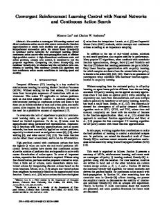
Fig. 1: A state machine of pouring behavior proposed in [Yamaguchi et al., 2015]. This is a symbolic representation of policy, and there is a corresponding hierarchical dynamic system. hierarchical dynamic system is illustrated in Fig. 1 which is a state machine of pouring behavior [Yamaguchi et al., 2015]. In the next section, we discuss about our strategy. In the succeeding sections, we summarize our recent work [Yamaguchi and Atkeson, 2016b; Yamaguchi and Atkeson, 2015].

2

A Practical Reinforcement Learning Approach in Robotic Domains

In order to introduce our strategy, first we emphasize the importance of the model-based reinforcement learning (RL) approach and symbolic representations.

2.1 Model-based RL Although the current popular approach of RL in robot learning is a model-free approach (cf. [Kober et al., 2013]), there are many reasons to use a model-based RL; dynamical models are learned from samples, and actions are planned with dynamic programming. Generalization ability and reusability There is some model-free RL work trying to increase generalization (e.g. [Kober et al., 2012; Levine et al., 2015b]). Model-based approaches can improve generalization by choosing adequate feature variables that capture the task variations. Additionally model-based approaches can reuse learned models more aggressively. Let us assume a case where the dynamics of a robot change (e.g. we switch a robot) but we still conduct the same manipulation task. The dynamics of the manipulated object do not change, thus we can expect to reuse some dynamical models without additional learning. For example in a

pouring task (cf. [Yamaguchi et al., 2015]), the dynamics of poured material flow produced by tipping a container would be common between different robots, except for a small effect caused by the robots (e.g. a subtle vibration). Another case of aggressive reuse is sharing models in different strategies. For example in pouring, there are different strategies to control flow, such as tipping and shaking a container. Sharing knowledge among strategies is possible at a detailed level with the model-based approach. For example, after material comes out from the source container and flow happens, the dynamical model between the flow state (flow position, flow variance) and the amount poured into the receiver or spilled onto a table can be shared between strategies. Such sharing or reusing would not be easy in the model-free approach. Robust to reward changes During learning a task, there are some factors causing changes of rewards, such as target changes (e.g. target positions in reaching an robot arm; i.e. an inverse kinematics problem), and reward shaping. In these situations, model-based methods would be more useful than model-free methods. Let us consider an inverse kinematics problem. We want to know joint angles q of a robot for a given target position x∗ in Cartesian space. Learning an inverse model x∗ → q becomes complicated especially when: (1) number of joints are redundant, i.e. dim(q) > dim(x∗ ), and (2) the opposite of (1), i.e. dim(q) < dim(x∗ ). In (1), there are many (usually infinite) solutions of q for a single x∗ (ill-posed problem). Handling this issue is not trivial with the model-free approach that tries to learn directly the inverse kinematics. An example of (2) is the inverse kinematics of android face (soft skin); q is displacements of the actuators inside the robotic face, and x∗ is positions of feature points (e.g. 17 points). Magtanong et al. proposed learning forward kinematics with neural networks, and solving the inverse problem with an optimization method [Magtanong et al., 2012]. This is an example of a model-based approach. They tried to learn inverse kinematics with neural networks, but the estimation becomes very inaccurate especially when some elements in a target x∗ are out of reachable range. Their model-based approach generates minimum-error solutions in such situations. Sometimes we make a goal easier to learn by manipulating the reward function. Such a way is called reward shaping (e.g. [Ng et al., 1999; Tenorio-Gonzalez et al., 2010]). This idea is also useful when a task involves multiple objectives or constraints; e.g. in a pouring task [Yamaguchi et al., 2015], the objective is pouring into a receiving container while avoiding spilling. Since reward changes do not affect the dynamical models, we can generate new optimal actions if the models are learned adequately.

models are inaccurate (this is usual when learning models), integrating the forward models represented by differential equations causes a rapid increase of future state estimation errors (cf. [Atkeson and Schaal, 1997]). We model the mapping from input to output variables of each sub-dynamical system, so that we can reduce the rapid error increase by integrals. After the task-level robot learning researches [Aboaf et al., 1988; Aboaf et al., 1989], we can consider our representation as a (sub)task-level dynamic system. We still need to estimate future states through decomposed dynamics, which will cause an error accumulation, but its speed is usually much reduced.

Symbolic Policy Representation Symbolic representation of policies is also useful. Especially in a complicated task like pouring [Yamaguchi et al., 2015], symbolic policies are essential. There are two major reasons: (A) Humans can more easily transfer their knowledge of symbolic policies to robots. (B) Symbolic policies are sharable in different domains. We implemented the pouring behavior for a PR2 robot and we could easily apply it to a Baxter robot; modifying symbolic policies were not necessary although some low-level implementations were different such as inverse kinematics and joint control [Yamaguchi and Atkeson, 2016a]. (C) A symbolic policy introduces a structure into the task. Such a decomposition increases the reusability of sub-skills. For example in [Yamaguchi et al., 2015], most sub-skills are shared between pouring and spreading. Pouring pours material from a source container to a receiver, while spreading spreads material from a source container to cover the surface of a receiver (e.g. spread butter on bread). Pouring and spreading are sharing many sub-skills; the major difference is moving the mouth of the source container to cover the surface in spreading. The symbolic policy representation enabled us to reuse many subskills between pouring and spreading.

2.3 Model-based RL with Neural Networks on Hierarchical Dynamic System

2.2 Symbolic Representations

Our strategy for RL in robotic domains is summarized as follows: (A) The robot represents high-level policies with symbolic policies, and learns them from humans. (B) The robot decomposes the task dynamics into symbols along the symbolic policies. (C) The robot learns each sub-dynamical system with numerical methods if the dynamical system is not modeled. Basically we model the mapping from input to output variables (subtask-level dynamic system). If an analytical model is available, the robot uses it. (D) The robot plans actions by solving dynamic programming over the models.

Hierarchical Dynamic Systems The aggressive model reuse as mentioned above works well when the entire dynamical system is decomposed into sub-dynamical systems. We refer to such a representation as hierarchical dynamic system. The hierarchical dynamic system is also powerful to deal with simulation biases [Kober et al., 2013]. When forward

For (D), we use a stochastic version of differential dynamic programming (DDP) to plan actions [Yamaguchi and Atkeson, 2015]. For (C), we extended neural networks to be usable with stochastic DDP [Yamaguchi and Atkeson, 2016b]. Stochastic modeling of dynamics is also helpful to deal with simulation biases.

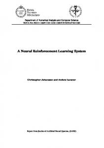
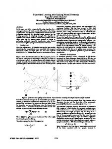
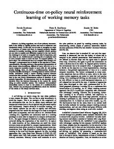
Fig. 3: A system with N decomposed processes. The dotted box denotes the whole process.

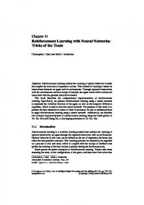
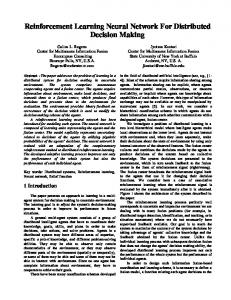
Fig. 2: Neural network architecture [Yamaguchi and Atkeson, 2016b]. It has two networks with the same input vector. The top part estimates an output vector, and the bottom part models prediction error and output noise. Both use ReLU as activation functions.

3

Neural Networks for Regression with Probability Distributions

We extended neural networks to be capable of: (1) modeling prediction error and output noise, (2) computing an output probability distribution for a given input distribution, and (3) computing gradients of output expectation with respect to an input. Since neural networks have nonlinear activation functions (in our case, rectified linear units; ReLU), these extensions were not trivial. [Yamaguchi and Atkeson, 2016b] gives an analytic solution for them with some simplifications. We consider a neural network with rectified linear units (ReLU; frelu (x) = max(0, x) for x ∈ R) as activation functions. Based on our preliminary experiments with neural networks for regression problems, using ReLU as an activation function was the most stable and obtained the best results. Fig. 2 shows our neural network architecture. For an input vector x, the neural network models an output vector y with y = F(x), defined as: h1 = f relu (W1 x + b1 ), h2 = f relu (W2 h1 + b2 ), ... hn = f relu (Wn hn−1 + bn ), y = Wn+1 hn + bn+1 ,

(1) (2) (3) (4)

where hi is a vector of hidden units at the i-th layer, Wi and bi are parameters of a linear model, and f relu is an elementwise ReLU function. Even when an input x is deterministic, the output y might have error due to: (A) prediction error, i.e. the error between F(x) and the true function, caused by an insufficient number of training samples, insufficient training iterations, or insufficient modeling ability (e.g. small number of hidden units), and (B) noise added to the output. We do not distinguish (A) and (B). Instead, we consider additive noise y = F(x) + ξ(x) where ξ(x) is a zero-mean normal distribution N (0, Q(x)). Note that since the prediction error changes with x and the output noise might change with x, Q is a function of x. In order to model Q(x), we use another

neural network ∆y = ∆F(x) whose architecture is similar to F(x), and approximate Q(x) = diag(∆F(x))2 . ∆y is an element-wise absolute error between the training data y and the prediction F(x). When x is a normal distribution N (µ, Σ), our purpose is to approximate E[y] and cov[y]. The difficulty is the use of the nonlinear ReLU operators f relu (p). We use the approximation that when p is a normal distribution, f relu (p) is also a normal distribution. We also assume that this computation is done in an element-wise manner, that is, we ignore nondiagonal elements of cov[p] and cov[f relu (p)]. Although the covariance Q(x) depends on x, we consider its MAP estimate: Q(µ).

4

Stochastic Differential Dynamic Programming

We use stochastic differential dynamic programming (DDP) proposed in [Yamaguchi and Atkeson, 2015]. Stochastic means we consider probability distributions of states and expectations of rewards. This design of evaluation functions is similar to recent DDP methods (e.g. [Pan and Theodorou, 2014]). On the other hand, we use a simple gradient descent method to optimize actions, while traditional DDP [Mayne, 1966] and recent methods (e.g. [Tassa and Todorov, 2011; Levine and Koltun, 2013; Pan and Theodorou, 2014]) use a second-order algorithm like Newton’s method. In terms of convergence speed, our DDP is inferior to second-order DDP algorithms. The quality of the solution would be the same as far as we use the same evaluation function. Our algorithm is easier to implement. Since we use learned dynamics models, there should be more local optima than when using analytically simplified models. In order to avoid poor local maxima, our DDP uses some practical methods such as multiple starting points. Fig. 3 shows a system with N decomposed processes. The input of the n-th process is a state xn and an action an , and its output is the next state xn+1 . Note that some actions may be omitted. A reward is given to the outcome state. Let Fn denote the process model: xn+1 = Fn (xn , an ), and Rn denote the reward model: rn = Rn (xn ). We assume that every state is observable. Each dynamics model Fn is learned from samples with the neural networks where the prediction error is also modeled. At each step n, a state xn is observed, and then actions {an , . . . , aN −1 } are planned with DDP so that an evaluation function Jn (xn , {an , . . . , aN −1 }) is maximized. Jn is an ex-

pected sum of future rewards, defined as follows: ∑N Jn (xn , {an , . . . , aN −1 }) = E[ n′ =n+1 Rn′ (xn′ )] ∑N = n′ =n+1 E[Rn′ (xn′ )]. (5) In the DDP algorithm, first we generate an initial set of actions. Using this initial guess, we can predict the probability distributions of future states with neural networks. The expected rewards are computed accordingly. Then we update the set of actions iteratively with a gradient descent method. In these calculations, we use our extensions of neural networks to compute the expectations, covariances, and the gradients.

5

Experiments

This section summarizes the verification of our method described in [Yamaguchi and Atkeson, 2016b]. First we conduct simulation experiments. The problem setup is the same as in [Yamaguchi and Atkeson, 2015]. In Open Dynamics Engine1 , we simulate source and receiving containers, poured material, and a robot gripper grasping the source container. The materials are modeled with many spheres, simulating the complicated behavior of material such as tomato sauce during shaking. We use the same state machines for pouring as those in [Yamaguchi and Atkeson, 2015], which are a simplified version of [Yamaguchi et al., 2015]. Those state machines have some parameters: a grasping height and pouring position. Those parameters are planned with DDP. There are four separate processes: (1) grasping, (2) moving source container to pouring location (close to the receiving container), (3) flow control, and (4) flow to poured amounts. The dimension of each state is: (2, 3, 5, 4, 2). There are 1 grasping parameter and 2 pouring location parameters. We investigated on-line learning, and compared the neural network models with locally weighted regression. After each state observation, we train the neural networks, and plan actions with the models. In the early stage of learning, we gather three samples with random actions, and after that we use DDP. Each neural network has three hidden layers; each hidden layer has 200 units. The learning performance with neural networks outperformed that of locally weighted regression. The amount of spilled materials was reduced. We also tested alternative state vectors that have redundant and/or non-informative elements. We expected automatic feature extraction with (deep) neural networks. For example we replaced a position of container by four corner points on its mouth (x, y, z respectively). Consequently the dimensions of the state vectors are changed to (12, 13, 16, 4, 2). Although the state dimensionality changed from 16 to 47, the learning performance did not change. The early results of the robot experiments using a PR2 were also positive. A video describing simulation experiments and the robot experiments is available: https://youtu.be/aM3hE1J5W98 1

http://www.ode.org/

References [Aboaf et al., 1988] E. W. Aboaf, C. G. Atkeson, and D. J. Reinkensmeyer. Task-level robot learning. In IEEE International Conference on Robotics and Automation, pages 1309–1310, 1988. [Aboaf et al., 1989] E. W. Aboaf, S. M. Drucker, and C. G. Atkeson. Task-level robot learning: juggling a tennis ball more accurately. In the IEEE International Conference on Robotics and Automation, pages 1290–1295, 1989. [Asada et al., 1996] Minoru Asada, Shoichi Noda, Sukoya Tawaratsumida, and Koh Hosoda. Purposive behavior acquisition for a real robot by vision-based reinforcement learning. Machine Learning, 23(2-3):279–303, 1996. [Atkeson and Schaal, 1997] Christopher G. Atkeson and Stefan Schaal. Robot learning from demonstration. In the International Conference on Machine Learning, 1997. [Girshick et al., 2014] Ross Girshick, Jeff Donahue, Trevor Darrell, and Jitendra Malik. Rich feature hierarchies for accurate object detection and semantic segmentation. In Proceedings of the IEEE Conference on Computer Vision and Pattern Recognition (CVPR), 2014. [Kober et al., 2012] Jens Kober, Andreas Wilhelm, Erhan Oztop, and Jan Peters. Reinforcement learning to adjust parametrized motor primitives to new situations. Autonomous Robots, 33:361–379, 2012. [Kober et al., 2013] J. Kober, J. Andrew Bagnell, and J. Peters. Reinforcement learning in robotics: A survey. International Journal of Robotics Research, 32(11):1238– 1274, 2013. [Krizhevsky et al., 2012] Alex Krizhevsky, Ilya Sutskever, and Geoffrey E. Hinton. ImageNet classification with deep convolutional neural networks. In Advances in Neural Information Processing Systems 25, pages 1097–1105. Curran Associates, Inc., 2012. [Levine and Koltun, 2013] Sergey Levine and Vladlen Koltun. Variational policy search via trajectory optimization. In Advances in Neural Information Processing Systems 26, pages 207–215. Curran Associates, Inc., 2013. [Levine et al., 2015a] S. Levine, C. Finn, T. Darrell, and P. Abbeel. End-to-end training of deep visuomotor policies. ArXiv e-prints, (arXiv:1504.00702), April 2015. [Levine et al., 2015b] Sergey Levine, Nolan Wagener, and Pieter Abbeel. Learning contact-rich manipulation skills with guided policy search. In the IEEE International Conference on Robotics and Automation (ICRA’15), 2015. [Magtanong et al., 2012] Emarc Magtanong, Akihiko Yamaguchi, Kentaro Takemura, Jun Takamatsu, and Tsukasa Ogasawara. Inverse kinematics solver for android faces with elastic skin. In Latest Advances in Robot Kinematics, pages 181–188, Innsbruck, Austria, 2012. [Mayne, 1966] David Mayne. A second-order gradient method for determining optimal trajectories of non-linear discrete-time systems. International Journal of Control, 3(1):85–95, 1966.

[Mnih et al., 2015] Volodymyr Mnih, Koray Kavukcuoglu, David Silver, et al. Human-level control through deep reinforcement learning. Nature, 518(7540):529–533, 2015. [Ng et al., 1999] Andrew Y. Ng, Daishi Harada, and Stuart Russell. Policy invariance under reward transformations: Theory and application to reward shaping. In the Sixteenth International Conference on Machine Learning, pages 278–287, 1999. [Pan and Theodorou, 2014] Yunpeng Pan and Evangelos Theodorou. Probabilistic differential dynamic programming. In Advances in Neural Information Processing Systems 27, pages 1907–1915. Curran Associates, Inc., 2014. [Pinto and Gupta, 2016] Lerrel Joseph Pinto and Abhinav Gupta. Supersizing self-supervision: Learning to grasp from 50k tries and 700 robot hours. In the IEEE International Conference on Robotics and Automation (ICRA’16), 2016. [Silver et al., 2016] David Silver, Aja Huang, Chris J. Maddison, et al. Mastering the game of go with deep neural networks and tree search. Nature, 529(7587):484–489, 2016. [Tassa and Todorov, 2011] Y. Tassa and E. Todorov. Highorder local dynamic programming. In Adaptive Dynamic Programming And Reinforcement Learning (ADPRL), 2011 IEEE Symposium on, pages 70–75, 2011. [Tenorio-Gonzalez et al., 2010] Ana Tenorio-Gonzalez, Eduardo Morales, and Luis Villase˜nor Pineda. Dynamic reward shaping: Training a robot by voice. In Advances in Artificial Intelligence – IBERAMIA 2010, volume 6433 of Lecture Notes in Computer Science, pages 483–492. 2010. [Toshev and Szegedy, 2014] A. Toshev and C. Szegedy. DeepPose: Human pose estimation via deep neural networks. In Proceedings of the IEEE Conference on Computer Vision and Pattern Recognition (CVPR), pages 1653–1660, 2014. [Yamaguchi and Atkeson, 2015] Akihiko Yamaguchi and Christopher G. Atkeson. Differential dynamic programming with temporally decomposed dynamics. In the 15th IEEE-RAS International Conference on Humanoid Robots (Humanoids’15), 2015. [Yamaguchi and Atkeson, 2016a] Akihiko Yamaguchi and Christopher G. Atkeson. First pouring with Baxter. https://youtu.be/NIn-mCZ-h_g, 2016. [Online; accessed April-15-2016]. [Yamaguchi and Atkeson, 2016b] Akihiko Yamaguchi and Christopher G. Atkeson. Neural networks and differential dynamic programming for reinforcement learning problems. In the IEEE International Conference on Robotics and Automation (ICRA’16), 2016. [Yamaguchi et al., 2015] Akihiko Yamaguchi, Christopher G. Atkeson, and Tsukasa Ogasawara. Pouring skills with planning and learning modeled from human demonstrations. International Journal of Humanoid Robotics, 12(3):1550030, 2015.