Neural Modeling and Predictive Control of a Small ...

AIAA 2012-4242

10th International Energy Conversion Engineering Conference 30 July - 01 August 2012, Atlanta, Georgia

Neural Modeling and Predictive Control of a Small Turbojet Engine (SR-30)

Downloaded by KUNGLIGA TEKNISKA HOGSKOLEN KTH on September 24, 2015 | http://arc.aiaa.org | DOI: 10.2514/6.2012-4242

Amgad M. B. Aly1, Ibrahem Atia2 Military Technical College, Cairo, Egypt

Small turbojet engines are one of the recent propulsion topics as they have many applications in aeronautics in both civil and military fields. A small turbojet engine (SR30) is tested on a Minilab test-rig. Linear ARX structure and nonlinear neural representations are used for modeling the dynamics of this small turbojet engine. This modeling is based on real engine data obtained from testing of the SR-30 engine. In order to build a feed forward neural model, one could identify the nature and characteristics of its dynamics and the order of the system to be modeled by using conventional linear system identification. This step is used to obtain a linear ARX model. Using the Input / Output relationship of this model, a neural model is trained for the SR-30 turbojet engine that represents the nonlinearity of the engine throughout its full operating range. Validation of this neural model is performed using another set of the experimental data. Neural model could capture system nonlinearity and represent the real engine dynamics. Model based Predictive Control (MPC), or simply Predictive Control, is a family of control schemes that uses a model from the plant as a predictor of the future plant outputs and hence optimize the future control inputs for the minimum future errors and minimum control energy. Among this family Generalized Predictive Control (GPC) is one of the most famous. The neural model is used in a model-based predictive control scheme. The results of this controller are compared with a classical PID controller tuned offline with a genetic optimization technique. Classical PID controller cannot cope with model variations in the whole operating range of the engine and therefore a predictive control scheme is then proposed as a solution to this problem. A neural model is used as a predictor for the calculation of GPC parameters. The nonlinear system free response is obtained by recursive future predictions while the dynamic response matrix is obtained by instantaneous linearization of the input / output relation. The results illustrate the improvements in control performance that could be achieved with a neural predicative scheme compared to that of a classical PID controller.

Nomenclature A/D ARX ARX B f G Gf Gf GSP I/O Kd Ki, Kp, logsig n Nu N1 N2 1 2

= = = = = = = = = = = = = = = = = =

Analog to digital AutoRegressive with eXternal input AutoRegressive with eXternal input bias of a neuron unit Vector of predicted free response system impulse response matrix Fuel flow rate (kg/s) Fuel flow rate (kg/s) Gas turbine simulation program Input and output derivative gain integral gain proportional gain, The sigmoid function Engine revolution speed,(rpm) Control horizon lower value of predicting horizon Higher value of predicting horizon

Lecturer, Military Technical College, Cairo, Egypt, Ph.D., [email protected] Assistant, Military Technical College, Cairo, Egypt, M.Sc., [email protected] 1 American Institute of Aeronautics and Astronautics

Copyright © 2012 by Dr. Amgad M. B. Aly. Published by the American Institute of Aeronautics and Astronautics, Inc., with permission.


NN P p PID PR R T tansig TIT tr ts W λ ˆ y u w

= Neural networks = Pressure = External input = Proportional, integral and derivative controller = Pressure ratio = Number of inputs = Sampling time = A hyperbolic tangent function = Turbine inlet temperature = Rise time = Settling time = Weight of neural networks connection = Weighting factor for control increments = Vector of predicted outputs for prediction horizon = Vector of future control increments for the control horizon = Vector of future references

I. Introduction Model Based Predictive Control (MBPC), or simply Predictive Control, is a family of algorithms with common strategy. MBPC appear in the decade of 1970s and had got a good reputation in the chemical industries and process control [1]. The main strategy of the MBPC is as follows (Figure 1). A model of the controlled system is used to predict its behaviour in the future. A known required reference trajectory is then given for certain prediction horizon. Then an optimisation algorithm is used to find the optimum control sequence for certain number of steps in the future that minimise a certain cost function which includes future predicted errors and control increments. A receding horizon technique is then applied where only the first control signal of the optimum future control sequence is applied to the controlled system.

Figure 1. Prediction strategy Generalized Predictive Control (GPC) was developed by Clarke et al. in 1987 [2]. The GPC uses ideas from Generalized Minimum Variance (GMV) [3] and is perhaps one of the most popular methods at the moment. Since the last three decades predictive control has shown to be successful in control industry. Generalized Predictive Control (GPC) was one of the most famous linear predictive algorithms. The control law of GPC contains two parameters that describe the system dynamics: system free response (f) and system impulse response matrix (G). Often these parameters are calculated from the discrete linear model. For nonlinear systems, either a nonlinear system model is instantaneously linearized or a nonlinear optimization is used. The validity of the linear model is the shortcoming of the first one and the possibility of non-uniqueness of local minimum is that for the second. The neural network (NN) model is used as a predictor to calculate these parameters for GPC. The nonlinear system free response is obtained instantaneously while dynamic response is linearized every batch of time. The method is tested on a benchmark nonlinear model. Results are compared with that of others neural predictive techniques found in previous literature. The simulation results show that this method has some good advantages over others neural predictive control techniques. In one hand, the system dynamics parameters are calculated more accurately directly from the nonlinear neural model. And in the other hand, the used linear GPC has a cost function with only one global minimum. The method [4], as a trade-off between nonlinear neural 2 American Institute of Aeronautics and Astronautics

predictive control (NPC) and instantaneous linearization approximate neural linear predictive control (APC), is promising for control of nonlinear systems. Cybenco [5] proved that a neural network with one hidden layer of sigmoid or hyperbolic tangent units and an output layer of linear units is capable of approximating any continuous function. The network is described by the magnitude of the weights and biases and should be determined by training the network on the estimation data. The estimation of the weights is usually a conventional estimation problem and several algorithms are available for this purpose.


A. Watanabe et al [6] worked on PID and fuzzy logic algorithm in order to control SR-30 turbojet engine. They obtained transfer function of the SR-30 by using frequency response method. They tested and simulated both closed loop controller PID and fuzzy logic controller. They developed their model with MATLAB environment and tested it by NI LabVIEW. R. Andoga et al [7] discussed digital electronic control of a small turbojet engine. They stated that the main purpose of control of gas turbine was increasing its safety and efficiency. Their engine was controlled by PIC 16F84A microcontroller, which manipulating the fuel flow valve. M. Lichtsinder et al [8] worked on development of a simple real-time transient performance model for AMT jet engine. The fast model is obtained using the Novel Generalized Describing Function, proposed for investigation of nonlinear control systems. The paper presents the Novel Generalized Describing Function definition and then discusses the application of this technique for the development a fast turbine engine simulation suitable for control and real-time applications. In this work, a small turbojet engine SR-30 is tested on a minilab test-rig. Then linear ARX (AutoRegressive with eXogenous input) structure and nonlinear neural network representations are used for modeling the dynamics of this small turbojet engine. This modeling is based on real engine data obtained from testing of the SR-30 engine. A feed forward neural network is then used to model the fuel flow to shaft speed relationship of a SR-30 turbojet engine. The performance of the estimated model is validated against a range of small and large signal engine tests. In order to build a feed forward NN model, one could identify the nature and characteristics of its dynamics and the order of the system to be modeled by using conventional linear system identification. This step is used to obtain a linear ARX model. Using the input/output relationship of this model, a neural model is trained for the SR-30 turbojet engine that represents the nonlinearity of the engine throughout its full operating range. Validation of this neural model is performed using another set of the experimental data This model is used in a model-based predictive control scheme. This model is linearized at different engine design points, this linearized models is used in design of a classical PID controller .the PID controller is tuned offline with a genetic optimization technique. Both controllers are tested on the SR-30 turbojet engine model and comparison is made between the results from these controllers with the same input.

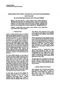
II. Testing of the SR-30 turbojet engine The NN approach was used to predict the operation of the gas turbine plant SR-30 turbojet engine. The SR30 (Figure 2) turbojet has been incorporated into many laboratories worldwide. The SR-30 engine is a turbojet engine with a single-stage radial-flow compressor with a maximum pressure ratio of, PR=3.4, a reverse-flow annular combustion chamber and a single-stage axial-flow turbine, and it operates obeying the Brayton thermodynamic cycle in the same fashion as large turbojet engines. The engine, as produced by Turbine Technologies, includes five pressure transducers, five thermocouples, a load-cell for thrust measurements, a custom motor winding for reading the engine RPM, and a fuel-flow-rate measurement system to monitor/measure the operating parameters of the engine. The engine generates 178 N of thrust at 87,000 rpm while ingesting m = 0.5 kg/s of air. The engine has a length of 27 cm, and the exit exhaust diameter of D exit= 5.715 cm.

3 American Institute of Aeronautics and Astronautics


Figure 2. SR-30 Test Rig Thirteen engine parameters are measured with the stock MiniLab configuration. The basic sensor package includes pressure, temperature, RPM and flow sensors (calibrated) measuring parameters common to Brayton Cycle type analysis. The sensors are routed to a central access panel and interfaced with data acquisition hardware and software from National Instruments. The sensor locations are shown in Figure 3. The integrated sensor system (Mini-Lab) includes the following probes: 1. Compressor inlet static pressure (P1=P 01). 2. Compressor stage exit stagnation pressure (P02). 3. Combustion chamber pressure (P3). 4. Turbine exit stagnation pressure (P04). 5. Thrust nozzle exit stagnation pressure (P05). 6. Compressor inlet static temperature (T1=T 01). 7. Compressor stage exit stagnation temperature (T02) 8. Turbine stage inlet stagnation temperature (T03) 9. Turbine stage exit stagnation temperature (T04) 10. Thrust nozzle exit stagnation temperature (T05). 11. RPM (n) engine rotational speed derived from measuring the output voltage of a generator mounted on the compressor. Additionally, the system includes a fuel flow (Gf) sensor and a digital thrust readout measuring real time thrust force based upon a strain gage thrust yoke system.

Figure 3. Sensor locations [9] The current system at the Egyptian Air forces Research Center includes a National Instruments NI PCI6031E A/D board, which has a 16-bit resolution, 100 k Samples/s sampling rate, 64 analog input, 2 analog 4 American Institute of Aeronautics and Astronautics

output, and 8 digital I/O ports. Signal connections to the A/D board are made using two enclosures, which are attached to the A/D board using cables. While one of these units (NI-SC-2345) houses the thermocouple input modules (NI-SCC-TC02), the millivolt range input modules (NISCC- AI06), a connector block for digital output signals, and the analog output modules, the other unit (NI-CA-1000) houses a connector block (NI-CB- 68LPR) to connect other analog inputs. Each input module includes self-contained signal-conditioning units such as low pass filters and instrumentation amplifiers.


While the thermocouple input modules are used to read the temperatures, the mill volt input range modules are used to read the load-cell output voltage and one of the pressure signals. Digital I/O lines are used to generate signals to turn on and off the relays. Relays (BASCO Company, ELK 924) are used to replace manual switches, which are used to start and to stop the ignition, the fuel flow and to turn on and off the valve for high-pressure air. More data about the engine can be found in [9].

A. Experiment procedure: The objective of this experiment is to measure (P01, T01, n, Gf, etc…) at different engine speeds (at steady state). Follow the “Pre-Start Checklist” and “Starting Procedure” to start the engine [10]. The turbine is inspected to insure proper rotation of the blades and to remove any debris that may get sucked into the SR-30 engine. The fluid levels are checked to insure adequate lubrication and fuel. The lab equipment iss set up by connecting an air compressor and a computer to the Mini-Lab. The air compressor is used to initiate rotation of the impeller in order to get the engine up to operating RPM range. The Virtual Bench program is used for data acquisition during a steady RPM of the engine. Steady state data are collected at different engine speeds ranging from 41,000 to 80,000 rpm. These data are used to build the engine model by using the neural networks. The following table summarizes the experimental data on the SR-30 turbojet engine Table. 1. Experiments summary

No

Date

Time

Sampling time

1. 2. 3. 4.

28/10/2009 26/10/2009 24/10/2009 24/10/2009

11:01:28 am 04:02:04 pm 02:43:46 pm 02:40:03 pm

5.

27/12/2010

03:45:08 pm

Duration

Fuel type

436 ms 436 ms 247 ms 247 ms

12 min 2.7 min 3.5 min 3.7 min

Jet A-1 Jet A-1 Diesel fuel Diesel fuel

436 ms

10.48 min

Jet A-1

Reached max TIT 0 C 780.7 750.51 640 705 715

max rpm 80,000 76,483 59,700 70,000 71,332

The following figure represents the response of engine rotational speed to random inputs in the fuel mass flow rate with jet A-1 (experiment 1).


-3

4.5

4

Experiment (1)

x 10

x 10 8 fuel flow (Gf) engine speed (n)

4

7.5

3.5

7

6.5

2.5

6


2

5.5

1.5

5

1

0.5

n (rpm)

Gf (kg/s)

3

4.5

0

100

200

300

400

500

600

4 700

Time (s)

Figure 4. The response of engine rotational speed to random inputs in the fuel mass flow rate with jet A-1

III. System identification The first and most important step in model building is to identify the nature and characteristics of its dynamics and the order of the system to be modeled. This process is called System Identification. System Identification Toolbox software lets us to estimate linear and nonlinear mathematical models of dynamic systems from measured data. We might use the resulting model to simulate the output of a system for a given input and analyze the system response, predict future system outputs based on previous inputs and outputs, or for control design. To identify a system, we must follow the following steps: 1. Data Collection 2. Model Generation 3. Minimization of errors Model generation is a multi-step process, as shown in Figure 5. It is an iterative technique, and these steps are repeated until we get the final model, a sufficiently accurate representation of the physical system.



Figure 5. Flowchart of system identification The System Identification Toolbox in Matlab software package [11] supports all pre-mentioned stapes except data collection. This toolbox provides some support for experimental design by enabling us to generate input signals with different properties. This toolbox allows the estimation of different model structures quickly; we should try as many different structures as possible to see which one produces the best results. We can also model data to validate and refine our experimental design. The identification problem in the time-domain for either linear or nonlinear modeling is to deduce relationships between past input-output data and future outputs (Identification function fid). If a finite number of past inputs u(t) and outputs y(t) are collected into the vector (t) as follows

(t )

y(y

1).........y(t

ny )u(t

1)....u(t

nu )

T

(1)

Then the problem is to understand the relationship fid between the next output y(t) and ϕ (t). To obtain this understanding a set of observed data is required which consists of the input u(t) and output y(t), from which the vector ϕ(t) can be built. The function (fid) can be linear or nonlinear function. In the case for which (f id) is a linear function several model structures are well documented such as ARX (AutoRegressive with eXogenous inputs) model. This model is parametric and has the following structure

y(t )

a1y(t

1)

...an y(t a

na )

b1u(t

nk )

...bn u(t b

nb

1)

e(t )

Where y (t) represents the output at time t, u (t) represents the input at time t, na is the number of poles, nb is the number of b parameters (equal to the number of zeros plus 1), n k is the number of samples before the input affects output of the system (called the delay or dead time of the model), and e(t) is the white-noise disturbance. The System Identification Toolbox product estimates the parameters a1 .....an and b1 .....bn using the input and output data from the estimation data set. In arxqs, na=nb=4, and nk is estimated from the step response. In our work, we use this tool to identify the system order which give the best performance. The best system is the ARX model with order [4 4 0] , na =4 and nb=4, is represented

A(q 1 )y(t )

B(q 1 )u(t )

A(q 1 )

1 1.2q

B(q 1 )

1746q

1

1

e(t )

0.1724q

946.8q

2

2

0.307q

1360q

3

3

0.3371q

1265q

4

4


(2)

So the system input will be [ y(t),y(t-1),y(t-2),y(t-3),u(t),u(t-1), u(t-2) and u(t-3)] to predict the future engine speed. The output from the ARX engine model was illustrated in the following Figure 6 which shows the comparison between the ARX model with the measured data from experiment (1). The average value of the mean square error between the model output and the experimental data is equal to 2.99 % and computation time is 0.5205 s, while the validation data running time is 664.9 s. The one second simulation time is computed in 7.8282e-004s. Linear ARX polynomial model can represent the engine with a fair accuracy. 4

8.5

ARX model response

x 10

ARX model output meassured data

7.5

7

6.5

n (rpm)


8

6

5.5

5

4.5

4

0

100

200

300

400

500

600

700

time (s)

Figure 6. Comparison between ARX model output and measured data

1. 2. 3. 4.

IV. Design of the Neural Network Topology Design of the appropriate neural network topology involves several important steps: Choosing the appropriate neurons’ transfer functions, Basic decision about the amount of neurons to be used in each layer, Selecting the amount of hidden layers.

In this paper a feed forward neural network was built to model the SR-30 engine. Function approximation has been traditionally one of the most researched uses of neural networks. Typically, a two or three layer networks are sufficient to approximate complex functions with a finite number of discontinuities. In order to gain an insight as to how topology affects the outputs, tangent sigmoid, logarithmic-sigmoid and pure linear neuron transfer functions were selected and tested for further investigation. A network topology study was conducted in order to find the most appropriate architecture neural network to fit SR-30 engine speed parameter. Note that there are several hundred combinations of neurons and layers but for practical purposes we tested four candidate topologies shown in Table 2. The training input data sets for this part of the experiment are 1018 data points selected from the engine testing and then tested (or generalized) with 370 data points selected from the same testing data. From the previous study we conclude the following result. The neural net work consists of two hidden layer with logsig function and the number of neurons in the first hidden layer is 8 and second hidden layer is 6.The function of the output layer is a linear function as shown in Table.2. This is structure of the neural networks gives minimum mean square error with value of (e=1.434 %).



Table. 2. Summary of Neural Network Training and Testing. no of hidden layer

2

2

2

2

no of neurons in first hidden layer

10

10

10

8

no of neurons in second hidden layer

10

5

1

6

Activation fn of the layer

Logsig

logsig

Logsig

logsig

Mean square error %

1.715

1.881

17.75

1.434

computation time (s)

0.12344

0.128

0.185

0.124

simulation time (s)

143.444

143.444

143.444

143.444

B.Training the Neural Network In order to simplify the analysis for development and training of the neural network models the MATLAB Neural Network Toolbox is employed [12]. This tool is very efficient to handle matrices and is used throughout this research project to handle data manipulation tasks and neural network computations.

C. Selection of Training Algorithms Based on the analysis performed with several transfer functions in the neural network the LevenbergMarquardt algorithm was found to be the most efficient and reliable means to be used for this study. The neural network employed in the SR-30 model is based on non-linear optimization techniques. The objective of the optimization is to train the network parameters weights (w) and biases (b) so they can be adjusted in an effort to optimize the performance of the network. Neural networks are taught to accommodate changes in the weights and biases to appropriately reconfigure the output. During each training operation the error between the output and target becomes smaller until a minimized error goal is achieved. These weighs and biases are somewhat equivalent to the regression constants found in many nonlinear multivariate estimation models and thus can be easily incorporated in any programming environment that supports array manipulation. The experimental data from experiment (1) is used for network training. The results of the neural net work training were shown in Figure 8-Figure 7. The average value of the mean square error between the model output and the experimental data was equal to 0.9025 % and the model computation time is 0.5066 s while the measured data running time is 664.9 s. The one second simulation time is computed in 7.6192e-004 s. i.e. this model could be considered as a real-time simulation model. If this model simulation time is still less than the actual time then, time delays must be added to the model to make its behavior near real.


4

8

Neural model training

x 10

Neural model output experimental output 7.5

7

6.5

5.5

5

4.5

4

3.5

0

100

200

300

400

500

600

700

time (s)

Figure 7. Comparison between neural output and measured data -3

4.5

Neural model training

x 10

4

3.5

3 Gf (kg/s)


n (rpm)

6

2.5

2

1.5

1

0.5

0

100

200

300

400

500

time (s)

Figure 8. Input measured data 10 American Institute of Aeronautics and Astronautics

600

700

D. Validation of the neural network data The validation of the neural model is performed with a different input data to check the accuracy of the model. The experimental data from experiment (2) is used for network validation. The result of the validation process is shown in Fig (9) Fig (10). The average value of the mean square error between the model output and the experimental data is equal to e=1.473 %. -3

5

Neural model validation

x 10

Gf (kg/s)

3

2

1

0

-1

0

50

100

150

time (s)

Figure 9. Measured data used for model validation 4

8

neural model validation

x 10

Neural network model output experimental output

7.5

7

6.5

6

n (rpm)


4

5.5

5

4.5

4

3.5

3

0

50

100 time (s)

Figure 10. Validation data results 11 American Institute of Aeronautics and Astronautics

150

A comparison between the neural model and ARX linear model with the same data was shown in Figure 11 and it is clear that the neural model can simulate the engine dynamics through its operating rang with good accuracy.

4

8.5

Model comparison

x 10

ARX model output Neural model output experimental output

8

7.5

6.5 n (rpm)


7

6

5.5

5

4.5

4

3.5

0

100

200

300

400

500

600

700

time (s)

Figure 11. Comparison between ARX and neural model with experimental data

V. Turbojet engine controller design For a gas-turbine engine, particularly for a jet engine, the speed (n) control is one of the most important aspects (even most important than the engine’s temperature control) and it’s currently realized by some specific hydro-mechanical or electro-mechanical controllers. The engine’s speed is the most important operating parameter, especially for the multi-spool engines, because it represents the parameter which assure the most accurate co-relation with the engine’s thrust amount, as well as with the engine’s fuel consumption; meanwhile, the speed n offers an image about the dynamic load of the engine’s mobile parts (compressor’s blades and disks, turbine’s blades and disks, shafts), as well as an indirect image about the thermal charge of the engine’s hot parts (combustor, turbine(s), exhaust nozzle). An aircraft engine operates at various flight regimes, that means at various flight speed and flight altitudes, which means that the engine’s thrust variation must follow the aircraft flight dynamic’s necessities, therefore the engine’s speed (and thrust) must be strictly controlled, because of its important operating role. The engine’s speed is one of the engine’s operating parameters, which are the easiest to measure, both for steady state regimes and for dynamical regimes. That fact represents an advantage and promotes the engine’s speed as the most important controlled engine’s parameter. In this paper an engine speed controller has been studied with fuel flow rate as a regulating parameter. The controller design is based on engine neural networks model.



E. Discrete PID based on engine NN model The discrete PID controller was used with the NN model of the SR-30 turbo jet engine. Now, the tuning of the PID is achieved by using genetic algorithm. The GA is carried out using a MATLAB built-in routine so called Simulink Response Optimization (SRO) Toolbox as shown in Figure 12. The SRO, automatically, formulates an optimization problem and calls a genetic algorithm and direct search toolbox, as an optimization routine to solve the problem.

Figure 12. Simulink Response Optimization (SRO) Toolbox A classical discrete PID control system can be described as shown in which the input-output relation of the PID controller is expressed mathematically by equation (3)[13]. N

u(t )

K p e(t )

TK i

e(t ) t 0

Kd

e(t )

e(t T

1)

(3)

where, u(t) is the control signal, e(t) is the error signal, and Kp, Ki, and Kd denotes the proportional gain, integral gain and derivative gain respectively, T is the sampling time and N is the number of samples, u (t) represents the output of the of the controller at the sampling point (t). If the sampling period is short enough, the approximate calculation by equation (3) can get an accurate result and the discrete control process is close to the continuous control process. The digital PID Controller transfer function as a function of z has the following form [13]

C (z )

Kp

KiT

z z

1

Kd z 1 T z

Where: Kp, Ki and Kd are the proportional, integral and derivative parameters of the controller and ‘T’ the sampling time. The required step response characteristics of the engine are rise time (t r) = 0.872 s, settling time (ts) = 4 s and maximum overshoot (Mp) = 2%. PID controller is tuned, based on the linearized neural model (equation(5)). The linearization is performed at different operating points; with step change from 41050 to 82000 rpm (5) A(q 1 ) y(t ) B(q 1 )u(t ) Where

A(q1 )  1  a1q1  ..............  ana q  na B(q1 )  bo  b1q1  ..............  bnb q nb


(4)

y(t) and u(t) are the current output and input signals, respectively. The coefficients of the extracted linear models can be calculated by the derivative of the future output y(k+1) against each input p=[ y(t),y(t-1),y(t2),y(t-3), u(t),u(t-1), u(t-2) ,u(t-3)] [15]. For a two hidden layer with logsig function and linear output layer, the predicted output from the neural network based on the past inputs and outputs is presented in the following equation yˆ(k  1)  w o  logsig[ w2  logsig[w1  p  b1 ]  b 2 ]  b3 (6) The derivative of the output yˆ(k  1) with respect to specific input pi is calculated as shown in the following equation.      yˆ (7) logsig[ w(2)  logsig[ w(1)  p  b1 ]  b 2 ]    w 2   logsig[ w1  p  b1 ]   w1  w (0)   pi





pi 

 





Where w  , w  , w  are the weight matrices of the neural model and b  , b  , b  are the bias vectors of the layers of the neural model. Where the sigmoid function (logsig) is presented by the following equation. 1 (8) logsig( x) 1 e( x ) 0


 pi

1

2

0

1

2

The derivative of the sigmoid function is presented by the following equation.

 e x log sig ( x)  x (1  e x )2

(9)

p is the input vector to the neural network which consists of the past input and output (equation (10)). p  u  t  u  t  1 u  t  2  u  t  3 y  t  y  t 1 y  t  2  y  t  3 

(10)

The derivative of the output yˆ(k  1) with respect to uk is equal to  b0 ,b1 ,b2 ,b3  and The derivative of the

output yˆ(k  1) with respect to y(k) is equal to 1, a1, a 2 , a 3 , a 4  . Table 3 represents the linearized neural model at different operating points along the engine operating line. Table (3) Linearized neural models The engine operating speed (rpm) 41050 46050 51060 56050 61050 66060 71060 76100 82000

The linearized neural model transfer function (

4.654e006  8.289e005 z 

1  0.6219 z



1  0.6425z 1  0.6021z



4.354e006  1.864e006 z 

1

1  0.3624 z



1

1  0.205 z





1



1

1  0.2332 z



1









2



2

2



 0.1692 z 2



2

 0.01691z

 0.03123z

2





2

 4.902e005 z



3

 0.1269 z



 0.09487 z

 2.145e006 z 

3

3

4

4

 9.956e005 z 3



3

 0.08725 z

3

2

2



 2.935e005 z

2





3

4

 0.1254 z 

3

4



 0.1166 z

 0.05855 z




3







3

4

 3.938e005 z

3 

 0.1026 z

 0.08678 z

3

 2.97e005 z

2 

 6.618e005 z 

 2.499e005 z

 0.1573z 



2

2





 0.04286z



 0.129 z

 2.036e004 z

1

1



 7.189e005 z

1

 0.07119 z

1.571e006  2.068e006 z



 1.092e006 z

3

4

3



 0.1127 z

 7.289e005 z

1

 0.04814 z

5.047e006  5.383e006 z 1  0.3787 z

2

 1.158e006 z

1

3.392e006  4.278e006 z 1  0.1673z







 0.0076z

3

2



 0.1057 z

 1.027e006 z

1

 0.01317 z

1



 0.004585 z

3.36e006  4.051e006 z 

2

 0.01549 z

3.917e006  2.889e006 z



 1.434e006 z

1

 0.05878 z

1

1  0.5084 z







 1.645e006 z

2

 0.09764 z

2

 1.845e006 z

1



4.642e006  7.661e005 z 



 0.08984 z

1



 2.016e006 z

1

 0.1028z

1

4.821e006  2.107e005 z 



n ) Gf

 0.1532 z





3

4 

 

3 4

3

4

Different controller types are used such as P, PI, and PID controller to determine the best type of controller. The optimal P,PI and PID controller parameters after optimization are shown in (Table 3) using small-amplitude step inputs, to cover the engine operating ranges in which the data used for the estimation and validation are available. Table (3) PID parameters at different step changes based on linearized neural network model Step changes (rpm)


41050-46050

46050-51060

51060-56050

56050-61050

61050-66060

66060-71060

71060-76100

76100-80000

Type of controller

kp

ki

kd

MSE (%)

P PI PID P PI PID P PI PID P PI PID P PI PID P PI PID P PI PID P PI PID

28 8.7026 9.3614 33 13.3843 7.6575 28 5.5286 5.5169 25 6.2435 3.8647 22.5 4.932 2.9938 18.5 8.3053 5.1222 12.5 5.2974 4.7983 15.5 2.8438 2.2171

0 7.6406 8.225 0 10.956 7.9768 0 8.9534 8.9447 0 12.3337 10.0165 0 13.1443 11.8407 0 18.6432 13.8288 0 18.1128 17.0898 0 14.1248 14.4599

0 0 0.7027 0 0 0.2169 0 0 0 0 0 0.1051 0 0 0.4457 0 0 1.0927 0 0 1.3843 0 0 2.4557

1.776 0.3213 0.2626 1.602 0.1674 0.2537 1.593 0.2826 0.3447 1.757 0.2546 0.3177 1.983 0.3324 0.3843 2.1 0.2927 0.1676 2.599 0.6919 0.1406 1.731 0.2607 0.1124

As can be seen from (Table 3), the PID controller gives the smallest error when used near to the ideal and maximum speed. The PI controller gives the smallest error when used in engine speed range from n = 46050 to 66060 rpm. The engine controller must be accurate when operates near to maximum speed to avoid engine damage and also near to ideal speed to avoid the engine flame out. So that, PID controller is selected to control the SR-30 engine. The resulted step response shown in Error! Reference source not found., represents the engine response with a step input from n=76100 to 80000 rpm. For P controller there is a steady-state error. The proportional gain is increased to reduce steady-state error, but the system will begin to oscillate. Thus, Kp must be selected suitable to make the system stable and have the effect of reducing the rise time and steady-state error. This steady state error is eliminated when using PI controller but the maximum over shoot percentage increases and the settling time is also increase. To reduce the maximum over shoot percentage and settling time, PID controller is used.


-3

4.7

Engine step response

x 10

P controller input PI controller input PID controller input

4.6

4.5

Gf (kg/s)

4.4

4.3

4.1

4

3.9

0

2

4

6

4

8.1

8

10 time (s)

12

14

16

18

20


x 10

P controller output PI controller output PID controller output reference output

8.05

8

7.95

7.9

n (rpm)


4.2

7.85

7.8

7.75

7.7

7.65

7.6

0

2

4

6

8

10 time (s)

12

14

16

18

20

Figure 13. Engine response with step change from n=76100 to 80000 rpm The response of the engine with different types of input is obtained in order to check the robustness of the PID controller. Figure 14 represents the comparison between the response of the engine due to step input from n=76100 to 80000 rpm with PID controller tuned with engine speed from n=76100 to 80000 rpm and PID controller tuned with engine speed from n=61050 to 66060 rpm. As can be seen from this figure, the system response with PID controller tuned in the same range of the input signal is better than the system response with PID controller tuned in different range.


-3

4.6


x 10

4.5

4.4

PID 61050 input PID 76100 input

Gf (kg/s)

4.3

4.1

4

3.9

0

2

4

6

4

8.05

8

10 time (s)

12

14

16

18

20


x 10

8

7.95 PID 61050 output PID 76100 controller output reference output

7.9

7.85

n (rpm)


4.2

7.8

7.75

7.7

7.65

7.6

0

2

4

6

8

10 time (s)

12

14

16

18

20

Figure 15. Comparison between engine responses with two different PID controllers The response of the system with PID controller tuned in the same range of input signal has less rise time, setting time and maximum over shoot percentage than the system response with PID controller tuned in different range. This is due to the fact that the PID controller is a linear controller. It is thus not capable of dealing optimally with a nonlinear constrained system across its whole operating range. Also Figure 16 represents the engine response with PID controller tuned at n=76100 rpm, the curve shows that the settling time and maximum overshoot percentage are decrease as the deviation from the tuned point (no= 76100 rpm) decrease and increase as the deviation from the tuned point increase


-3

5.5

PID controller input

x 10

5

4.5

4

Gf (kg/s)

3.5

3

2.5

1.5

1

0.5

0

10

20

30

4

8.5

40

50 time (s)

60

70

80

90

100


x 10

PID 76100 output reference output

8

7.5

7

6.5

n (rpm)


2

6

5.5

5

4.5

4

0

10

20

30

40

50 time (s)

60

70

80

90

100

Figure 17. Engine response with different steps change from n=61050 to n=81000 The system nonlinearity is well illustrated if an increasing amplitude square pulse signal is given to the system. Figure 18 shows the response of the engine in case of square pulse signal input with the PID controller that is tuned at n =61050 rpm. There is an over shoot in the engine response


-3

4.4

PID controller input

x 10

4.2

4

3.6

3.4

3.2

3

2.8

0

100

200

4

7.8

300 time (s)

400

500

600

Engine response

x 10

PID 61050 output reference output 7.6

7.4

7.2

7

n (rpm)


Gf (kg/s)

3.8

6.8

6.6

6.4

6.2

6

0

100

200

300 time (s)

400

500

600

Figure 19. The response of the engine in case of square pulse signal input with the PID controller The parameters of the PID controller must be changed. Hence, the PID controller without gain-scheduling is not an effective controller for this kind of nonlinear systems. The need is therefore apparent to design a global controller across its whole operating range, and there is a need to implement nonlinear controller designs. This study will now consider Model based Predictive Controller (MPC).

F. Model Predictive Controller In order to implement the predictive controller strategy, the basic structure shown in Figure 20 is used. A model is used to predict the future plant outputs, based on past and current values and on the proposed optimal future control actions. These actions are calculated by the optimizer taking into account the cost function (where the future tracking error is considered) as well as the constraints.



Figure 20. Basic structure of MPC Model based Predictive Control (MPC) is families of control schemes that uses a model from the plant as a predictor of the future plant outputs and hence optimize the future control inputs for the minimum future errors and minimum control energy. Among this family Generalized Predictive control (GPC) is one of the most famous. The basic idea of GPC is to calculate a sequence of future control signals in such a way that it minimizes a multistage cost function defined over a prediction horizon. The index to be optimized is the expectation of a quadratic function measuring the distance between the predicted system output and some predicted reference sequence over the horizon plus a quadratic function measuring the control effort. GPC provides an explicit solution (in the absence of constraints), it can deal with unstable and no minimum phase plants and incorporates the concept of control horizon as well as the consideration of weighting of control increments in the cost function. The general set of choices available for GPC leads to a greater variety of control objectives compared to other approaches, some of which can be considered as subsets or limiting cases of GPC. The GPC algorithm consists of applying a control sequence that minimizes a multistage cost function J: N2

J

yˆ k

j

w k

Nu

2

j

j N1

Subject to:

u k

j

j

1

2

(11)

j 1

0 for N u

1

u k

j

N 2 ,where N1 denotes the minimum prediction horizon, N2 the

maximum prediction horizon and Nu the control horizon, λ is a weight factor penalizing changes in the control input to obtain smooth control input signals and d is the system time delay. Then the predictor equation becomes in matrix form ˆ G u y

f

(12)

Where:

ˆ y

yˆ k

yˆ k

N1

gN gN

0

1

gN

1

1

N1

yˆ k

1

0

0

u

0 0

2

gN

u k f

2

0 0 gN

1

u k f k

T

1

G gN

N2

u k

1

N1

f k

N2

2

Nu 1

Nu

1

T

T

Then J could be written in matrix form as: J

ˆ y

w

T

ˆ y

w

uT u


(13)

Where:

w Minimize

J to get optimum

w k

N1

w k

T

N2

u we get: u*

GT G

I

1

GT

w

f

(14)

Taking the first element of the control sequence (as the receding horizon principle) u* k H w f

(15)

Where:


H

1 0 0

0

T

GT G

I

1

GT

For a linear time-invariant system the parameter H is unchanged over the time. But the free response f should be calculated every time step. The incremental controller ensures zero offsets even with non-zero constant disturbance. The choices of parameters ( N 1, N 2 , N u and ) determine the stability and performance of the GPC controller. Some guidelines for selecting them exist in [14-15]. Free System Response ( f )

ˆ then the output To get the free system response the prescribed NN is given a zero increment vector u ˆ will be the system free response f . predicted vector Y Impulse system response ( G ) The impulse response of the system is calculated using trained NN model with a linearization around the current operating point. To get the first column of the G matrix a small value for uˆk 1 is assumed as small value , where

1 and the corresponding output prediction is obtained. ˆ u 0 0 0

(16)

Then the first column of the G matrix will be G1

1

ˆ (Y

f)

(17)

It will be easy after that to form the special shape of G matrix then calculate H vector. G. Neural Predictive controller scheme (NNGPC) The used control scheme [4] consists of a nonlinear neural network model in the form of NN model and a linear GPC controller. The neural model is trained off-line within the complete range of system input. After performing the training, the network is then used by the GPC controller to calculate the free response of nonlinear system every time step. Every batch of time the impulse response matrix is calculated through linearization. The control law (15) is computed every time-step to get the next control increment.

Figure 21. Proposed Neural Network GPC Control Scheme 21 American Institute of Aeronautics and Astronautics

Application to the SR-30 NN model The predictive controller parameters are N 1

1 , N2

4 , Nu

1,

0.05

The system nonlinearity is well illustrated if an increasing amplitude square pulse signal is given to the system. The Simulations results and Comparison with the PID controller with the same input will be illustrated below. Figure 22 shows the engine response with a step input from n=76100 to 80000 rpm. The mean square error between the reference output and the system output is 0.001637. 4

8.05

The engine response

x 10

The Predictive controller reference data

7.95

7.9

n (rpm)

7.85

7.8

7.75

7.7

7.65

7.6

0

2

4

6

8

10 time (s)

12

8

10 time (s)

12

14

16

18

20

-3

4.6

x 10

4.5

4.4

Gf (kg/s)


8

4.3

4.2

4.1

4

3.9

0

2

4

6

14

16

18

20

Figure 22. Engine response with step change from n=76100 to 80000 rpm for predictive controller controller input

VI. Results of comparison between PID controller and predictive controller In this section, the response of the engine with different types of input is obtained in order to check the robustness of the predictive controller, and comparison between the responses of the engine with predictive and PID controller is with the same input performed. Figure 23 represents the comparison between the response of the engine due to step input from n=41050 to 80000 rpm with predictive controller, PID controller tuned with engine speed from n=76100 to 80000 rpm. The PID controller has a higher over shoot and settling time than the predictive controller.


4

10

PID and precdictive controller comprison

x 10

predictive Controller PID 76100 Controller Refernce output 9

n (rpm)

8

7

5

4

0

2

4

-3

6

6

8

10 time (sec)

12

14

16

18

20


x 10

predictive Controller input PID 76100 Controller input

5.5

5

4.5

4

Gf (kg/s)


6

3.5

3

2.5

2

1.5

1

0

2

4

6

8

10 time (sec)

12

14

16

18

20

Figure 24. Engine response with step change from 41050 to 80000 rpm Also Figure 25 represents the comparison between the response of the engine due to different steps change from n=61050 to n=81000 with predictive controller and with PID controller tuned at n=76100 rpm. The system response with predictive controller has the smallest settling time, over shoot and response oscillation.


4

8.5


x 10

predictive Controller PID 76100 Controller Refernce output

8

7.5

7

n (rpm)

6.5

6

5

4.5

4

0

10

20

-3

5.5

30

40

50 time (sec)

60

70

80

90

100


x 10

predictive Controller input PID 76100 Controller input

5

4.5

4

3.5

Gf (kg/s)


5.5

3

2.5

2

1.5

1

0.5

0

10

20

30

40

50 time (sec)

60

70

80

90

100

Figure 26. Engine response with different steps change from n=61050 to n=81000 Figure 27 shows the response of the engine in case of square pulse signal input with the PID controller that is tuned at n =61050 rpm.


4


x 10

8.2

predictive Controller PID 61050 Controller Refernce output

8 7.8 7.6

n (rpm)

7.4 7.2 7 6.8 6.6

6.2 6

0

100

-3

4.4

200

300 time (s)

400

500

600


x 10

predictive Controller input PID 76100 Controller input 4.2

4

3.8

Gf (kg/s)


6.4

3.6

3.4

3.2

3

2.8

0

100

200

300 time (sec)

400

500

600

Figure 28. The response of the engine in case of square pulse signal input Finally, it can be therefore concluded that the parameters in the PID controller parameters need to be changed with the operating range, but using predictive controller enables a global controller to be implemented and provides the optimal control performance across the operating range. Predictive controller provides the best control performance in the presence of disturbances and model uncertainties. Also, as can be seen from this comparison between the predictive controller and PID controller, the control energy in case of predictive controller is smaller than the control energy in case of PID controller. This means that the effort required to reach the steady state response [curves of Gf versus time] is smaller in case of predictive controller. This result also affects on the life time of the fuel metering valve that controlled by the controller unit. In case of predictive controller the required movements of the fuel metering valve spool is smaller than the movements in case of PID controller. Also the oscillation in the motion of the metering valve is smaller in the case of predictive controller

VII. Conclusion A representative neural network SR-30 engine model was developed using data given from the testing of the engine. The neural network is trained to estimate the engine revolution speed (n) as a function of the fuel flow rate (Gf). Results from the neural model are compared to the actual performance provided in engine testing data with mean square error of value (0.9025 %). The results are adequate for the implementation in real-time simulation where the model computation time is 0.5066 s while the measured data running time is 664.9 s. The following conclusions are derived from our analysis: 25 American Institute of Aeronautics and Astronautics


1. 2.

The model developed in this research project purely addressed the SR-30 engine The information provided from the testing of the engine is a reliable source to study the performance of the SR-30 turbojet engine. 3. The system identification results obtained in this paper indicate that linear ARX polynomial model can represent the engine with a fair accuracy 4. Along with neural network technology, a neural network model has been developed. Results obtained from the neural network engine model show that a neural network with proper training is an accurate and efficient mean to calculate the engine speed. Neural networks can approximate with good accuracy the dynamics of the engine through its operating range. 5. The comparison made with the results obtained from the linear ARX model and nonlinear neural model shows clearly the superiority of neural networks as a tool in nonlinear system modeling. 6. The neural networks model cannot be build during the early phase of the engine design because the neural model needs a measured data from the engine to be modeled.. A representative neural network SR-30 engine model was used to develop a PID controller and predictive controller. Results from the two controllers were compared and predictive controller found to be accurate for engine control during the full operating rang. The following results are derived from our analysis: 1. PID controller was built based on the neural networks model of the SR-30 engine. 2. Tuning of the PID controller was performed with offline with a genetic optimization technique. 3. PID controller cannot cope with model changes in the whole operating range of the engine. 4. A neural model was used as a predictor for the calculation of GPC parameters. The nonlinear system free response was obtained by recursive future predictions while the dynamic response matrix was obtained by instantaneous linearization of the input /output relation. 5. As a conclusion, the results illustrate clearly the improvements in system performance that could be achieved with a neural predicative controller compared to that of a classical PID controller.

VIII.

References

[1] Garcia C.E. , Prett D.M. , and M. Morari,“ Model predictive control: theory and practice- a survey ,” Automatica, 25(3): 335-348, (1989). [2] D.W. Clarke, C Mohtadi, and P.S. Tuffs. “Generalized Predictive Control. Part I. The Basic Algorithm. Automatica” 23(2):137-148, 1987. [3] D.W. Clarke and P.J. Gawthrop. “Self-tuning Control. Proceedings” IEEE, 123:633-640,1979. [4] A.M. Bayoumy, J. Bordeneuve-Guibé , “A Neural Predictive Control Scheme For Nonlinear Plants”, AIAA paper 2002-1541. [5] Cybenco, G., “Approximation by superpositions of a sigmoidal function,” Mathematics of Control, Signals, andSystems, 2, 4, pp. 303-314. 1989, [6] Watanabe, A., lmen, S. M., Leland, R., Whitaker, K. W., and Trevino, L. C., 2004, “Soft Computing Applications on SR-30 Turbojet Engine” AIAA Paper No. 2004–6444. [7] Andoga, Rudolf, Ladislav Madarasz, and Ladislav Fozo. "Digital Electronic Control of a Small Turbojet Engine - MPM 2." 12. International Conference on Intelligent Engineering Systems. Miami, Florida. 37-40, 2008. [8] Michael Lichtsinder, Yeshayahou Levy “Jet Engine Model for Control and Real-Time Simulations” Journal of Engineering for Gas Turbines and Power, 2006 by ASME, October 2006, Vol. 128 / 745. [9] Chicago, “Mini-Lab SR-30 Gas Turbine Engine Document”, Turbine Technologies, Chetek, WI, 2004. September 20-22, 2004. [10] Gas Turbine Power System Operator's Manual Turbine Technologies, LTD, 2006 [11] System Identification Toolbox User’s Guide, the Mathworks, Feb 2010. [12] Neural Network Toolbox User’s Guide, the Mathworks, Feb 2010. [13] Charles L Phillips, “Digital control system analysis and design” Prentice-Hall, Englewood Cliffs, New Jersey, 1984. [14] Clarke D.W., C. Mohtadi and P.S. Tuffs,“ Generalized Predictive Control. Part2: Extensions and interpretations,” Automatica, vol.23, Nº2, pp. 149-160, (1987) [15] Clarke D.W. and C. Mohtadi ,“Properties of generalized predictive control” Proceedings of the 10th triennial world congress of IFAC, Munich, FRG, pp. 65-76, (1987). [16] J. Mu et al. “Advanced controller design for aircraft gas turbine engines”, Control Engineering Practice 13, 1001– 1015, 2005.


Neural Modeling and Predictive Control of a Small ...

Neural Modeling and Predictive Control of a Small ...

Suggest Documents

A Neural Predictive Control Scheme for Small

Generalized Predictive Control and Neural Generalized Predictive ...

Modeling and Predictive Control of a Cash

Nonlinear Multivariable Predictive Control: Neural

Neural Network Modeling and Nonlinear Predictive ...

NEURAL PREDICTIVE CONTROL TOOLBOX FOR

Neural Generalized Predictive Control: A Newton ... - CiteSeerX

A Predictive Modeling Based on Regression and Artificial Neural ...

Modeling and Predictive Control of a Rotating Disk Bioreactor

Building modeling and identification for predictive control

Neural Network Predictive Control of a Chemical Reactor

Neural Network-Based Model Predictive Control of a Servo-Hydraulic ...

Neural Network Predictive Control of a SOFC Fuelled with Ammonia

Neural Network Predictive Control of a Chemical Reactor

Neural Network Predictive Control of a Chemical Reactor

NEURAL PREDICTIVE CONTROL TOOLBOX FOR ...

Neural Network Based Model Predictive Control

NONLINEAR PREDICTIVE CONTROL BASED ON NEURAL MULTI

Adaptive Neural Model-Based Predictive Control

Neural Network Predictive Control for Autonomous Underwater

Neural Network Based Model Predictive Control

Simulink Blockset for Neural Predictive Control - ace.ucv.ro

Modeling and Control of a Small-Scale Hybrid Aircraft

Modeling, Control, and Flight Testing of a Small ... - Semantic Scholar