Numerical simulation of particulate- flow in spiral separators - RACO

Numerical simulation of particulateflow in spiral separators (15 % solids) Mahran, G. M. A.*1, Doheim, M. A.**, AbdelGawad, A.F***,2, Abu-Ali, M. H.**, Rizk, A.M.** * King Abdulaziz University, Jeddah 21589,Saudi Arabia. Mining and Metallurgical Eng. Dept., Faculty of Engineering, Assiut University, Egypt. *** Mechanical Power Eng. Dept., Faculty of Engineering, Zagazig University, Egypt. 2 Currently: Mech. Eng. Dept., Umm Al-Qura University, Makkah, Saudi Arabia

**

AFINIDAD - Article núm.: 4133

Numerical simulation of particulate-flow in spiral separators (15 % solids) ***,2 ** Mahran,Simulación G. M. A.*1, Doheim, M. A.**, del AbdelGawad, , Abu-Ali, H.**separador , and Rizk, A.M. numérica flujo deA.F partículas enM.un espiral (15 % de sólidos) * King Abdulaziz University, Jeddah 21589,Saudi Arabia. ** Mining and Metallurgical Eng. Dept., Faculty of Engineering, Assiut University, Egypt. *** Simulació numèrica del fluix de partícules en un separador d’espiral (15% de sòlids) Mechanical Power Eng. Dept., Faculty of Engineering, Zagazig University, Egypt. 2 Currently: Mech. Eng. Dept., Umm Al-Qura University, Makkah, Saudi Arabia

AFINIDAD - Article núm.: 4133

Recibido: 6 de febrero 2014; revisado: 7 de octubre de 2014; aceptado: 5 de noviembre de 2014 Simulación numérica del flujo de partículas en un separador espiral (15 % de sólidos)

Numerical simulation of particulate-flow in spiral separators

G. sòlids) M. A.*1, Doheim, M. A.**, AbdelGawad, A.F***,2, Abu-Ali, M. H.**, Simulació numèrica del fluix de partícules en un separador d'espiralMahran, (15% de *

King Abdulaziz University, Jeddah 21589,Saudi Arabia. Mining and Metallurgical Eng. Dept., Faculty of Engineering, Assiut Univ *** Mechanical Power Eng. Dept., Faculty of Engineering, Zagazig Unive 2 Currently: Mech. Eng. Dept., Umm Al-Qura University, Makkah, Sau

**

Recibido: 6 de febrero 2014; revisado: 7 de octubre de 2014; aceptado: 5 de noviembre de 2014

Simulación numérica del flujo de partículas en un separador espira

1

*Corresponding author: [email protected]

RESUMEN AFINIDAD - Article núm.: 4133 ElRESUMEN separador espiral es un dispositivo de concentración

Numerical simulation particulate-flow in spiral separators por gravedad. of Fue inventado por Humphreys in 1941.Ha(15 %

tion and concentration of particulates on the spiral trough. The predicted results are compared the experimental Simulació numèrica del fluix dewith partícules en un separador d'espiral (1 in case LD9 coal spiral. Comparisons between numerical solids) and measured data show good agreement.

sido diseñado y desarrollado en base a la experiencia y El separador espiral **es un dispositivo de***,2 concentración por**gravedad. Fue Recibido: inventado por 6 de febrero 2014; revisado: 7 de oc ** a la gran variedad modificaciones. El H. ob-, and Rizk, Key words: Spiral separator, particulate-flow, numerical Mahran, G. M. A.*1 , Doheim, M. A.de, prototipos AbdelGawad,y A.F , Abu-Ali, M. A.M. * Humphreys in 1941.Ha sido diseñado y desarrollado en base a la experiencia y a la gran King Abdulaziz University, Jeddahes 21589,Saudi Arabia. jetivo principal del presente estudio la simulación del simulation, turbulence modeling, gravity separation, CFD. 2014; aceptado: 5 de noviembre de 20 ** variedad de prototipos y modificaciones. objetivo principal del presente Mining flujo and Metallurgical Eng. Faculty of Engineering, Assiut University, Egypt. estudio es la de partículas de Dept., concentraciones deElsólidos más rea*** Mechanical Power Eng. Dept., Faculty of Engineering, Zagazig University, Egypt. simulación del flujo de partículas de concentraciones de sólidos más reales (15% de sólidos les (15% de sólidos en peso) en un separador espiral. El 2 *Corresponding author:[email protected] Currently: Mech. Eng. Dept., Umm Al-Qura University, Makkah, Saudi en peso) unbasado separador El estudio se ha basado en el Arabia método Eulerian y el modelo estudio seenha enespiral. el método Eulerian y el modelo RESUM en en laslas características del flujo de partículas deturbulencia turbulencia RNG K-𝜺𝜺𝜺𝜺.. Los de Los resultados resultadossesecentran centran características del de partículas como la velocidad y (15 % separador d’espiral comonumérica la velocidad yflujo la distribución y en concentración deespiral partículas enUn laRESUMEN curvatura espiral. Los és un dispositiu de concentració Simulación del flujo de partículas un separador de sólidos) laresultados distribución y concentración de partículas en la curvaper inventat per Humphreys en 1941. Va pronosticados se comparan con los valores experimentales engravetat. el caso deVa unaser espiral tura espiral. Los resultados pronosticados dissenyat i desenvolupat en primer lloc sobre la base de carbón tipo LD9. Las comparaciones entre se los comparan datos numéricos yser los medidos coinciden El separador espiral es un dispositivo de concentración por gravedad. Fue in los valores experimentales en un el separador caso de una espiral de l’experiència i a través de moltes proves de prototips Simulaciócon numèrica del fluix de partícules en d'espiral (15% de sòlids) bastante. Humphreys in 1941.Ha sido diseñado y desarrollado en base a la experienc de carbón tipo LD9. Las comparaciones entre los datos i modificacions. L’objectiu principal d’aquest estudi és la variedad del de prototipos y modificaciones. El objetivo numéricos y los medidos coinciden bastante. simulació fluix de partícules de concentració de principal sòlids del presente Palabras clave: Separador de espiral, flujo de partículas, simulaciónmés numérica, modelo de simulación del de flujo de partículas sólidos más reales real (15% sòlids en pes)de enconcentraciones un separador de d’esturbulencia, separación por gravedad, CFD. ende peso) en unesseparador El estudio se hai basado en el método Eule Recibido: 6 declave: febrero 2014; revisado: 7 de octubre piral. L’estudi basa enespiral. el mètode Eulerian el model Palabras Separador de espiral, flujo de partículas, turbulencia RNG RNG K-𝜺𝜺𝜺𝜺.. Los se centran en alasles del dedeturbulència simulación numérica, modelo de turbulencia, separación Els resultados resultats corresponen 2014; aceptado: 5 de noviembre de 2014 característiques del fluix de partícules, com la velocitatcaracterísticas SUMMARY por gravedad, CFD. i como la velocidad y la distribución y concentración de partículas en la curv laresultados distribuciópronosticados i concentració de partícules al canal espiral. se comparan con los valores experimentales en el *Corresponding author:[email protected] predits amb entre els valors experiSpiral separator is a gravity concentration device. It was invented byEls Humphreys in 1941.It iscomparen deresultats carbón tipo LD9. es Las comparaciones los datos numéricos y los me mentals cas d’un espiral de carbó LD9. Les compaSUMMARY firstly designed and developed based on experience and through many testingen ofelprototypes bastante. racions entre les dades numèriques i les mesurades coinRESUMEN and modifications. The main objective of the present study is simulation of the particulatecideixen bastant. Spiral separator is a gravity concentration device. It was Palabras clave: Separador de espiral, flujo de partículas, simulación numér invented by Humphreys in 1941.It is firstly designed and El separador espiral es un dispositivo de concentración por gravedad. Fue inventado por turbulencia, separación por gravedad, Paraules clau: Separador d’espiral, CFD. fluix de partícules, developed based on experience and through many testing Humphreys in of 1941.Ha sido diseñado y desarrollado en base a la experiencia y a la gran simulació numèrica, model de turbulència, separació per prototypes and modifications. The main objective of the variedad de prototipos modificaciones. Elof objetivo principal del presente la SUMMARY gravetat, CFD present ystudy is simulation the particulate-flow of moreestudio es simulación delrealistic flujo de solids partículas de concentraciones de sólidos más reales concentration (15% solids by weight) in spi-(15% de sólidos en peso) en un ral separador espiral. El estudio se haon basado en elapproach método Eulerian y el modelo separator. The study is based Eulerian and Spiral separator is a gravity concentration device. It was invented by Hump modeling. The focus on parLos resultados se centran enresults las características del flujo de partículas de turbulencia RNG K-𝜺𝜺𝜺𝜺. turbulence firstly designed and developed based on experience and through many testi ticulate-flow characteristics such asde velocity, anden distribu*Corresponding author:[email protected] como la velocidad y la distribución y concentración partículas la curvatura espiral. and Los modifications. The main objective of the present study is simulation of

resultados pronosticados se comparan con los valores experimentales en el caso de una espiral de carbón tipo LD9. Las comparaciones entre los datos numéricos y los medidos coinciden bastante. AFINIDAD LXXII, 571, Julio - Septiembre 2015 Palabras clave: Separador de espiral, flujo de partículas, simulación numérica, modelo de

223

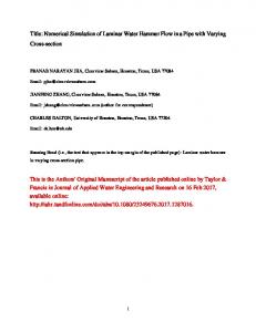
INTRODUCTION A spiral concentrator consists of an open trough that twists downward helically around a central axis. Majority of current designs of spirals have 5 to 7 turns. It is basically a helical sluice, as shown in Fig. (1) Spiral separator is firstly designed and developed based on experience and through many testing of prototypes and modifications. Because of the simplicity of operation and low cost, spirals have been widely used in the mineral industry to separate high-density particles from low-density ones. Development of any spiral design remains largely a process of trial and error. To reduce development time and costs, many experimental models of the spiral were made. Traditionally a spiral separator has been used effectively in the coal and beach sand industries. Currently, it is successfully used to beneficiate a number of ores such as chromite, rutile, gold ore, iron ore, mainly due to its operational simplicity and cost effectiveness. Recently, there has been an accelerated growth in the use of spirals for iron ore beneficiation. The demand for higher efficiency of separation is compromised by a higher capacity in the size range of 3 mm to 45 μm. For iron ore beneficiation, this size range is considered coarse to be treated by floatation and it is considered fine for other conventional gravity separators like jig which performs better for feed materials above 2 mm size. Despite all its advantages, there has been an increased demand to design spirals to accommodate feed materials that vary oversize as well as grade. So, the challenge has been to design the correct profile of the spiral. Since its inception, a lot of work has been done to understand and improve the performance of spirals (Mishra and Tripathy, 2010; Holland-Batt,1995; Machunter et al., 2003; Gulsoy and Kademli,2006; Jancar et al. 1995), However, to predict the performance of a spiral for any given application, and more importantly, to design spirals for a particular ore type to obtain a desired grade, a lot of experiments must be done. These are quite cumbersome and costly. Hence, there are many options in the simulation of the separation process in spiral separators.

in the development of a  mechanistic model of the spiral operation. The model determines the flow fields for simplified rectangular spiral sections. Jancar et al (1995) investigated the fluid flow on LD9 spiral using their developed code. All these models were developed with time to be more reliable. Mathews et al. (1998a,1998b,1999a,1999b) presented CFD modeling of the fluid flow on spiral trough. Doheim et al.(2013) suggested CFD model based on Eulerian approach and turbulence model in case of low solid concentration from 0.3 to 3% solids by weight. The present paper followsthe overall CFD modeling fluid-particle flow in gravity concentrators in spiral separators. The discussions are concentrated on the adoption of realistic solid percent in spiral separatorsof multiphase flow models as well as model validation against experimental data.The present study suggests a particulate-flow computational model based on Eulerian approach. The present model is validated using the experimental data of LD9 spiral (Holland-Batt and Holtham,1991; Holtham,1997; Holtham, 1992). The main objective of this study is to obtain a comprehensive mathematical model according to Computational Fluid Dynamics (CFD). The present study will focus on the shortcomings of the previous mathematical models so as to obtain a more accurate and reliable model.

SPIRAL SEPARATOR DESCRIPTION Spiral Geometry The design parameters of the spiral separator can be listed as: spiral pitch (u), profile shape, length (L), and inner and outer trough radii (ri , ro) that govern the curvature (y) of the channel. The parameters are shown in Fig. (2) and defined as follows (Doheim et al.,2013): Pitch: u = 2 π r tan ( ) (m) Height loss: h = R r tan ( ) (m) Mainstream distance: L(r)=R r/cos( ) (m) Curvature: y=(ri+ro)/2W (dimensionless) Trough width: W=ro–ri (m) Spiral height: H=n*u (m) Where, R is the angular distance in radians in the mainstream direction from the spiral inlet (=2  π  , on full turn), r is the radial distance from the centerline axis, is the descent angle, H is the spiral height and W is the trough width. The geometrical parameters for LD9 spiral are stated in Table 1 (Doheim et al.,2013).

a

a

a

a

Fig. (1) A Humphreys spiral.

Mathematical models are therefore of great value for determining how such flows are influenced by fluid properties and geometrical parameters and, hence, for predicting and improving the performance of these separators (Stokes et al.,2004; Ferziger and Peric, 1999; Loveday and Cilliers,1994; Kuang et al, 2014; Radman et al,2014). These models started by Burch (1962) when he assumed the pulp to be a liquid of uniform viscosity. He also assumed that the secondary flow would not affect the primary flow. Wang and Andrews (1994) introduced a first step

224

Fig. (2) Schematic drawing of a spiral separator.

AFINIDAD LXXII, 571, Julio - Septiembre 2015

The momentum equations two phases (“fluid and ora“w “ The momentum equations for phases (“fluid and particulate” or The solid-phase stresses represent a multi-fluid granular model to3.1.2. describe the behavior offor atwo fluid-solid mixture. MOMENTUM EQUATIONS represent a multi-fluid granular model to describe flow behavior of a model fluid-solid mixture. represent a multi-fluid granular model togranular describe the flow behavior of aparticulate” fluid-solid mixt represent a the multi-fluid granular model to the flow behavior of represent aflow multi-fluid todescribe describe the flow behavior of fa represent a multi-fluid granular model to describe the flow behavior of a fl The solid-phase stresses are derived by making an analo MOMENTUM (liquid (water, 𝒍𝒍) ) and particulate represent a multi-fluid granular model to describe 3.1.2. the flow behavior ofEQUATIONS a fluid-solid mixture. (solids, 𝒔𝒔) are: represent aare multi-fluid granular model todescribe describe the flow behavior of f represent multi-fluid model to the flow behavior of a aflu momentum equations for two phases (“fluid and particulate” or “water and arising from particle-part TheThe solid-phase stresses are derived byThe making ana an analogy of granular the random particle motions solid-phase stresses are derived by making analogy of the particle motions The solid-phase stresses derived by making an analogy of an the random particle moti The solid-phase stresses are derived by of thethe random The solid-phase stresses arerandom derived bymaking making ananalogy analogy of rand Themomentum solid-phaseequations stresses aretwo derived by(“fluid making anparticulate” analogy of the random The for phases and or “water and arising from particle-particle collisions. The momentum c N The solid-phase stresses are derived by making an analogy∂of the random particle motions  derived  to   of represent a multi-fluid granular model the⋅τfluid flow behavior fluid-solid The solid-phase stresses are making an analogy the)R rando The solid-phase derived making an(liquid ofofathe random ρcollisions. αbylby αanalogy (α lparticle-particle ) = −describe vstresses vequations pThe Fconservation + ∇ ⋅ (αare ∇ +conservation ∇ +(water, arising from particle-particle collisions. The momentum equations for the and pa arising from particle-particle collisions. The momentum for the arising from particle-particle The fl arising from collisions. momentum conservation equa arising from particle-particle The momentum eq lconservation l )conservation l ρl v l momentum lcollisions. l +fluid l ρ l gequations lift ,l + 𝒍𝒍)for slthe represent a∂multi-fluid granular model to describe the flow behavior of a fluid-solid t particle-particle arising from collisions. The momentum conservation equa 1 l = (liquid (water, 𝒍𝒍)the ) and particulate (solids, 𝒔𝒔) are: arising from particle-particle collisions. The momentum conservation equations for fluid The solid-phase stresses are derived by making anmomentum analogy of theconservation random particle arising fromparticle-particle particle-particle collisions. The momentum equ arising from The equat (liquid (water, 𝒍𝒍) )𝒍𝒍)and particulate (solids, 𝒔𝒔) (liquid (water, ) and particulate (solids, 𝒔𝒔) are: (liquid (water, 𝒍𝒍) )are: and particulate 𝒔𝒔)collisions. are:by(solids, (liquid (water, 𝒍𝒍) 𝒍𝒍) ) and particulate 𝒔𝒔)an are: (liquid (water, )(solids, and particulate (solids, 𝒔𝒔) are: ∂ of conservation  random particle N  The solid-phase stresses are derived making analogy the  (liquid (water, 𝒍𝒍) ) and particulate (solids, 𝒔𝒔) are: α ρ α ρ ( ) ( v v + ∇ ⋅ ∂ l l l equations l v l N)t  ρ v v ) =The ∇  p − ∇p + ∇ F l +l for (liquid (water, 𝒍𝒍) ) and particulate (solids, 𝒔𝒔) are: arising from∂ particle-particle collisions. momentum conservation t ∂ + ∇ ⋅ − ⋅ + + v g ( ) ( α ρ α α τ α ρ (liquid (water, 𝒍𝒍) and particulate (solids, 𝒔𝒔) are: (liquid (water, 𝒍𝒍) ) and particulate (solids, 𝒔𝒔) are: α ρ α ρ α τ α ρ ( ) ( ) v v v p g F + ∇ ⋅ = − ∇ + ∇ ⋅ + + +R s s s s s s s s s s s s lift s , an analogy of the random particle motions arising from Table (1) The geometrical parameters of LD9 N N N N l l l l lift ,l for  l l momentum   l N l equations    ∂ ∂ ∂   arising   ∂t particle-particle  l The l  l collisions.  conservation ∂ ∂ from l =1 l = t ∂ N (α (ρα vρet )v+al.,2013 (α⋅l(ραl lvρl vl vl )l v=l )−=α(−lα∇αl pρl ∇+l vp∇l +)⋅+τ∇l∇ +τ⋅∂α collisions. The spiral separator (Doheim )∇+⋅ ∇ F,l)−lift ⋅particle-particle +l (lρααρl(water, )+lift Rρconservation +llRρv∇lsllv⋅τll )vl l=+) α α⋅ (Rpαρparticulate α+lα(2) )v=+l𝒍𝒍) p∇++pF∇ ∇+)α,l⋅and −=α(solids, (llgαρNvρ+lllvgρvF ∇(+∇ −ρα∇l glmomentum + ⋅∇τare: ⋅+τ+(2) (2) gl +g F+liftF,lift sl 𝒔𝒔) l(α l + ,l + R slR sl lsll ρ  ∂t ∂t l l l l l l   (liquid ∂ ρ lvRllll)for ρ=1lparticulate ) = −αl ll(water, +∇ ⋅ (l=α1 lllfluid ∇p + ∇lift⋅τl),lll )+lα + F∂lift  ,l + Nl =N1 lR=1sl l =1l ρ l g  particulate v lv l(liquid ρ l v l v l ) =Descent (α l ρ l v l ) + ∇ F∂∂lift∂t∂t,l∂(α+(tαl (water, ⋅ (α lCurva−α l ∇p +Number ∇∂⋅tτ l + α l ρ l g + equations (liquid 𝒍𝒍) the ) land (solids, 𝒔𝒔) are:and (2) 𝒕𝒕𝒕𝒕 Outer Trough Inner sl + ∇ ⋅ (α s ρs vs vs) αl ∇l ∇ ) +∇∇⋅ (α vvllv)l 𝒒𝒒 g+ +FN lift Flift,(lα,+l s +ρl s=v1 Rs )R ⋅𝝉𝝉�(αl𝒒𝒒∂ρlislρvllthe ∇⋅τ⋅lτ+l +ααl ρl lρgltensor. stress-strain (α l ρll=lρ1s) vWhere: p p+ +∇ =) =−α−phase Pitch llv)are: l+ sl sl  (solids, of Turns Radius Radius ∂tWidth angle ture    ∂ ∂t ∂t(∂αtl ρ l v l ) + ∇ ⋅ (α l ρ l vl v l(α =1 ⋅τ + α ρ g + F u (mm) =1l ∇ N ρ v ) + ∇ ⋅ (α ρ v v ) = −α ∇p N−R∇p s l+ (2 l n ri(mm) ro (mm) W (mm) α( o )   ∂ ∂ ∂  y  sl    s NN N s s ∂ ∂     ∂t ) =s −sαNls∇p + ∇ ⋅τ l s+ αs lsρ lsg+ Flift ,ls +N∑ ∂t∂∇ 1ρ R l =α 𝟐𝟐 + ⋅ + + + p g F R (α s(ραssvρs )s v+s )∇+⋅ ∇ (α⋅s(ραssvρs vs vs )s v=s )−=α(−sα∇αspρs ∇−s vp∇ τ α ρ (3) − ∇ + ∇ ⋅ + + + p g F R τ α ρ + ∇ ⋅ = − ∇ − ∇ + ∇ ⋅ + + + v v p p g F R ) ( ) α ρ α τ α ρ + ∇ ⋅ = − ∇ − ∇ + ∇ ⋅ + + + v v v p p g F R ( ) ( ) α ρ α ρ α τ α α ρ α ρ α τ α ρ ( ) ( ) v v v p g F + ∇ ⋅ = − + ⋅ + + + + ∇ ⋅ = − ∇ − ∇ + ∇ ⋅ + + + v v p p g F R ( ) ( ) α ρ α ρ α τ ρ (3) (3)   ( s sss sssN s l sliftl , sslift lss l ls �⃗𝑻𝑻 ,sls �ss⃗ ∑ s s s ∂ s sl sl s slss𝝉𝝉 s �s +ls𝜶𝜶s l�𝝀𝝀 lss  �𝒗𝒗 , s slift𝝁𝝁 ,ls � l �𝛁𝛁𝒗𝒗 ls lift sls⃗ 𝑰𝑰 � s s s s lift s ls , s s s lift s ls , = 𝜶𝜶 𝝁𝝁 + 𝛁𝛁𝒗𝒗 − 𝛁𝛁. � 70 350   7 - 32 ∂ 280  ∂t273 𝒒𝒒 ⋅τ 𝟑𝟑+ α𝒒𝒒 Where: 𝒒𝒒 (2) N 𝒒𝒒𝒕𝒕𝒕𝒕 phas ∂t∂∂t ∂(αt s ρ svs𝒒𝒒) + ∇ ⋅ 𝒒𝒒(α s𝒒𝒒ρ svls=v1 𝒒𝒒sl)=1= −α s𝒒𝒒∇p − ∇p𝒒𝒒 s + ∇ ∂t⋅ (α ρ0.75 ∂6t =1s g+  l =1s lρ =1 lR s =1ls  NFlift𝝉𝝉�,𝒒𝒒s +isNlthe +(αFliftρ,s v+) + ∇Rls⋅ (α ρ v v ) = −α ∇(3) (α s ρ s vs ) + ∇ s s vs vs ) = −α s ∇p − ∇p s + ∇ ⋅τ s + α s ρ∂ sg ∂ t 𝒕𝒕𝒕𝒕 − ∇ + ∇ ⋅ + + + p p g F R τ α ρ l = 1  ∇s p −𝒒𝒒∇pphase +s ∇ ⋅τstress-strain +s α s ρs s gs + Ftensor. Rls ls α the ρss vss ss )s𝝉𝝉�=𝒒𝒒−is ∂ (α s ρs s vss )s+l =∇1 ⋅ (αWhere: s ∂t liftlift , s ,+ + ∇ ⋅ (α s ρ𝝁𝝁s vs s v𝒕𝒕𝒕𝒕 = −𝝀𝝀α s ∇ ∇psshear + ∇ ⋅sτ sand + α sbulk p −sthe Flift ρ s vs )Where, ρss g +viscosity (3 ∂t(∂αts 𝒕𝒕𝒕𝒕 s )𝒕𝒕𝒕𝒕 ls phase Mechanism of Particle Separation l =1l =1 q, 𝑭𝑭  ,s + ∑N Rof 𝒕𝒕𝒕𝒕 and are  𝝉𝝉�𝒒𝒒𝝉𝝉�is    Where: 𝝉𝝉�𝒒𝒒 𝝉𝝉�is𝒒𝒒 the 𝒒𝒒𝒕𝒕𝒕𝒕𝒒𝒒phase stress-strain 𝒒𝒒 𝒒𝒒 𝑳𝑳𝑳𝑳𝑳𝑳𝑳𝑳 Where: is the phase stress-strain tensor. 𝑻𝑻 Where: 𝝉𝝉�𝒒𝒒 istensor. the 𝒒𝒒 phase stress-strain tensor. ∂t∂Where: the 𝒒𝒒 phase stress-strain tensor. Where: is the 𝒒𝒒 phase stress-strain tensor. l = 1 𝒒𝒒⋅ (α ρ v𝒕𝒕𝒕𝒕v ) = −α ∇p − ∇p + ∇ ⋅τ + α ρ g + F � ⃗ � ⃗ = 𝜶𝜶 𝝁𝝁 �𝛁𝛁𝒗𝒗 + 𝛁𝛁𝒗𝒗 � 𝝉𝝉 � + ∇ + v R ( ) α ρ ( 𝒒𝒒 𝒒𝒒 𝒒𝒒 𝒒𝒒 𝒒𝒒 ∑ s s s s s s s s s s s s lift s ls , Feed is introduced through the feed box at the top of spi(3) 𝝉𝝉�𝒒𝒒 is the 𝒒𝒒 phase stress-strain tensor. 𝟐𝟐 𝑻𝑻 ∂Where: t Where: 𝝉𝝉� is the 𝒒𝒒𝒕𝒕𝒕𝒕 phase stress-strain tensor. =1 � 𝛁𝛁. � 𝒕𝒕𝒕𝒕 �⃗𝒒𝒒 + 𝛁𝛁𝒗𝒗 �⃗tensor. = 𝜶𝜶𝒒𝒒 𝝁𝝁stress-strain �𝛁𝛁𝒗𝒗 �+ 𝜶𝜶𝒒𝒒 �𝝀𝝀𝒒𝒒 − 𝟑𝟑 l𝝁𝝁 𝒗𝒗⃗𝒒𝒒 𝑰𝑰� 𝝉𝝉�𝒒𝒒 𝒕𝒕𝒕𝒕 𝒒𝒒 𝒒𝒒 𝒒𝒒 𝒒𝒒 Where: 𝝉𝝉 � is the phase stress-strain tensor. ral, which establishes the 𝒒𝒒correct pattern of the𝑻𝑻flow. The Where: is the phase stress-strain tensor. Where: 𝝉𝝉 � is the 𝒒𝒒 phase 𝒕𝒕𝒕𝒕 𝟐𝟐 Where: 𝒒𝒒 𝒒𝒒the 𝒒𝒒 shared 𝟐𝟐by phases,𝒗𝒗 𝟐𝟐𝒒𝒒 𝟐𝟐is velocity of phase velocity of pha 𝝉𝝉�𝒒𝒒𝑰𝑰��𝒗𝒗⃗𝑻𝑻pressure phase 𝑻𝑻stress-strain 𝑻𝑻+all ⃗𝒒𝒒 �+ �𝒗𝒗𝛁𝛁𝒗𝒗 ⃗= =𝒒𝒒 𝜶𝜶 𝝁𝝁𝒒𝒒 𝝁𝝁 �𝛁𝛁𝒗𝒗 𝝁𝝁𝟐𝟐𝒒𝒒�⃗𝝁𝝁 �𝝉𝝉𝒒𝒒𝒒𝒒𝒒𝒒𝛁𝛁. 𝝉𝝉�𝒒𝒒 𝝉𝝉�as ⃗𝒒𝒒 𝛁𝛁𝒗𝒗 �⃗𝑻𝑻𝒒𝒒+�𝝉𝝉�𝜶𝜶 = 𝜶𝜶 +�⃗𝛁𝛁𝒗𝒗 + 𝜶𝜶�𝝀𝝀 �𝝀𝝀 �= (4) �𝒗𝒗𝒒𝒒⃗𝒒𝒒�𝝀𝝀 𝝁𝝁𝒒𝒒𝒒𝒒𝟑𝟑− �𝛁𝛁𝒗𝒗 �𝒒𝒒𝑰𝑰�𝒒𝒒𝝁𝝁 +�𝛁𝛁𝒗𝒗 −�𝛁𝛁𝒗𝒗 𝑰𝑰�tensor. �⃗𝒒𝒒𝒒𝒒𝒕𝒕𝒕𝒕��𝝀𝝀 ⃗𝑻𝑻𝒒𝒒𝟑𝟑�⃗�𝝁𝝁 �𝒗𝒗⃗𝒒𝒒�𝒗𝒗⃗𝑰𝑰�𝒒𝒒Where, 𝜶𝜶�⃗𝒒𝒒𝒒𝒒𝜶𝜶is 𝛁𝛁𝒗𝒗 𝜶𝜶𝛁𝛁.𝒒𝒒𝜶𝜶�𝝀𝝀 − ⃗+ 𝝉𝝉�+ �𝛁𝛁𝒗𝒗 𝝁𝝁�𝒒𝒒𝛁𝛁. � 𝛁𝛁. 𝑰𝑰� 𝒒𝒒 � 𝒒𝒒= 𝒒𝒒 𝒒𝒒 ��𝛁𝛁𝒗𝒗 𝒒𝒒𝜶𝜶𝒒𝒒 𝒒𝒒𝝁𝝁 𝟐𝟐𝟑𝟑 𝝁𝝁 𝒒𝒒The 𝒒𝒒− 𝒒𝒒 �+ 𝒒𝒒 𝒒𝒒(4) are the 𝒒𝒒𝛁𝛁. 𝒒𝒒𝜶𝜶 𝒒𝒒 𝒒𝒒+ 𝒒𝒒 � 𝒒𝒒 − feed enters the spiral trough a 𝒒𝒒homogenous slurry. (4)𝝁𝝁𝒒𝒒 and 𝝀𝝀𝒒𝒒 (4) 𝟑𝟑Where: 𝝉𝝉 � is the 𝒒𝒒 phase stress-strain tensor. 𝟐𝟐 � ⃗ � ⃗ = 𝜶𝜶 𝝁𝝁 �𝛁𝛁𝒗𝒗 + 𝛁𝛁𝒗𝒗 � + 𝜶𝜶 �𝝀𝝀 − 𝝁𝝁𝟑𝟑𝒒𝒒 � 𝛁𝛁. �𝒗𝒗⃗𝒒𝒒 𝑰𝑰� 𝝉𝝉 � 𝒒𝒒 𝑻𝑻 𝒒𝒒 𝒒𝒒 𝒒𝒒 𝒒𝒒 𝒒𝒒 𝒒𝒒 𝒒𝒒 = − R k ( v v ) � 𝟐𝟐 sl sl s l � ⃗ � ⃗ � ⃗ 𝟑𝟑 = 𝜶𝜶 𝝁𝝁 �𝛁𝛁𝒗𝒗 + 𝛁𝛁𝒗𝒗 � + 𝜶𝜶 �𝝀𝝀 − 𝝁𝝁 � 𝛁𝛁. 𝒗𝒗 𝑰𝑰 (4) 𝝉𝝉 � 𝟐𝟐 Where, 𝝁𝝁 and 𝝀𝝀 are the shear and bulk viscosity of phase 𝒒𝒒 𝒒𝒒 𝒒𝒒 spiral 𝒒𝒒 separates 𝒒𝒒 𝒒𝒒 miner𝒒𝒒 𝟐𝟐 𝒒𝒒 − 𝝁𝝁 � 𝛁𝛁. 𝒗𝒗 pulp flows spirally𝒒𝒒downward, the 𝑻𝑻⃗𝑻𝑻 � + 𝒒𝒒 � 𝑻𝑻 � 𝟑𝟑 𝒒𝒒 � ⃗ � � ⃗ = 𝜶𝜶 𝝁𝝁 �𝛁𝛁𝒗𝒗 + 𝛁𝛁𝒗𝒗 𝜶𝜶 �𝝀𝝀 𝑰𝑰 𝝉𝝉 � � particulate phase), 𝒗𝒗 is velocity of liquid phase, 𝒗𝒗 is velocity of(4s ⃗𝒒𝒒 𝛁𝛁𝒗𝒗 𝜶𝜶𝒍𝒍𝒒𝒒𝒒𝒒 − �𝝀𝝀𝒒𝒒𝝁𝝁𝒒𝒒− 𝝁𝝁 �𝒒𝒒 𝒒𝒒=𝒒𝒒=𝜶𝜶𝒒𝒒𝜶𝜶𝝁𝝁𝒒𝒒𝒒𝒒𝝁𝝁 𝒒𝒒�𝛁𝛁𝒗𝒗 𝒒𝒒 𝒒𝒒+ 𝒒𝒒 �⃗𝒒𝒒�+ �⃗𝒒𝒒𝛁𝛁𝒗𝒗 �𝒒𝒒⃗𝒒𝒒�𝒒𝒒𝑰𝑰𝛁𝛁. �𝒗𝒗⃗𝒒𝒒 𝑰𝑰𝒒𝒒 ��⃗+𝒒𝒒 �𝒒𝒒𝜶𝜶+ 𝝉𝝉�𝝉𝝉 𝒔𝒔 𝒒𝒒 �𝛁𝛁𝒗𝒗 𝒒𝒒 �𝝀𝝀 𝒒𝒒 �𝟑𝟑𝛁𝛁. 𝟑𝟑 𝒗𝒗 𝟑𝟑𝟐𝟐lift Where, 𝝁𝝁𝒒𝒒 𝝁𝝁and 𝝀𝝀𝒒𝒒 𝝀𝝀are thethe shear andand viscosity phase 𝑭𝑭are is,𝒒𝒒 aisshear lift force, pviscosity is�viscosity the Where, and are shear bulk of phase 𝑭𝑭𝑳𝑳𝑳𝑳𝑳𝑳𝑳𝑳 aand force, pq, is 𝑭𝑭viscosity the Where, 𝝁𝝁bulk 𝝀𝝀viscosity are the bulk viscosity of phase isphase a of lift pisall isis Where, 𝝁𝝁of𝒒𝒒𝝁𝝁shear and 𝝀𝝀and the shear bulk of,𝒒𝒒of phase q,force, 𝑭𝑭𝑳𝑳𝑳𝑳𝑳𝑳𝑳𝑳 athe lif als in accordance with their specific particle Where, are and bulk and 𝝀𝝀�⃗are the shear and bulk q, 𝑭𝑭𝑳𝑳𝑳𝑳𝑳𝑳𝑳𝑳 al pressure shared by pha 𝑳𝑳𝑳𝑳𝑳𝑳𝑳𝑳 ,𝒒𝒒the 𝒒𝒒gravity 𝒒𝒒and 𝒒𝒒 and 𝒒𝒒Where, 𝑳𝑳𝑳𝑳𝑳𝑳𝑳𝑳 𝒒𝒒q, ,𝒒𝒒 𝒒𝒒⃗and 𝒒𝒒𝑻𝑻q, ,𝒒𝒒 � � ⃗ = 𝜶𝜶 𝝁𝝁 �𝛁𝛁𝒗𝒗 + 𝛁𝛁𝒗𝒗 � + 𝜶𝜶 �𝝀𝝀 − 𝝁𝝁 � 𝛁𝛁. 𝒗𝒗 𝑰𝑰 𝝉𝝉�Where, 𝒒𝒒 𝒒𝒒 𝝁𝝁 𝒒𝒒 𝒒𝒒 and 𝒒𝒒 𝝀𝝀𝒒𝒒 are 𝒒𝒒 the shear 𝒒𝒒 𝒒𝒒 and 𝒒𝒒 𝒒𝒒 bulk viscosity ofvelocity phase q,of𝑭𝑭phase a lift(4 (5) 𝑳𝑳𝑳𝑳𝑳𝑳𝑳𝑳 ,𝒒𝒒 isveloci 𝟑𝟑 the pressure shared by all phases,𝒗𝒗 is size. Low densityWhere, and small size𝝀𝝀particles remain suspendphase q, a lift force, p is the pressure shared 𝝁𝝁𝒒𝒒 and are the shear and bulk viscosity of phase q, 𝑭𝑭 is a lift force, p is 𝒒𝒒 𝒒𝒒 𝑳𝑳𝑳𝑳𝑳𝑳𝑳𝑳 ,𝒒𝒒𝝀𝝀  Where, is interaction force between phases. 𝝀𝝀𝒒𝒒an the shear and bulk viscosity of phase q,phase 𝑭𝑭𝑳𝑳𝑳𝑳𝑳𝑳𝑳𝑳 q, is𝑭𝑭a𝑭𝑭 lift force, plif is 𝝁𝝁𝒒𝒒𝝁𝝁𝑹𝑹and 𝒍𝒍𝒍𝒍and Where, 𝝁𝝁 and arethe theshear shear and bulkviscosity viscosity of phase Where, 𝝀𝝀are are and bulk ofphase isisa alift ,𝒒𝒒q, 𝑳𝑳𝑳𝑳𝑳𝑳𝑳𝑳 ,𝒒𝒒 𝒒𝒒shared 𝒒𝒒 𝑳𝑳𝑳𝑳𝑳𝑳𝑳𝑳 ,𝒒𝒒 pressure by by allforce phases,𝒗𝒗 of of phase qof (liquid or solided and travel outwards due to the shared centrifugal to acby all(phase of phase velocity of q of pressure shared all phases,𝒗𝒗 isshared of phase of phase q𝒒𝒒bulk (liquid or solidpressure all phases,𝒗𝒗 velocity phase velocity of phase q (liquid or solidpressure by𝒒𝒒is all phases,𝒗𝒗 is velocity of phase velocity phase particulate phase), 𝒗𝒗q𝒍𝒍 (liq velocity of phase velocity of phase qisp(lvi pressure shared by all phases,𝒗𝒗 𝒒𝒒 is𝒒𝒒 velocity ) 𝝀𝝀velocity Rvelocity kby vphases, v𝒒𝒒svelocity 𝒒𝒒 𝒒𝒒 is ls = ls l𝝁𝝁− and are the shear and viscosity of phase q, 𝑭𝑭 is a lift force, Where, 𝒒𝒒 𝒒𝒒 𝑳𝑳𝑳𝑳𝑳𝑳𝑳𝑳 ,𝒒𝒒 pressure shared by all phases,𝒗𝒗 of phase of phase q (liq 𝒒𝒒 is velocity cumulate in the outer trough regions, whilst high density of phase (liquid or solid-particulate velocity liquid particulate phase), 𝒗𝒗𝒍𝒍ofisis velocity ofofvelocity liquid phase, 𝒗𝒗𝒔𝒔 or is velo pressure shared by all phases,𝒗𝒗 velocity of phase qphases,𝒗𝒗 or solid (liquid𝒒𝒒phase), 𝒒𝒒 is velocity is isisvelocity pressure shared by by allby velocity phase velocity of phase soli pressure shared phases,𝒗𝒗 phasevelocity velocity phase q(liqu (liq pressure shared allslallphases,𝒗𝒗 of𝑹𝑹of phase ofqof(liquid phase qforce 𝒒𝒒 ) velocity = − R k ( v v 𝒒𝒒phase, particulate is velocity of liquid phase, 𝒗𝒗 is velocity of solid phase, and 𝑹𝑹 or and coarse size particles settle in thephase), flow to𝒗𝒗slide inwards phase, velocity of solid and or is an sl s l is an interaction 𝑹𝑹 is velocity of liquid phase, 𝒗𝒗 is velocity of solid phase, and or particulate phase), 𝒗𝒗 particulate phase), 𝒗𝒗 is velocity of liquid phase, 𝒗𝒗 is velocity of solid phase, and 𝑹𝑹 or particulate phase), 𝒗𝒗 is velocity of liquid phase, 𝒗𝒗 is velocity of solid particulate phase), 𝒗𝒗 is velocity of liquid phase, 𝒗𝒗 is velocity of solid p 𝒍𝒍 𝒍𝒍 𝒔𝒔𝒔𝒔𝑲𝑲𝒔𝒔𝒔𝒔velocity 𝒍𝒍𝒍𝒍𝒔𝒔)of 𝒔𝒔 by all phases,𝒗𝒗 𝒍𝒍 shared 𝒔𝒔phases, 𝒍𝒍 force 𝒔𝒔𝒍𝒍𝒍𝒍 pressure is velocity of phase phase q (liquid 𝒔𝒔𝒔𝒔orpha sol 𝒍𝒍 Where,𝑹𝑹 an𝒔𝒔 interaction is the momentum-exc 𝒒𝒒between 𝒔𝒔𝒔𝒔is 𝒔𝒔𝒔𝒔 (=𝑲𝑲 particulate phase), 𝒗𝒗 is velocity of liquid phase, 𝒗𝒗 is velocity of solid pha   𝒍𝒍is 𝒔𝒔phases. an interaction force between 𝑹𝑹 toward the central column (Fig. 3). 𝒗𝒗𝒍𝒍 is velocity of liquid phase, 𝒗𝒗particulate interaction force between phases. Equations (2 & 3) must be closed with appropriate expressions for t𝒔𝒔 𝒍𝒍𝒍𝒍 phase), 𝒗𝒗 is velocity of liquid phase, 𝒗𝒗 is velocity of solid phase, and 𝑹𝑹 particulate phase), is velocity of solid phase, and 𝑹𝑹 or 𝒔𝒔 𝒔𝒔  𝒔𝒔𝒔𝒔of liquid phase, Rsl = kphase), (vs −𝒍𝒍 𝒗𝒗 vl𝒗𝒗)𝒍𝒍isisvelocity particulate velocity 𝒗𝒗 velocityofofsolid solidphas pha slphase), particulate of liquid phase, 𝒗𝒗velocity isisvelocity 𝒍𝒍phases. 𝒔𝒔 𝒔𝒔expresinteraction force between 𝑹𝑹𝒍𝒍𝒍𝒍𝑹𝑹is𝒍𝒍𝒍𝒍an Equations must besolid”] closed with appropriate is an interaction force phases. interaction force between 𝑹𝑹between 𝑹𝑹 an force between phases. 𝑹𝑹is is interaction force between phases. particulate phase), 𝒗𝒗 is velocity of liquid phase, 𝒗𝒗 is of solid phase, and 𝑹𝑹 = − Rsl𝒍𝒍𝒍𝒍 k slan (interaction v(2 & 3) v ) 𝒍𝒍𝒍𝒍 is anphases.  𝒍𝒍𝒍𝒍 𝒍𝒍 𝒔𝒔 N is the tota coefficient between fluid [not “or phase (l) and solid phase (s), and s l   Rforce an between 𝑹𝑹 (vl phases. on 𝒍𝒍𝒍𝒍 is anfor interaction force between 𝑹𝑹sions k(lsforce v)s )phases. the inter-phase depends on cohesion the theforce friction, pressure, and other 𝑅𝑅interaction 𝒍𝒍𝒍𝒍 is 𝑹𝑹𝒍𝒍𝒍𝒍 is an interaction force between phases. ls = 𝑠𝑠𝑠𝑠 .This = −−v.This Rforce kdepends vbetween is an interaction force phases. 𝑹𝑹 sl sl s l is an interaction force between phases. 𝑹𝑹 𝒍𝒍𝒍𝒍 𝒍𝒍𝒍𝒍 Equations (2 & 3)(5) must b  force between phases. 𝑹𝑹𝒍𝒍𝒍𝒍 is an interaction friction, pressure, cohesion and other effects, and is sub  phases. (vs − vl ) Rsl(v= − kEquations  to sl kconditions (2 &=interaction 3) must be𝑹𝑹 closed with appropriate expressi 𝒔𝒔𝒔𝒔an = ) R v ject the that Where,𝑹𝑹 is force between phases, 𝑲𝑲 (=𝑲𝑲 the conditions that 𝑹𝑹 𝑹𝑹 and = 𝟎𝟎. 𝒔𝒔𝒔𝒔 𝒔𝒔𝒔𝒔 𝒍𝒍𝒍𝒍 ) is t ls ls l s 𝒍𝒍𝒍𝒍 𝒍𝒍𝒍𝒍 Rls = kls (expressions v − vs ) Rslfor = kthe vinter-phase vl ) sl (the s −inter-phase Equations (2 & be be closed with force .This forcefordepends on Equations (2 3) & must 3) must closed appropriate expressions for force for𝑅𝑅expressions Equations (2appropriate & 3)Equations must bel(2 closed with appropriate expressions the inter-phase force Equations & 3) must be closed with appropriate the inter(2 & 3) must be closed with appropriate for the inte 𝑠𝑠𝑠𝑠expressions The simple interaction term is:  � ⃗ � ⃗ � ⃗ = −𝟎𝟎. 𝟓𝟓𝝆𝝆 𝜶𝜶 �𝒗𝒗 − 𝒗𝒗 � × (𝛁𝛁 × 𝒗𝒗 ) (6) 𝑭𝑭with   (2 & 3) must be closed with appropriate expressions for the inter-phase forc 𝒍𝒍𝒍𝒍𝒍𝒍𝒍𝒍Equations 𝒒𝒒 𝒑𝒑 𝒒𝒒 𝒑𝒑 𝒒𝒒 Equations (2 simple & 3) must be(force closed with appropriate expressions thephase inter= between fluid [not solid”] phase (l) andfor solid (sa 𝑅𝑅coefficient .This depends on “or thephases, friction, pressure, cohesion   𝑠𝑠𝑠𝑠 − ) R k v v The interaction term is: Equations (2 & 3) must be closed with appropriate expressions for the inter-phase force  Where,𝑹𝑹 is an interaction force between 𝑲𝑲 (=𝑲𝑲 ) is the mome   ls k 𝒔𝒔𝒔𝒔 𝒔𝒔𝒔𝒔for 𝒍𝒍𝒍𝒍inter-phase Equations & must be=be closed with appropriate expressions for Where,𝑹𝑹 isR an interaction force between phases, 𝑲𝑲𝒔𝒔𝒔𝒔to (=𝑲𝑲 is thethe momentum-exchan Equations (2 3)lsmust must be appropriate expressions for the𝑹𝑹 inter R (lclosed veffects, )with −svwith Equations &3)& 3) appropriate expressions for the inter-p 𝒔𝒔𝒔𝒔(2(2 𝒍𝒍𝒍𝒍 )conditions sl − slclosed s friction, land  𝑅𝑅𝑠𝑠𝑠𝑠𝑅𝑅.This force depends on the friction, pressure, cohesion and other effects, is subject = ( ) k v v = the that .This force depends on the friction, pressure, cohesion and other and is subject to 𝑅𝑅 .This force depends on the friction, pressure, cohesion and other effects, and is subject  .This force depends on the pressure, cohesion and other effects, 𝑅𝑅 .This force depends on the friction, pressure, cohesion and other effect 𝑅𝑅   ls ls onl the sfriction, 𝑠𝑠𝑠𝑠 𝑠𝑠𝑠𝑠 𝑠𝑠𝑠𝑠 𝑠𝑠𝑠𝑠 force depends  pressure, cohesion and other effects, and is𝒔𝒔𝒔𝒔subjt =𝑅𝑅𝑠𝑠𝑠𝑠𝑅𝑅k.This − force (vsand vother phases. depends pressure, cohesion and other effects, a =on −that (is Rlsconditions klsthe vl friction, vs ) 𝑹𝑹to  𝑠𝑠𝑠𝑠 sl .This l) -cohesion 𝑹𝑹𝒍𝒍𝒍𝒍solid and 𝑹𝑹𝒍𝒍𝒍𝒍solid = 𝟎𝟎.and the  Rslcohesion 6other 𝒔𝒔𝒔𝒔 = pressure, effects, and subject 𝑅𝑅𝑠𝑠𝑠𝑠 .This force depends on the friction, (5) 𝑅𝑅 .This force depends the friction, pressure, and effects, and is N sub coefficient between fluid [not “or solid”] (l)between and phase (s), and N is total coefficient between fluidon[not solid”] phase (l)phase and phase (s), Where,𝑹𝑹 is an interaction force phases, 𝑲𝑲the (=𝑲𝑲 𝑠𝑠𝑠𝑠 𝒔𝒔𝒔𝒔“or 𝒔𝒔𝒔𝒔effects, 𝒍𝒍𝒍𝒍n 𝑅𝑅 .This force depends on the friction, pressure, cohesion and other = − R k ( v v ) 𝑅𝑅 .This force depends on the friction, pressure, cohesion and other effects, a)i 𝑠𝑠𝑠𝑠 𝑠𝑠𝑠𝑠 sl sl s l = 𝑹𝑹 and 𝑹𝑹 = 𝟎𝟎. thethe conditions that 𝑹𝑹 The simple interaction ter Where,𝑹𝑹 is an interaction force between phases, 𝑲𝑲 (=𝑲𝑲 conditions that𝒔𝒔𝒔𝒔𝑹𝑹𝒔𝒔𝒔𝒔 = the -𝒍𝒍𝒍𝒍𝑹𝑹conditions =that 𝟎𝟎. 𝑹𝑹𝒍𝒍𝒍𝒍that and 𝟎𝟎. 𝑹𝑹conditions the conditions 𝑹𝑹 == -and 𝑹𝑹- 𝒍𝒍𝒍𝒍 and == 𝟎𝟎.𝟎𝟎. 𝑹𝑹-𝒔𝒔𝒔𝒔𝑹𝑹 𝑹𝑹𝑹𝑹𝒍𝒍𝒍𝒍 and the that 𝒍𝒍𝒍𝒍𝑹𝑹𝒍𝒍𝒍𝒍the = 𝑹𝑹 𝟎𝟎.𝒍𝒍𝒍𝒍𝑹𝑹𝒍𝒍𝒍𝒍 conditions 𝑹𝑹 𝒔𝒔𝒔𝒔= 𝒔𝒔𝒔𝒔 𝒍𝒍𝒍𝒍 ) is the mome 𝒍𝒍𝒍𝒍 and3.2. 𝒔𝒔𝒔𝒔 = - that 𝒍𝒍𝒍𝒍𝑹𝑹𝒔𝒔𝒔𝒔 𝒔𝒔𝒔𝒔𝑭𝑭 𝒍𝒍𝒍𝒍 = 𝒍𝒍𝒍𝒍  TURBULENCE MODELS � ⃗ � ⃗ � ⃗ = −𝟎𝟎. 𝟓𝟓𝝆𝝆 𝜶𝜶 �𝒗𝒗 − 𝒗𝒗 � × (𝛁𝛁 × 𝒗𝒗 ) 𝒍𝒍𝒍𝒍𝒍𝒍𝒍𝒍 𝒒𝒒 𝒑𝒑 𝒒𝒒 𝒑𝒑 𝒒𝒒 = 𝑹𝑹 and 𝑹𝑹 = 𝟎𝟎. the conditions that 𝑹𝑹 = kls𝒔𝒔𝒔𝒔and −between (𝒍𝒍𝒍𝒍 ) 𝟎𝟎. R𝒔𝒔𝒔𝒔simple visinteraction vinteraction 𝒍𝒍𝒍𝒍 term Where,𝑹𝑹 an force phases, 𝑲𝑲𝒔𝒔𝒔𝒔 (=𝑲𝑲(5) ) is is: between l 𝑹𝑹 phases. the conditions 𝑹𝑹The the conditions that 𝑹𝑹𝒔𝒔𝒔𝒔 = - 𝑹𝑹𝒍𝒍𝒍𝒍 and 𝑹𝑹𝒍𝒍𝒍𝒍 = 𝟎𝟎.  Where, is anthat interaction phases, (=) is the 𝒔𝒔𝒔𝒔 =ls- 𝑹𝑹𝒍𝒍𝒍𝒍force 𝒍𝒍𝒍𝒍 s= phases. coefficient between fluid [not solid”] phase (l) and solid𝒍𝒍𝒍𝒍phas =- 𝑹𝑹 - 𝑹𝑹 and 𝑹𝑹 =𝟎𝟎. 𝟎𝟎.“or the conditions that 𝑹𝑹 simple 𝑹𝑹 the conditions that 𝑹𝑹term 𝒍𝒍𝒍𝒍and coefficient between fluid [not “or phase (l) and (5) solid phase (s), and N i 𝒔𝒔𝒔𝒔𝒔𝒔𝒔𝒔=term 𝒍𝒍𝒍𝒍is: 𝒍𝒍𝒍𝒍 𝒍𝒍𝒍𝒍=solid”] TheThe simple interaction term is: is: The simple interaction is: simple interaction term The simple interaction term is: The interaction The simple interaction term is: momentum-exchange coefficient between fluid [not “or = − ( ) R k v v  deduced that between RNG-K-є turbulence model is (l) theand most accurate ls ls al. l (2013) s interaction  Doheimet  The coefficient fluid “or solid”] phase phase (s The simple term 6𝑲𝑲solid interaction is(𝛁𝛁an× interaction force between phases, (=𝑲𝑲 �Where,𝑹𝑹 ⃗term �⃗is: 𝑭𝑭𝒍𝒍𝒍𝒍𝒍𝒍𝒍𝒍simple =phase −𝟎𝟎. 𝟓𝟓𝝆𝝆(l)𝒒𝒒 𝜶𝜶 𝒗𝒗 �𝒔𝒔𝒔𝒔×is: ) [not 𝒔𝒔𝒔𝒔(6) 𝒍𝒍𝒍𝒍 ) is The simple interaction term is: Rls = kls (vl − vs )solid”] 𝒑𝒑 �𝒗𝒗 𝒒𝒒 and and phases. �term ⃗𝒑𝒑𝒒𝒒phase �⃗𝒑𝒑 �(s), 𝑭𝑭simple = phases. −𝟎𝟎. 𝟓𝟓𝝆𝝆 𝜶𝜶− �𝒗𝒗 −is:is: 𝒗𝒗 ×�𝒗𝒗⃗𝒒𝒒(𝛁𝛁 ×6N�𝒗𝒗⃗𝒒𝒒is) the total num𝒍𝒍𝒍𝒍𝒍𝒍𝒍𝒍 𝒒𝒒 solid 𝒑𝒑term The simple interaction The interaction 6 6 6 6 6 3.2. TURBULENCE MODELS berofofparticulate phases. flow in case offorce spiral separator modeling. The RNG-K-є phases. Where,𝑹𝑹 between phases, (=𝑲𝑲 is the(l)momentum-exch 6solid”] 6 𝑲𝑲 coefficient between fluid [not “or𝒔𝒔𝒔𝒔 and turbulence solid phase (s 𝒔𝒔𝒔𝒔 is an interaction 𝒍𝒍𝒍𝒍 )phase 6 (6) � ⃗ � ⃗ � ⃗ �⃗𝒒𝒒𝑲𝑲 � ⃗ � ⃗ −𝟎𝟎. 𝜶𝜶 �𝒗𝒗 − 𝒗𝒗 � × (𝛁𝛁 × 𝒗𝒗 ) 𝑭𝑭𝒍𝒍𝒍𝒍𝒍𝒍𝒍𝒍 = −𝟎𝟎.=𝟓𝟓𝝆𝝆 �𝒗𝒗 𝒗𝒗 � × (𝛁𝛁 × 𝒗𝒗 ) 𝑭𝑭𝒍𝒍𝒍𝒍𝒍𝒍𝒍𝒍between 6 Where,𝑹𝑹𝒔𝒔𝒔𝒔 is an interaction force phases, (=𝑲𝑲 ) is the momentum-exchange 𝒒𝒒 𝜶𝜶𝒑𝒑𝟓𝟓𝝆𝝆 𝒑𝒑 𝒒𝒒 𝒒𝒒− 𝒑𝒑 𝒒𝒒 𝒑𝒑 𝒒𝒒 6 𝒔𝒔𝒔𝒔 deduced 𝒍𝒍𝒍𝒍 Doheimet al. (2013) that RNG-K-є turbulence is �⃗(l) �⃗𝒑𝒑 �solid �𝒗𝒗⃗𝒒𝒒 )derivation 𝑭𝑭 = Navier-Stokes −𝟎𝟎. 𝟓𝟓𝝆𝝆phase 𝒗𝒗 × (𝛁𝛁phase × derived from the instantaneous equations. The ismodel based 𝒍𝒍𝒍𝒍𝒍𝒍𝒍𝒍 𝒒𝒒 𝜶𝜶𝒑𝒑 �𝒗𝒗 𝒒𝒒 − phases. the totao coefficient between fluid [not “or solid”] and (s), and N is 3.2. TURBULENCE MODELS Fig. (3) Cross section of spiral trough. coefficient between TURBULENCE MODELS MODELS N is the modeling. total number fluid3.2. [notTURBULENCE “or solid”] (l) and solid phase andseparator inphase case of particulate flow of(s), spiral The of RNG mathematical �⃗𝒒𝒒 turbulence �𝒗𝒗⃗𝒑𝒑 � × (𝛁𝛁(RNG) −𝟎𝟎. − group" × �𝒗𝒗⃗𝒒𝒒 )ismethod 𝑭𝑭𝒍𝒍𝒍𝒍𝒍𝒍𝒍𝒍 ="renormalization Doheimettechnique al. (2013) called deduced that 𝟓𝟓𝝆𝝆 RNG-K-є model the most(Yakhot accurate an tu 𝒒𝒒 𝜶𝜶𝒑𝒑 �𝒗𝒗 phases. 3.2. TURBULENCE MODELS Doheimet (2013) deduced that RNG-K-є turbulence model is the most turbulence Doheimet al. al. (2013) deduced RNG-K 3.2. TURBULENCE MODELS phases. derived from thethat instantaneous Navier-Stokes equations. The der 3.2. TURBULENCE MODELS in case of particulate flow of spiralTransport separator modeling. for the RNGturbulence K-є modelmoh model isEscue the most in caseThe ofRNG-K-є parGOVERNING EQUATIONS AND NUMERICAL 𝑭𝑭Orszag,1986; �and ⃗𝒒𝒒 −Cui,2010 �⃗accurate �𝒗𝒗⃗𝒒𝒒 ) that equations 𝜶𝜶𝒑𝒑 �𝒗𝒗 𝒗𝒗 � × (𝛁𝛁).deduced ×turbulence 𝒍𝒍𝒍𝒍𝒍𝒍𝒍𝒍 = −𝟎𝟎. 𝟓𝟓𝝆𝝆𝒒𝒒Doheimet 𝒑𝒑(2013) al. RNG-K-є turbulence model is(6) the mos mathematical technique called "renormalization group" (RNG) in case of particulate flow of spiral separator modeling. The RNG-K-є tum al.al.(2013) deduced that RNG-K-є turbulence mode of spiral modeling. The RNG-K DESCRIPTION OF THE MODEL �⃗𝒒𝒒 − �𝒗𝒗from ⃗flow �⃗𝒒𝒒 ) separator �𝒗𝒗 (𝛁𝛁Doheimet × Doheimet 𝒗𝒗 (6) 𝑭𝑭𝒍𝒍𝒍𝒍𝒍𝒍𝒍𝒍 = −𝟎𝟎. 𝟓𝟓𝝆𝝆𝒒𝒒 𝜶𝜶ticulate (2013) deduced that RNG-K-є turbulence model 𝒑𝒑derived 𝒑𝒑 � ×the instantaneous Navier-Stokes equations. The derivation is based onisa 3.2. TURBULENCE MODELS similar form to the standard k-є model. turbulence model is derived from the instantaneous Naviin case of particulate flow of spiral separator modeling. The RNG-K-є tu Orszag,1986; Escue and Cui,2010 ).equations. Transport The equations forThe thei derivedequations. from instantaneous Navier-Stokes derivation inthe case of of particulate of spiral separator modeling. in case particulate flow ofgroup" spiral separator modeling. The RNis er-Stokes The derivation is based a mathGOVERNING EQUATIONS mathematical technique called "renormalization (RNG) method (Yakhot and Doheimet al. (2013)flow deduced thaton RNG-K-є turbulence model  the instantaneous  k ∂ ∂ ∂ ∂ (7) derived from Navier-Stokes equations. The derivation i ematical called “renormalization group” (RNG) 3.2.( ρTURBULENCE MODELS k )+ k ui ) = G α µ ρ ε + − similar form to the standard k-є model. ( ρtechnique k eff k  Cui,2010  instantaneous derived from the instantaneous Navier-Stokes equations. The de mathematical technique called "renormalization group" (RNG) method (Y t x x x ∂ ∂ ∂ ∂ derived from the Navier-Stokes equations. The Orszag,1986; Escue and ). Transport equations for the RNG K-є model hav i j j in case of particulate flow of spiral separator modeling. The RN method (Yakhot and Orszag,1986; Escue and Cui,2010 ). To model particulate-flow on a spiral separator, two-phase   3.2. TURBULENCE MODELS

∑

∑∑

∑

∑

∑∑

∑

∑∑

∑∑ ∑ ∑∑

∑

∑∑ ∑ ∑∑

mathematical technique called "renormalization group" (RNG) method (Y Transport equations the∂RNG-K-є RNG K turbulence model have flow (water and solid) is considered. The continuity and mo- Doheimet al. (2013) deduced is the group" most accurate k a similar ∂ forthat ∂  ∂model mathematical technique called "renormalization (RNG) k ui ) = α µ"renormalization ( ρ kand ) +k-є ( ρthe  + G k − ρ εfor similar form to the standard model. Orszag,1986; Escue Cui,2010 ).∂xTransport equations the RNG Keff from Navier-Stokes equations. The dem mathematical called group" (RNG  isk the  instantaneous deduced RNG-K-є model turbulence t  k turbulence xεj2  accurate ∂derived ∂x∂iεtechnique ∂most form standard mentum equations are used for multiphase (waterDoheimet and solid)al. (2013) model. ε ∂ ∂to thethat ∂ (8) j  for the RNG Kρ ε)+ ρ εOrszag,1986; µeff and +Cui,2010 ui ) C 1ε (G k ).) −Transport C 2ε ρ −equations Rε = ( (  α ε Escue  flow of spiral modeling. The RNG-K-є turbulence flow throughout the domain. The flow on a spiral separator in xi kand ∂t case of ∂particulate ∂xOrszag,1986; ∂xseparator Cui,2010 ).k Transport equations for them j  j Escue  mathematical technique called "renormalization group" (RNG) k  model. ∂formOrszag,1986; ∂standard ∂k-є (7) to Escue and Cui,2010 ).turbulence equations for 2 u iform G ρ k )of αmodeling. µstandard ρRNG-K-є + spiral = case of particulate∂ flow The model is (similar ( ρ k separator )the the  +k-є ε Transport is considered to be Newtonian and turbulent. in Continuity (7) similar to model. k ∂ eff k − ε ε ε ∂ ∂ ∂ ∂t ∂x i ∂ρx jε ) + ρ∂xεj u i ) = ( (  α ε µeff  + C 1ε (G k ) − C 2ε ρ − R ε   from the instantaneous Navier-Stokes equations. derivation is based form toEscue the standard k-є model. t is more k strain k for the ∂similar ∂x i sensitive ∂xto ∂x ).j The and Navier–Stokes equations supplemented by a  suitable derived j Cui,2010 Orszag,1986; and Transport equations the rate The RNG turbulence model of because ofo formequations. standard k-єmean model. ∂ ∂ similar ∂ to the ∂k ∂derivation from the instantaneous turbulence model are appropriate for modeling derived the spiral ρ k ) +∂Navier-Stokes ρ+ k ∂u i( )ρ = α k∂ µeffα The +kGk+−Gρ −ε ρ2 εis based on a ( (   k k u ρ µ = ( ) ) i  ∂ε k ∂xε eff  k εk  ∂ ∂t ∂ ∂t ∂x i (8) an ∂xturbulence + Cstandard  C model.  is ∂x ∂i RNG ∂j ∂xthe ∂(RNG) ∂xgroup" j∂ called (Yakhot ρ ε u i )The (G − R ε method ( ρ ε ) +technique (= similar k-є j  j − toεthe mean rate of k more ε+ µ ε 1model eff (to k ) separator flow. The following transient equations describe mathematical µ2effε ρ sensitive ρ −(8) ( ρj k α"renormalization ) form i )= k∂∂x  α kk + G ∂t Gk is the ∂x igeneration ∂xρ j k u kinetic turbulence energy tok the mean velocity Where, ∂∂xdue ∂ ∂t∂xof ∂ ∂xgroup" mathematical technique called "renormalization (RNG) and i j  method j (Yakhot the conservation of mass and momentum equations. The RNG turbulence sensitive to the mean k ui ) = +Gk − ρ ε ( ρ kmodel ) + (isρ more  α k µeff  ∂t Where, ∂x∂iis).  ∂Where,  G Orszag,1986; Escue Cui,2010 Transport RNG K-є model h ∂∂ of G ∂the j∂ j  the εof ε∂∂xkfor ∂ ∂and ∂ generation kinetic due to th ε∂x∂equations εC ερρ2εε 2energy ∂ strain rate genk α u iε )µ= α k+turbulence µmean +ukmore −εstrain ρ εfollows: ρk ε)isR Grate C R + εmodel −because ()the )+−G )xinα( ρεEq.8. eff k 2ρ The RNG sensitive of of R beof defined as G ρTransport µ u(iρ()= (εGis +Cthe −k C −R ( ρ εturbulence ) ∂+t (because ()= 1k ie eff to k may 1 2 eff ε k ε ε ε a ε2    t x x ∂ ∂ ∂ ∂ Orszag,1986; Escue and Cui,2010 ). equations for the RNG K-є model ε k khave ∂energy ∂∂to ∂kε j  veloci ∂x j  due x kinetic xj j the i x x k ∂t of turbulence ∂x i ∂ ∂  Continuity Equation eration mean ρ ε u i ) j   α ε µeff ( ρ ε ) + j (=  + C 1ε (G k ) − C 2ε ρ − R ε may be defined as follows: xi k k 2 ∂x j  ∂x j  form to theGstandard k-є model. ε mean velocity ε ∂ G∂ktbe ∂ ∂turbulence ∂ ∂εdue to the The continuity equation for phase q (ether water or partic- similar ity gradient. may defined as follows: the of kinetic energy Where, G k generation k is ∂ u ρ ε ρ ε α µ ρ2 gra u C 1mean ) − Cof2ε strain + = −beR ( ) ( )  ε εε (G krate i is more eff ∂ε to j model. similar form to the standard k-є sensitive  + The RNG turbulence model the ε ∂ ∂ ∂  t x x x k ∂ ∂ ∂ ∂ ′ ′ ulate-phase) is ρ = − G u u The RNG turbulence model is more sensitive to the mean rate of strain i j j ρ ε ρ ε α µ ρ u C ( G ) C + = + − −k Rbe ( ) ( )     𝝏𝝏 k i j ε ε ε ε(9 1 2 i eff k 𝝏𝝏 ∂ u   The RNG turbulence model is more sensitive to the mean rate   t x x x k k ∂ ∂ ∂ ∂ 𝝏𝝏 j ∂ ∂ ∂Gfollows: (7) of ∂xiu = �𝛁𝛁. ⃗𝒒𝒒=��𝜶𝜶 𝛁𝛁. 𝝆𝝆 �𝜶𝜶 𝟎𝟎 𝒗𝒗 (1) j  �𝝆𝝆 ⃗𝒒𝒒𝒒𝒒�𝒗𝒗 �𝜶𝜶 �𝜶𝜶 𝝆𝝆 �𝝆𝝆+� + 𝛁𝛁.�𝜶𝜶 �𝜶𝜶 𝝆𝝆�𝒒𝒒𝒒𝒒𝒗𝒗 𝟎𝟎= 𝝆𝝆 𝒒𝒒 as (1) (9) =k −µρeffu i′∂uki′j  + G k − ρ εj  �⃗(1) + � = 𝟎𝟎 (1) ρ kG) k+ may (be ρ kdefined ( ) 𝝏𝝏𝝏𝝏 𝝏𝝏𝝏𝝏 𝒒𝒒 𝒒𝒒𝒒𝒒 𝒒𝒒 k α 𝒒𝒒 𝒒𝒒 𝒒𝒒 𝒒𝒒 𝒒𝒒 i 𝝏𝝏𝝏𝝏 ∂ ∂ ∂t ∂k∂G (7) due to the mean x jk is the generation ∂x∂ i  Where, ∂x ∂xi of turbulence kinetic energy (1) G k − ρturbulence α µ The ε j of +generation RNG model is more sensitive toenergy the mean rat ( ρ k ) + ( ρ k ui ) = theWhere, turbulence kinetic energy due tomean the mean Where,  k Geffk is is the generation of turbulence kinetic due Gkturbulence The RNG model is more sensitive to the ratetoot t x x x ∂ ∂ ∂ ∂ i j j ∂ u   � ⃗ Where is the volume fraction of phase 𝒒𝒒, 𝒗𝒗 is velocity vector of phase 𝒒𝒒, 𝝆𝝆 is the � ⃗ the volume fraction of phase 𝒒𝒒, 𝒗𝒗 is velocity vector of phase 𝒒𝒒, 𝝆𝝆 is the Where 𝜶𝜶𝒒𝒒 𝜶𝜶is j′ ) Where: Where is𝒒𝒒Where the volume fraction of phase , is velocterms are known as the Reynolds ′ Where: terms ( are known as the Reynolds stresses. ρ u u 𝒒𝒒 𝒒𝒒 𝒒𝒒 𝒒𝒒 �⃗𝒒𝒒 is velocity 𝜶𝜶𝒒𝒒 is the volume fraction of phase 𝒒𝒒, 𝒗𝒗 𝒒𝒒,defined 𝝆𝝆𝒒𝒒 is the i j be may as follows: ′G′phase = − ρ uof Gkvector (9) i u jk ′u ′j ) are knownε 2as the Reynolds stresses. terms - ρ uas  as follows: iε ε ( generation ∂ ∂Where: ity vector of of phase stresses. is the the material density of phase ∂ �⃗𝒒𝒒 is velocity (8)due ∂xWhere, of phase 𝒒𝒒, 𝒗𝒗 vector phase, 𝒒𝒒, 𝝆𝝆𝒒𝒒 is be G follows: i G isk∂defined the kineticenergy energy kαmay kbe ρ ε ) + Gk may ρ ε µ ρ u i )defined C 2turbulence (G k ) −of = + Cgeneration − R ε kinetic ( ( is the of turbulence due to Where, G   1 ε ε ε eff 2  ε∂eff εk ∂ water ∂ solid). ∂x i  ∂ε∂x j  μ (8) qofand isqthe phase (either water material density of phase k ∂t solid). ∂effective material density of phase qwater and qphase isq solid). the phase or The or viscosity, and q is the phase (either or u(G,j ∂kisx) −jgiven C 2ε ρ by and q (either is the solid). material density ρ ε ) + (either ρ εwater ueffective = − Rε (phase (or  αviscosity, μ+effC , 1is by The ε µeff ε given i ) ′ ′ ρ = − G u u by effective viscosity, μeff, is given k be ∂t ∂x i ∂x j terms k( ∂-xG j are ∂uasjas is the phase (either water or solid). ′G known the Reynolds stresses. Where: ρj uk∂The uu′ijk )may be defined defined askfollows: follows: imay = ∂ 7 −xCρi uρi′uk ′j ′ model ′j µ=Gkjµ is 7 1 +more Momentum Equations k = − ρ ui u The RNG G turbulence sensitive to the mean rate(10) of strain because of   ∂ x ∂xi  µ ε  i The momentum equations for two phases (“fluidThe and par∂ u RNG turbulenceThe model is more sensitive togiven the mean rate of strain because of Rε in Eq.8. ∂ u j effective viscosity, μ , is by eff j Where: terms ( −is-uρρdynamic are known as the Reynolds stresses. G −=µρ ′ uu′′iu ′j ) viscosity 3.1.2. MOMENTUM EQUATIONS 3.1.2. MOMENTUM EQUATIONS GWhere: (kg/ms). ticulate” or “water solids”) represent a multi-fluid gran- Where, Where: µ isgeneration dynamic k =kviscosity i u ij j(kg/ms). 3.1.2. and MOMENTUM EQUATIONS 7energy Gk is the of turbulence to the meanstresses. velocity g Where: terms (x∂i-xρi kinetic knowndue as the Reynolds u i′u ′j ) are ∂ ′ ′ Where: terms ( ) are known astothe stresses. ρ u u ONS ular model to describe the flow behavior of a Where, fluid-solid i j Gk is the generation of turbulence kinetic energy due theReynolds mean velocity gradient. The main differenceμbetween the RNG and standard k-є models lies in the add , is given by The effective viscosity, momentum equations for phases (“fluid particulate” “water solids”) TheThe momentum equations forequations twotwo phases (“fluid andand particulate” or or “water andand solids”) eff mixture. TheThe solid-phase stresses are derived by making momentum for two phases (“fluid “water and may particulate” be defined asorfollows: Gk and ( - ρ u i′u ′j μ) effare known as Reynolds stresses. Where: termssolids”) given by The effective viscosity, 7 the wo phases (“fluid and particulate” or “water and solids”) the є equation and( is- given ′j )by Where: terms are, isknown as the Reynolds stresses ρ u i′uby Gk may be defined as follows: The effective viscosity, μ , is given eff 7 represent a multi-fluid granular model to model describe flow behavior a fluid-solid mixture. mixture. represent a multi-fluid model to describe the flow behavior of aof fluid-solid mixture. represent agranular multi-fluid granular to the describe the flow behavior η   ∂u j of a fluid-solid 7 by C effective ρ η (1 − ) ε viscosity, The μeff, is given model to describe the flow behavior of a fluid-solid mixture. η   ε G∂ku = − ρ u i′u ′j (9 R = effective   The viscosity, μeff, is given by j the 7 1+ β η solid-phase stresses derived making random motions TheThe solid-phase areare derived by making an analogy the random particle motions xiparticle  particle k ′anof ρ u ′uof =making −analogy G The stresses solid-phase stresses areby derived byan analogy of ∂ the random motions 2

µ

eff

µ

ε

3

2

3

0

2

(9)   AFINIDAD LXXII, 571,particle Julio -motions Septiembre 2015 225 7 ∂xi ved by making an analogy of the random arising from particle-particle collisions. The momentum conservation equations fluid arising from particle-particle collisions. The momentum equations forfor thethe fluid SReynolds is the modulus of the mean rate ηknown = for S ∗ kthe εas, and arising from particle-particle collisions. The conservation momentum fluid ′ Where, ) are the stresses. Where: conservation terms ( - ρ u ′uequations k

i

j

of strain tenso

2

 Cµ ρ k  2 µ= µ 1 +  eff   Cµ ρ k  µµ=ε µ1 + µ= µ 1 +   C ρ k 2 eff  eff   µ µ µε=  eff µ  1 +   µ ε 

Cµ ρ k   µ ε 

2

(10)

(10)

(10)

(10)

 µ(10) is(10) dynamic



Where: Where: µ viscosity is dynamic (kg/ms). viscosity (kg/ms). Where: µviscosity is dynamic (kg/ms). viscosity (kg/ms). Where: µ is dynamic The main difference between the RNG and standard k-є models liesin= inthe the additional additional in = The main difference between RNGand and standard k-є models lies in0.0009 kg/m s. Table (2) shows ρ The main difference between thethe RNG standard k1000 kg/m3,term μterm s). water The main difference between the RNG and standard k-є models lies in the additional termwater in models lies in thethe additional term in the the details of densities ( and sizes () of used particles. equation and is additional The main difference between RNG and standard k-є models lies in the term in the є in equation and is given by andand standard k-єk-є models lieslies in in thethe additional term G standard models additional term є equation and isingiven by thethe є by equation and is given by given the є equation and is givenηby  C ρ η (1 − η ) ε  Table (11)2: The properties of used particles  ε ρ η (1 − )3ε  η  (11) η  C  ηη (1− Rε = ) ε 2  (11)  C ρ (11) = R   µ   1 +2 β η k η R 2=  1 + β η(11) (11) kη0   ε Density (ρp )  3 Diameter (Dp )     Particle type − C (1 ) ρ η ε ε  (11) 3    µ 2      (10) (kg/m3) 1+ β η kC ρ k µ

3

ε

2

3

0

2

µ

3

ε

2

3

2

0

2

µ η0   ε µ= µ 1+  eff Rε =     µ(10)ε   1 + β η 3Where,ηk = S ∗ k ε , Where,  S of ismean the modulus of the rateβ of η = S ∗modulus k modulus ε , and η 0 and S and is the of the of strain tensor, arestrain tensor, η 0 and β are Where, and is the therate mean rate of mean S Glass beads 2440 75   equal to 4.38 =1.42, constants and 0.012, respectively. The model constants are set as C constants equal to 4.38 and 0.012, respectively. The model constants are set as C1є=1.42, 1є Where: µ is dynamic viscosity (kg/ms). η ulus of of thethe mean rate of strain tensor, and β are η odulus mean rate of strain tensor, and β are strain tensor, 0 and are constants equal to 4.38 and 0 C2єWhere, =1.68, and C=μ=S0.0845. η S and is the modulus of the mean rate of strain tensor, and β are η ∗ k ε , =1.68, and C = 0.0845. C 0 2є μ Quartz 2650 75 spectively. The model constants areare setset as as C1єC=1.42, respectively. The model constants viscosity (kg/ms). 1є=1.42, 0.012, respectively. The modelbetween constants are as Ck-є The main difference the RNG andset standard models the additional term in ηin0 and Where, η = S ∗ k constants is the the mean rate of strain tensor,lies β are are set ε , and S equal tomodulus 4.38 andof0.012, respectively. The1 model constants as C1є=1.42, =1.42, C =1.68, and C = 0.0845. Coal 1450 75 2 models lies in the μ between the RNG and standard k-є additional term in CCOMPUTATIONAL =1.68, and0.012, Cμє= 0.0845. DOMAIN constants equal3.3.to and respectively. model constants are set as C1є=1.42, 2є4.38 the equation and is givenThe byDOMAIN 3.3. COMPUTATIONAL

C2є Ngiven by=1.68,

andCOMPUTATIONAL Cμ= 0.0845. DOMAIN

(Micrometer) 530

-

530

1400

530

-

NUMERICAL TREATMENT

The computational domain (Fig. 4) η is different from that used in low solid percentage  C µ ρ η 3 (1 − ) ε 2  domain (11) solid percentage The computational (Fig. 4) is different from that used in low η0 ε 2 R different )s is  differentfrom fromthat thatused usedin inlow lowsolid solidpercentage percentage ε = 3 + 1 β η (11) (Doheim et al.,2013) This is because the  ε 2   kfree-surface profile of current domain was taken (Doheim et al.,2013) This is because the free-surface profile of current domain was taken    free-surface profile of of current domain was taken ek the free-surface profile current domain was taken the from experimental investigation (Holtham,1992).The free-surface profile formed the upper 

3.3. COMPUTATIONAL DOMAIN The model of particulate-flow uses a time-dependent forThe computational domain (Fig. 4) is different from that 3.3. COMPUTATIONAL DOMAIN mulation. The numerical solution is based on finite volume used in low solid percentage (Doheim et al.,2013) This is The computational 4)theismodulus different lowη0formed solid percentage S is Where, and of thefrom mean that rate ofused strain in tensor, β are ηdomain = S ∗ k ε , (Fig. from experimental investigation (Holtham,1992).The free-surface profile the upper ham,1992).The free-surface profile formed the upper method. Theandequations were discretized using the Quadbecause the free-surface oltham,1992).The free-surface profile formed the upper profile of current domain was boundary of the and remained fixed during coupled watercomputational domain (Fig. isdomain different used in low solid percentage constants equal 4.38 andfrom 0.012,that respectively. Thethe model constants are set as C1є=1.42, η 0toand S is the and The modulus of the mean ratecomputational of strain4) tensor, β thus are ratic Upwind Interpolation (QUICK) scheme. The equations taken from experimental investigation (Holtham,1992). C2єwater=1.68, Casμ=C 0.0845. boundary of the computational domain and thus remained during the coupled water(Doheim etcoupled al.,2013) This is because the free-surface profile fixed of current domain was taken nain andand thus remained fixed during the coupled thus remained fixed during the water4.38 and 0.012, respectively. Thecalculation. model constants are and set =1.42, 1є particle The computational domain consists of one complete of thewere LD9 solved with the unsteady solver with a time step of free-surface the upper boundary of theturndomain 0845. (Doheim et The al.,2013) This is profile becauseformed the free-surface profile of current was taken lnal domain consists ofcomputational oneone complete turn of thethe LD9 particle calculation. The computational domain consists of 0.001 one complete turn of theofLD9 domain consists of complete turn of LD9 sec. Residuals variables were restricted to 1×10domain and fixed during from experimental investigation free-surface formed the all upper spiral separator. The number of cells thus are 150remained ×(Holtham,1992).The 40 × 10 in the mainstream, cross-stream andprofile 3.3. COMPUTATIONAL DOMAIN 5. A validated commercial the coupled water-particle calculation. The computational from experimental investigation (Holtham,1992).The free-surface profile formed the uppercross-stream and code (Fluent 6.3.26 User’s Guide, reare 150 ×DOMAIN 40 × 10 in in thethe mainstream, cross-stream and 150 × 40 × 10 mainstream, cross-stream and ONAL spiral separator. Thetotal number of cells areis 150 × 40 × computational 10 in the mainstream, depth-wise directions, The number cells 60000. The The computational domain (Fig. is LD9 different from that used2006) lowwas solidused percentage to solve the above equations of the model. domain consists ofrespectively. one complete turn ofof4)and the boundary of the computational domain thus spiral remained fixedinduring the coupled wateredomain total number cells is is 60000. The computational The total number of cells 60000. The computational (Fig. 4)of is different from that used in low solid percentage separator. The number of cells are 150 × 40 × 10 in the depth-wise directions, respectively. The total number of cells is 60000. The gridcomputational is a structured mesh consisting of hexahedral volumes. Careful consideration was domain boundary of the domain and thus fixed during the coupled water-wascomputational (Doheim et al.,2013) Thisremained iscontrol because the free-surface profile of current taken mainstream, cross-stream depth-wise directions, re- of one complete turn of the LD9 particle calculation. Theand computational domain consists hexahedral control volumes. Careful consideration was f) hexahedral control Careful consideration was This is because thevolumes. free-surface profile of dependence current domain was taken paid to minimize the of solution on consisting the mesh byofimproving the control clustering of cells grid isexperimental a structured mesh hexahedral volumes. consideration was fromnumber investigation (Holtham,1992).The free-surface profileCareful upperDISCUSSIONS spectively. total of cells is 60000. AND particle calculation. TheThe computational domain consists ofThe onecompucomplete turnRESULTS of theformed LD9 the ution onon thethe mesh byby improving thefree-surface clustering of cells solution mesh improving the clustering of cells nvestigation (Holtham,1992).The profile formed theconstant. upper tational grid is a structured mesh consisting of hexahedral spiral separator. The number of cells are 150 × 40 × 10 in the mainstream, cross-stream near solid walls until results are almost The investigation was carried out using a boundary of the computational domain and thusonremained during the the coupled water- of cellsand paid to minimize the dependence of solution the meshfixed by improving clustering control volumes. Careful consideration was paid to miniIn the present work, the numerical predictions of particuspiral separator. The number of cells are 150 × 40 × 10 in the mainstream, cross-stream and t constant. The investigation was carried out using a most constant. The investigation was carried out using a mputational domain and different thus remained during the coupled waternumberfixed of cells, namely: 40000, The 50000, 60000, 70000 and 80000. It was one found that particle computational domain consists complete turncarried of the LD9 near solid walls untilon results are almost constant. The investigation was out using a directions, respectively. totalby number of ofcells is 60000. mizedepth-wise the dependence ofcalculation. solution theThe mesh improvlate-flow inThe LD9computational spiral separator at flow rate of 6 m3/hr are 00, 50000, 60000, 70000 andand 80000. It was found that 0000, 50000, 60000, 70000 80000. It one was found thatturn of the LD9 The computational domain consists complete number ofof cells inspiral the cells range of 60000 gives the same results as the higher numbers of cells. depth-wise directions, respectively. The total number of cells is 60000. The computational ingthethe clustering of near solid walls until results are compared with the experimental results (Holland-Battand separator. The number of cells are 150 × 40 × 10 in the mainstream, cross-stream and different number of cells, namely: 40000, 50000, 60000, 70000 and 80000. It was found that grid is ainnumbers structured mesh consisting of carried hexahedral control volumes. Careful consideration was Holtham, 1992). The availa0number gives the same results the higher of of cells. almost constant. The investigation was out using Holtham,1991; Holtham,1997; 000 gives same as the higher numbers cells. ofthe cells areresults 150as × 40 × 10 the mainstream, cross-stream and The least y+ from thedepth-wise wall for thedirections, first node was about 4. The total number of cells is 60000. The computational respectively. grid is a structured meshnumber consisting of hexahedral control Careful was numbers a different cells, 50000, 60000, bleas experimental data to validate the numerical results are theof number ofnamely: cells in the40000, range ofvolumes. 60000 gives the sameconsideration results the higher of cells. was about 4.The tode node was about 4. total number of cells is 60000. The computational s, respectively. paid to 80000. minimize the dependence of solution on mesh by improving the clustering of (stream) cells grid is a structured of hexahedral control Careful in consideration waspart 70000 and It was found mesh thatconsisting the number ofthe cells in volumes. given a certain on the spiral trough. The The of least y+ from on the wall for the by firstimproving node was about to minimize the dependence solution the mesh the 4.clustering of cells mesh paid consisting of hexahedral control volumes. Careful consideration was the3.4.range of 60000 gives the same results as the higher number of streams on spiral trough are eight streams. It BOUNDARY CONDITIONS paid to minimize the dependence of solution on the mesh by improving the clustering of cells near solid wallsThe until results are almost constant. was carried out using a is divided into eight streams numbers of cells. least y+ from the wall for theThe firstinvestigation means that the spiral trough dependence of solution on the mesh by improving the clustering of cells 8 The investigation was carried out using a near solid walls until results are almost constant. near solid walls until results are almost constant. The investigation was carried out using a node was about 4. by putting seven splitters as shown in Figure (5). The mod8 different number of carried cells, out namely: and 80000. It wasatfound that 3.4. was BOUNDARY CONDITIONS il results 8are almost constant. The investigation using a 40000, 50000, 60000, 70000 el is investigated different number of cells, namely: 40000, 50000, 60000, 70000 and 80000. It was found that realistic solid percentage (15%) using different number of cells, namely: 40000, 50000, 60000, 70000 and 80000. It was found that RNG k-ε model (most accurate turbulence model, (Doheim 8 cells, namely: 40000, 50000, 70000ofand 80000. wasrange found that the60000, number cells in Itthe ofrange 60000 gives thethesame results the higher numbers of cells. the number of cells in the of 60000 gives same results as as the higher numbers of cells. et al.,2013). The particulate-flow parameters are shown in the number of cells in the range of 60000 gives the same results as the higher numbers of cells. n the range of 60000 gives the same results as the higher numbers of cells. the following sections. The used particles in this case are The least y+ from the wall for the first node was about 4. The least y+ from the wall for the first node was about 4. shown in Table (3). e wall for the first node was about 4. The least y+ from the wall for the first node was about 4. Table 3: The used particles in the case of 15 % solids.

3.4. BOUNDARY CONDITIONS

CONDITIONS

3.4. BOUNDARY CONDITIONS 8 CONDITIONS 3.4. BOUNDARY Z

X

8

8

8

Y

Fig. (4) Computational domain of LD9 spiral at 6 m3/hr flow rate and 15 % solids in feed with reduced cells for clarity.

Particles Type

Density (ρ)

Size (µm)

Mix ratio

Coal

1450

75

2

Coal

1450

530

2

Quartz

2650

75

1

Quartz

2650

530

1

BOUNDARY CONDITIONS Four boundaries are surrounding the suggested domain, namely: inlet plane, outlet plane, solid walls. At the inlet boundary of the spiral, velocity components and volume fractions of solids are specified to give the desired flow rates of slurry. At the exit of the domain (outlet plane), velocity gradients are set to zero. At the trough bottom, no-slip conditions are suggested for water only. At the top surface of the computational domain, fixed surface is used. The wall-roughness constant is set to 0.5. The water phase on spiral separator is assumed to have constant physical properties. Thus, the assumed properties are

226

Fig.(5) Eight sampling streams employed on the spirals.

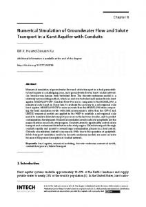
Particle concentrations Figure (6) shows the predicted and experimental (Holland-Batt and Holtham, 1991;Holtham,1992) values of

AFINIDAD LXXII, 571, Julio - Septiembre 2015

Fig.(7) The predicted values of mean-stream pulp velocity, at 15 % solids. water-velocity-magnitude

particle concentrations by volume in each stream. There is a good agreement between the predicted and the experimental values as shown in Figure. Particle concentrations by Volume (%)

60

Experimental

50

Predicted

2.28 2.072 1.864 1.656 1.448 1.24 1.032 0.824 0.616 0.408 0.2

STREAM FLOW- RATE The predicted values of stream flow-rate are shown in Fig. (9). It is clear from the figure that the stream flow-rate values depend on0.1the cross-sectional the mean 0.35 0.25 area 0.3 and 0.2 0.15 Radialstream. distance from central column (m) pulp-velocity of each Fig.(8) The predicted pulp-velocity contours (m/s), at 15 % solids.

30 20 10 0 1

2

3

4

5

6

7

30

Stream Flow Rate (% of Total)

40

8

Stream Number

25 20 15 10 5 0 1

Fig. (6) Predicted and experimental (Holland-Batt and Holtham, 1991; Holtham,1992) values of particle concentrations by volume in each stream, 15% solids in feed.

2

3

4 5 6 Stream Number

7

8

Fig. (9) Thevalues predicted values of stream Fig. (9) The predicted of stream flow-rate, at 15 % solids. flow-rate, at 15 % solids.

PULP VELOCITY STABILITY OF SOLID DISTRIBUTIONS

2,00 1,50 1,00 0,50 0,00

1

2

3

4

5

6

7

8

Stream Number Fig.(7) The predicted values mean-stream pulp Fig.(7) Theofpredicted values of velocity, mean- at 15 % solids. water-velocity-magnitude

2.28 2.072 1.864 2.28 1.656 2.0721.448 1.24 1.8641.032 1.6560.824 0.616 1.4480.408 1.24 0.2 water-velocity-magnitude

1.032 0.824 0.616 0.408 0.2 0.1

0.15

0.2

0.25

0.3

0.35

Radial distance from central column (m)

30

25 20

0.1

0.15

0.2

0.25

0.3

1,0E-09

First turn Sixth turn

1,0E-08 1,0E-07 1,0E-06 1,0E-05 1,0E-04 1,0E-03 1,0E-02 1,0E-01 1,0E+00

1,0E-09

Third turn Sixth turn

1,0E-08 1,0E-07 1,0E-06 1,0E-05 1,0E-04 1,0E-03 1,0E-02 1,0E-01 1,0E+00

0.35

1

Radial distance from central column (m)

1,0E-08

Second turn

1,0E-07

Sixth turn

1,0E-06 1,0E-05 1,0E-04 1,0E-03 1,0E-02 1,0E-01 1,0E+00

2

3

4

1

5

6

Stream Number

7

1,0E-09

2

3 4 5 6 7 Stream Number

8

Fourth turn Sixth turn

1,0E-08 1,0E-07 1,0E-06 1,0E-05 1,0E-04 1,0E-03 1,0E-02 1,0E-01 1,0E+00

1

8

2

3

4

5

6

Stream Number

7

8

Fig. (10) Change of the solid distributions with the number of turns 0.3% solidsof andthe 6 m3solid /hr flowdistriburate. Fig. (10) atChange

15 10

1,0E-09

1 2 3 4 5 6 7 8 Stream Number

Fig.(8) The predicted pulp-velocity contours (m/s), at 15 % solids.

tions with the number of turns at 0.3% solids and 6 m3/hr flow rate.

0 1

2

3

4 5 6 7 8 AFINIDAD LXXII, 571, Julio - Number Septiembre 2015 Stream

0,40 0,30

First turn Sixth turn

ction (Fraction)

5 ction (Fraction)

Stream Flow Rate (% of Total)

Fig.(8) The predicted pulp-velocity contours (m/s), at 15 % solids.

Mean Volume Fraction (Fraction)

Mean Volume Fraction (Fraction)

stream pulp velocity, at 15 % solids.

Mean Volume Fraction (Fraction)

Mean Velocity (m/s)

2,50

Solid distributions stability means the distributions at the steady-state condition or the final distributions at the end of the spiral trough. It is very17 important to investigate and predict the number of turns that is required for the stability of solid distributions. The number of enough spiral turns fulfills when the solid distributions become constant and do not change with increasing the number of turns. The constant solid distribution fulfills when agreement between predicted values of any spiral turn and stability distribution of spiral outlet is satisfied. In this study, the stability distribution is taken as the solid distribution at the end of the sixth turn of the spiral separator. This is because LD9 spiral separator has only six turns. The stability of solid distribution is predicted using two cases of solid percent, namely: 0.3% and 15%at flow rate of 6 m3/hr. For the above purpose, solid distributions on the spiral trough were chosen at the outlet of each spiral turn. The solid distributions of cases 0.3% and 15% solids are shown in Figs. (10) and (11), respectively.

Mean Volume Fraction (Fraction)

The predicted mean-stream pulp velocity for 15% solids is shown in Fig. (7).The mean-stream pulp velocity increases smoothly in the outward-direction away from the centerline of the spiral trough. The predicted pulp-velocity contours are shown in Fig.(8).

0,40 0,30

Second turn Sixth turn 227

1

2

3

4

5

6

7

Stream Number

1

8

2

3

4

5

6

Stream Number

7

8

Mean Volume Fraction (Fraction)

0,40

First turn Sixth turn

0,30 0,20 0,10 0,00

Mean Volume Fraction (Fraction)

1 2 3 4 5 6 7 8 Stream Number 0,40

0,20 0,10 0,00

2

3 4 5 6 7 Stream Number Mean Volume Fraction (Fraction)

1

Second turn Sixth turn

0,30 0,20

3.

0,10

8

2

0,40

3 4 5 6 7 Stram Number

8

Fourth turn Fifth turn

0,30

REFERENCES 1.

0,20

2. 0,10 0,00

1

2

3 4 5 6 7 Stream Number

8

0,40

3.

Fifth turn Sixth turn

0,30

4.

0,20

5.

0,10

6.

0,00

1

2

3 4 5 6 7 Stream Number

8

Fig. (11) Change of the solid distributions with the number of turns Fig. (11) Change of6 the distribuat 15% solids and m3/hrsolid flow rate.

7.

tions with the number of turns at 15% solids and 6 m3/hr flow rate.

8. Figures (10) and (11) show the solid distributions as a volume fraction. After the first spiral turn, the solid distriTables: butions are greater than the final distribution in the outer region of the spiral trough, while, it is lower in the inner Table (1) The geometrical parameters of LD9 spiral separator (Doheim et al.,2013) region. It means that the particulate-flow moves toward Inner Outer Trough Pitch Descent Number Curvature theRadius outer part of trough turn. After Radius Width at the u end of the first angle of Turnsthe ψ o ri(mm) spiral ro (mm) (mm)deviation (mm) α( ) distribution n second turn,Wthe between solid 70 350 280 273 decreases 0.75 7 - 32 6to the and final (stability) distribution comparing first turn. After the third spiral turn, the agreement between water depth and stability depth is about 95% in case of Table 2: The properties of usedthan particles 0.3% and less 95% in case of 15% solids. After the fourth turn, a complete agreement between the solid distributions and stability distributions is achieved in case of 0.3% solids while the complete 19 agreement in case of 15 % solids is satisfied after the fifth turn. This means that four turns of LD9 spiral separator are enough for the stability of the solid distributions in case of 0.3 % solids and five turns is required for stability in case of 15% solids. This point guides the designers to the suitable number of turns that is enough for the stability of solid distributions. This concept is very important for designers and operators.

9.

10.

11.

12.

13.

14.

CONCLUSIONS From this study, the following conclusions can be stated: 1. The suggested numerical model can be applied for any spiral separator after modifying the domain geometry to the required separator. 2. To improve the agreement between the predicted and the experimental results, the experimental free-surface profile was used to complete the computational

228

domain. This achieved a good agreement between the model predictions and the experimental results. Thus, validation of the particulate-flow model is satisfied. The number of turns required to reach the steadystate of particle size distribution increases with increasing the solid content of the feed pulp.

0,00

1

Third turn Sixth turn 18

0,30

0,40

Mean Volume Fraction (Fraction)

Mean Volume Fraction (Fraction)

Fig. (10) Change of the solid distributions with the number of turns at 0.3% solids and 6 m3/hr flow rate.

15.

16.

Burch CR (1962). Helicoid Performance and Fine Cassiterite-Contributed Remarks. Trans. Inst. Min. Metall.71:406-415. Doheim MA, Abdel Gawad AF, Mahran GMA, Abu-Ali MH , Rizk AM(2013). Numerical Simulation of Particulate-Flow in Spiral Separators: Part I, low solids Concentration (0.3 & 3% solids). Applied Mathematical modeling 37(1):198-215. Escue A, Cui J(2010). Comparison of turbulence models in simulating swirling pipe flows. Applied Mathematical Modelling 34(10) :2840–2849. Ferziger,J. H. and Peric, M.,(1999). Computational methods for fluid dynamics. Second edition, Springer. Fluent 6.3.26 User’s Guide (2006), www.fluentusers. com, Fluent Inc., USA. Holland-Batt AB, Holtham PN (1991). Particle and Fluid Motion on Spiral Separators. J.Minerals Engineering 4(3-4): 457-482. Holland-Batt, A. B. (1995) .Some design considerations for spiral separators. Minerals Engineering, Vol. 8, No. 11 pp.1381-1395. Holtham PN (1992). Particle transport in gravity concentrators and the Bagnold effect.Minerals Engineering 5(2): 205-221. Holtham PN (1997). Experimental validation of a fundamental model of coalspirals. Australian Coal Association research program (ACARP). Jancar T, Fletcher CAJ, Holtham PN, Reizes JA (1995). Computational and Experimental Investigation of Spiral Separator Hydrodynamics. Proc. XIX Int. Mineral Processing Congress, San Francisco, USA. Jancar ML, Holtham PN, Davis JJ, Fletcher CAJ. (1995). Approaches to the development of coal spiral models. An International symposium, Soc. Mining, Metal and Exploration, Littliton, USA, pp. 335-345. Kuang S, , Qia Z, Yua AB, Vinceb A, Barnettc GD, Barnettc PJ(2014). CFD modeling and analysis of the multiphase flow and performance of dense medium cyclones. Minerals Engineering 62:43–54. Loveday GK, Cilliers JJ (1994). Fluid flow modelling on spiral concentrators. Minerals Engineering, Vol. 7, Nos. 2-3, pp. 223-237. Machunter DM., RichardsRG, Palmer M K (2003). Improved gravity separation systems utilizing spiral separators incorporating new design parameters and features”, Heavy Minerals Conference (HMC) 2003,Johannesburg, South African Institute of Mining and Metallurgy,2003 Matthews BW, Fletcher CAJ, Partridge AC (1998b). Computational Simulation of Fluid and Dilute Particulate Flows on Spiral Concentrators. Applied Mathematical Modelling 22 :965-979. Matthews BW, Fletcher CAJ, Partridge AC, Vasquez S (1999a). Computations of Curved Free Surface Water

AFINIDAD LXXII, 571, Julio - Septiembre 2015

17.

18.

19.

20.

21.

22.

23.

Flow on Spiral Concentrators. J. Hydraulic Engineering 125 (11):1126-1139. Mathews BW, Fletcher CAJ, Partridge TC (1999b). Particle Flow Modeling on spiral concentrators: Benefits of dense media for coal processing?. Second International Conference on CFD in the Minerals and Process Industries, CSIRO, Melbourne, Australia, 6-8 December, 1999. Matthews BW, Holtham P, Fletcher CAJ, Golab K, Partridge AC,( 1998a). Computational and Experimental Investigation of Spiral Concentrator Flows. Coal 1998: Coal Operators’ Conference, University of Wollongong & the Australasian Institute of Mining and Metallurgy, 415-421. Mishra BK, Tripathy A (2010). A preliminary study of particle separation in spiral concentrators using DEM. International Journal of Mineral Processing 94( 3-4):192–195. Radman JR, Langlois R, Leadbeater T , Finch J, Rowson N, Kristian Waters K (2014). Particle flow visualization in quartz slurry inside a hydrocyclone using the positron emission particle tracking technique. Minerals Engineering 62: 142–145 Stokes YM, Wilson SK, Duffy BR (2004). Thin-Film Flow in Open Helically-Wound Channels. 15th Australasian Fluid Mechanics Conference, 13-17 December 2004,The University of Sydney, Sydney, Australia. Wang JW, Andrews JRG (1994). Numerical Simulations of Liquid Flow on Spiral Concentrators. J. Minerals Engineering 7(11):1363-1385. Yakhot V, Orszag SA (1986). Renormalization Group Analysis of Turbulence I. Basic Theory. Journal of Scientific Computing 1 (1): 1-51.

AFINIDAD LXXII, 571, Julio - Septiembre 2015

229