PD-based Model Predictive Control of ... - IEEE Xplore

This article has been accepted for publication in a future issue of this journal, but has not been fully edited. Content may change prior to final publication. Citation information: DOI 10.1109/TBME.2015.2497273, IEEE Transactions on Biomedical Engineering

TBME-00023-2015

1

Robust PBPK/PD-based Model Predictive Control of Blood Glucose Stephan Schaller, Jörg Lippert, Lukas Schaupp, Thomas R. Pieber, Andreas Schuppert, and Thomas Eissing Abstract— Goal: Automated glucose control (AGC) has not yet reached the point where it can be applied clinically [3]. Challenges are: accuracy of subcutaneous (s.c.) glucose sensors, physiological lag-times, and both inter- and intra-individual variability. To address above issues, we developed a novel scheme for MPC that can be applied to AGC. Results: An individualizable generic whole-body physiologybased pharmacokinetic and dynamics (PBPK/PD) model of the glucose, insulin, and glucagon metabolism has been used as the predictive kernel. The high level of mechanistic detail represented by the model takes full advantage of the potential of MPC and may make long-term prediction possible as it captures at least some relevant sources of variability [4]. Robustness against uncertainties was increased by a control cascade relying on proportional, integrative, derivative (PID)-based offset control. The performance of this AGC scheme was evaluated in silico and retrospectively using data from clinical trials. This analysis revealed that our approach handles sensor noise with a MARD of 10-14%, and model uncertainties and disturbances. Conclusion: The results suggest that PBPK/PD models are well suited for MPC in a glucose control setting, and that their predictive power in combination with the integrated databasedriven (a-priori individualizable) model framework will help overcome current challenges in the development of AGC systems. Significance: This work provides a new, generic and robust mechanistic approach to AGC using a PBPK platform with extensive a-priori (database) knowledge for individualization. Index Terms—artificial pancreas, decision support, diabetes, glucose metabolism, patient variability, physiology-based pharmacokinetics and pharamcodynamics predictive control, predictive models.

(PBPK/PD),

Submitted for review on 20.05.2014. S.S., J.L., T.E., L.S. and T.R.P. acknowledge partial financial support by the European Commission, under Grant Agreement 248590 (FP7 Integrated Project Reaction; Remote Accessibility to Diabetes Management and Therapy in Operational Healthcare Networks). S.S., A.S., and T.E. are with Computational Systems Biology, Bayer Technology Services GmbH, 51368 Leverkusen, Germany, ([email protected], [email protected], [email protected]). S.S. and A.S are also affiliated with the Aachen Institute for Advanced Study in Computational Engineering Sciences, RWTH Aachen, Aachen, Germany, 52062 Aachen, Germany ([email protected]). J.L. has been with Computational Systems Biology, Bayer Technology Services GmbH, and is now with Clinical Pharmacometrics, Bayer Pharma AG, 42113 Wuppertal, Germany ([email protected]). L.S. and T.R.P. are with the Department of Internal Medicine, Medical University of Graz, 8036 Graz, Austria ([email protected], [email protected]).

I. INTRODUCTION

D

IABETES mellitus is a chronic disease that affects a continuously growing population of currently over 380 million patients worldwide [5]. Type 2 diabetes (T2DM) accounts for 85% to 95% of all diabetes. It is caused by a defect in the body’s autonomous regulation of blood glucose, which is normally managed by complex interactions among neuronal, hormonal, and metabolic-signaling networks. Type 1 diabetes (T1DM), although less common, has a high prevalence in children and adolescents and is caused by an autoimmune reaction damaging the insulin producing beta cells of the pancreas. Currently, T1DM and severe cases of T2DM can only be controlled by the affected individual, through constant vigilance and manual insulin therapy. Effective automated control of blood glucose levels could theoretically reduce the burden of manual therapy and improve the risk profiles of most patients with type 1 diabetes mellitus (T1DM). Additional benefits would include improved quality of life and reduced costs [6]. An integrated system that combines a subcutaneously implanted continuous glucose monitor (CGM) and an insulin infusion pump (IIP) is often referred to as an “artificial pancreas” (AP). Although AP systems have been under development for over 50 years, they are still not capable of orchestrating everyday control of blood glucose. This is due to both technical and system-inherent hurdles, including: (a) insufficient accuracy of CGM devices, (b) the lag times of subcutaneous (s.c.) glucose measurements when changes in blood glucose levels are rapid, (c) the lag time for the onset of insulin action after s.c. insulin administration, and (d) the lingering/tailing action of insulin action after s.c. administration [3, 7, 8]. Recent improvements in the accuracy of s.c. CGM devices, IIPs and safety systems have enhanced conditions for developing a fully integrated AP system [8, 9]. Also, the superiority of AGC involving both s.c. measurement of glucose and s.c. infusion of insulin (the s.c.-s.c. route) over manual control of glucose levels has been demonstrated in clinical trials [10]. Various strategies for controlling blood glucose, ranging from proportional, integrated, derivative (PID) [11-17] to complex fuzzy logic methods [18, 19], have been used in designs for the AP. Nevertheless, physiologic lag times remain a core problem in reactive (i.e. PID) feedback-control solutions [20]. These lag-times are better addressed using

0018-9294 (c) 2015 IEEE. Translations and content mining are permitted for academic research only. Personal use is also permitted, but republication/redistribution requires IEEE permission. See http://www.ieee.org/publications_standards/publications/rights/index.html for more information.

This article has been accepted for publication in a future issue of this journal, but has not been fully edited. Content may change prior to final publication. Citation information: DOI 10.1109/TBME.2015.2497273, IEEE Transactions on Biomedical Engineering

TBME-00023-2015 predictive control solutions, and model predictive control (MPC) is the most widely used among these [21-27]. Key components of such MPC approaches are mathematical models of the biological processes relevant to glucose control. Early models only vaguely reflected the physiological structures involved, in spite of the fact that these are vital to comprehending the influence of lag-times. Research to improve these models focused on more physiology-based model concepts, as model-based glucose control requires reliable models with longer-term predictive capabilities. Recently, the UVa/Padova simulator, which is based on a model by Dalla Man et al. [28], proved sufficiently effective to receive approval from the U.S. Federal Drug Administration (FDA) as a replacement for animal testing of glucose controllers [29]. In addition, the Cambridge Model developed by Hovorka et al. [30] for closed-loop glucose control incorporates physiological aspects and represents the current state of the art in glucose modeling as it applies to model-based glucose control. However, even these more physiological models fail to scale key parameters such as blood flow, organ volume, and subcompartment size to an individual’s anthropologic properties. A fully physiological modeling framework such as that described in [4] allows for a priori individualization of these properties of the model with respect to age, weight, height, gender, and race. We have developed a control approach that combines, for the first time, a detailed a priori individualizable generic whole-body, physiology-based pharmacokinetic and dynamics (PBPK/PD) model of the glucose-insulin metabolism (GIM) [4] with a robust MPC algorithm for AGC in a post-hoc in silico study. Based on this accurate model for predicting the core dynamics of blood glucose levels (i.e. in the undisturbed state) in an individual, and adapting over time by adding continuously gathered patient data, the MPC computes an optimal feed-forward control input. To increase closed-loop stability as well as robustness against both disturbances and model uncertainties, we use a PID-based feedback controller that compensates for prediction errors (offset). Here we test, in silico, the performance of the control algorithm in a simulated control trial, in the face of measurement error, model uncertainty and disturbances. II. MATERIALS & METHODS The glucose control framework developed here allows both in silico evaluation of controller concepts and control of blood glucose in T1DM patients in a clinical setting. The interactions among the components of the integrated system are based on the modular approach described in [8]. The three interacting layers work on different timescales (Appendix Fig. 5). The outer layer is on a slow timescale and adjusts the parameters of the inner, fast layer. In the system described here, the outer layer is represented by model adaptation, i.e. “offline optimization,” using glucose measurement data to adjust the model kernel of the MPC (middle layer). The MPC, i.e. “online simulation & control,” in turn, calculates insulin delivery based on the prediction of blood glucose levels and meal information. The middle layer is further restricted by the

2

inner layer, i.e. the robustness layer, which is comprised of the offset-controller (PID). It constantly adjusts 1) the blood glucose target value for the MPC and 2) the insulin doses calculated by the MPC. The insulin adjustments are based on the latest CGM data (and the predictive error), incorporating algorithms for pump shutoff and insulin-on-board constraints. Once the integrated system is in place, various increasingly complex configurations of an AP system become possible. A. Individualized Physiology-Based Models and Software PBPK models describe the mechanisms underlying the absorption, distribution, metabolism, and excretion (ADME) of a substance within the body in great detail. Such models are based to a large extent on prior information. This information is taken from collections of anatomical and physiological data, and calculations are made based on the drug’s physiochemical properties and their effects on various organs and tissues, taking into account an organism’s anatomy and physiology and its changes with age, as well as its weight, height, gender, and race (e.g. age dependence of organ weights, blood flows). Also, the information about how active processes (e.g. metabolic rates, transport and clearance rates) scale with relation to these properties is integrated. Generic, adult PK prediction models can automatically be parameterized based on the basic physicochemical parameters of a substance, and can then be used to simulate drug-concentration profiles in various organs and tissues [31]. Once an adult PBPK model has been established, it can be extrapolated to individuals—be it adults, children or elderly—outside of the selected cohort [32]. The PBPK models for glucose, insulin and glucagon [4] were established in the PK-Sim® 5.1, and coupled in the MoBi® 3.1, commercial software packages for PBPK modeling and molecular biology modeling, respectively [1, 31]. Model identification, model parameterization, and the development of control algorithms were conducted using the MoBi® Toolbox for MATLAB® 3 and MATLAB® 2012 (The MathWorks, Natick). B. Generating Virtual Patients The model used to generate the in silico subjects in the simulation environment was previously described in detail and validated, including how the parameters for the generic model were set [4]. This model was fitted to a dataset collected for 12 T1DM patients studied in a 2-phase randomized crossover trial (2PRCT, from the project Advanced Insulin Infusion using a Control Loop (ADICOL) [33], and the effectiveness of continuous s.c. insulin infusion (CSII) was compared to that of an MPC system (Cambridge Algorithm (CA) [33])), generating 12 virtual patients. In the absence of s.c. glucagon infusion and mean meal-independent parameters for oral glucose absorption, the algorithm identifies 6 parameters (first 6 in Table II, Appendix) for model individualization (also in [4], supporting information Table S3) from the blood glucose measurement data, and then fits the generic model to the respective patient data to generate a virtual patient. Thus, the in silico subjects used for the in silico validation and the MPC algorithm presented here use the exact same

0018-9294 (c) 2015 IEEE. Translations and content mining are permitted for academic research only. Personal use is also permitted, but republication/redistribution requires IEEE permission. See http://www.ieee.org/publications_standards/publications/rights/index.html for more information.

This article has been accepted for publication in a future issue of this journal, but has not been fully edited. Content may change prior to final publication. Citation information: DOI 10.1109/TBME.2015.2497273, IEEE Transactions on Biomedical Engineering

TBME-00023-2015 model as presented in [4]. The models may only differ by their physiologic values (e.g. physiology dependent (calculated) properties like blood volume) and the 6 identified parameters used for model individualizations (the MPC is initialized with mean population values for these 6 parameters). To parameterize the model, the fmincon function of the MATLAB® optimization toolbox was used with a quadratic penalty function. C. Design of In Silico Clinical Trial The in silico trials evaluating the integrated algorithms were carried out using the protocol described above for the 2PRCT. The control inputs used were constant insulin infusions over 15 min, corresponding to the sampling time for blood glucose values and CGM readouts (note that although CGM readouts were taken every 5 min, due to the need for manual handling every 3rd readout was deemed sufficient). In the 2PRCT protocol, the subjects were admitted to the clinical research center at the Medical University of Graz (MUG) at 2 p.m.. Prior to the first meal on the day of arrival, from 2 p.m. until 5 p.m. (t = 0-180 min), the study started with a glucose clamp and subjects were adjusted to 100 mg/dl blood glucose and received basal insulin via a pump until closed-loop control was initiated following the first meal. Over the course of the trial, the subjects (N = 12) received 4 meals. Dinner (the first meal) was provided at 6 p.m. (t = 240 min), and closed-loop glucose control was initiated at 7:30 p.m. (t= 330 min, end of observation phase) and continued until 10 p.m. the following day. On the second day, the subjects received meals at 7 a.m. (t = 1020 min, breakfast), 12 p.m. (t = 1320 min, lunch), and 6 p.m. (t = 1680 min, dinner). Meal information was transferred to the controller at the time of meal onset, such that prandial insulin was not infused prior to the meals. The target range for insulin was defined as 70–180 mg/dl 3h postprandial and 70–140 mg/dl at all other times. “OVERALL” refers to the duration of the trial (7:30 p.m., Day 1 to 10 p.m., Day 2), “DAYTIME” to the time from the end of breakfast to the end of trial (8 a.m., Day 2 to 10 p.m., Day 2), and “OVERNIGHT” to the nighttime period during the trial (10 p.m., Day 1 to 8 a.m., Day 2). Throughout the trial, the control input was calculated every 15 min, when the blood glucose was sampled. D. Control Algorithm The effectiveness of model-based glucose control algorithms depends on the model kernel being tuned to the system it controls. In the case of blood-glucose control, the model is tuned for each patient using experimental data gathered over time [12]. The study described here tests our robust MPC algorithm in an in silico trial, using the protocol described above. During this trial, glucose measurements from simulated virtual patients were used to individualize the kernel on which the MPC operates. The algorithm first establishes a mean model of GIM, and this is then scaled based on the physiologic properties (age,

3

weight, height, gender and race) of the enrolled patient. Model individualization is started with the first blood-glucose measurement at 2 p.m. on Day 1. As the efficient use of time for model individualization (finding a timely solution to the optimization problem) is paramount, a virtual population was generated a priori based on the known physiologic properties (e.g. age, weight and height) of the patient, but with variations the individual parameter set (first 6 parameters in Table II, Appendix) taken from distributions pre-calculated based on known model parameterizations [4]. The resulting virtual population was then screened for the best fit to data collected during the clamp phase (observation phase), i.e. from 2 p.m. until 7:30 p.m. on the first day. The best-fit parameter set was used to initiate the MPC at 7:30 p.m., with the optimal insulin dose, 𝑢𝑀𝑃𝐶 (𝑡), calculated based on predictions of the model (Appendix Fig. 5). The AGC continuously improves the model kernel used by the MPC over the course of the trial, as more data becomes available. The individual parameter set is constantly optimized based on all measurement data collected up to that point. A “Growing Horizon Estimatior” (Appendix Fig. 7) is used to this end. However, this feature was deactivated for the purposes of the in silico analysis described here. The evaluation of controller performance in the context of suboptimal fit of the model, i.e. in the presence of model uncertainty, required that the model was not adapted following the initial matching. This initially matched model is suboptimal in the sense that the match from the initial population is based on a coarse grid search over the range of the parameters, and does not necessarily reflect the optimal parameters for the individual. The algorithm, which was run on a standard laptop PC, was implemented in MATLAB® and controlled via a graphical user interface (GUI using MATLAB® GUIDE). For model adaptation and input optimization, we use the functions fmincon and fminbnd, respectively, of the MATLAB® optimization toolbox. The parameters used to configure the controller are provided in Table III (Appendix). 1) Model Predictive Control MPC is a form of control in which the “current” control action is determined by solving, at each sampling instant, a finite-horizon open-loop optimal control problem, 𝑃(𝒙, 𝒌). A schematic of the general concept is shown in Appendix Fig. 7. Optimization of the cost function 𝑉(𝒙, 𝒌, 𝒖) at time 𝑘 = 𝑡𝑘 , subject to any imposed control, state and terminal constraints, yields an optimal control sequence 𝒖 of 𝑁 piecewise constant control inputs, and the first control in this sequence at time 𝑘 = 𝑡𝑘 is applied to the controlled system [2, 34]. This produces a closed-loop control strategy, solving an open-loop optimization problem. The general control problem is defined as: 𝑃(𝒙, 𝒌) = min 𝑉(𝒙, 𝒌, 𝒖) (1) 𝒖 with the discretized point in time 𝑡𝑘 , and the general cost function:

0018-9294 (c) 2015 IEEE. Translations and content mining are permitted for academic research only. Personal use is also permitted, but republication/redistribution requires IEEE permission. See http://www.ieee.org/publications_standards/publications/rights/index.html for more information.

This article has been accepted for publication in a future issue of this journal, but has not been fully edited. Content may change prior to final publication. Citation information: DOI 10.1109/TBME.2015.2497273, IEEE Transactions on Biomedical Engineering

TBME-00023-2015 𝑘+𝑁

𝑉(𝒙, 𝒌, 𝒖) = ∑ 𝑙(𝑥𝑖 , 𝑢𝑖 ) + 𝐹(𝑥𝑘+𝑁 )

(2)

𝑖=𝑘

with stage cost 𝑙, the optimized input sequence 𝒖 = {𝑢𝑘 , 𝑢𝑘+1 , … , 𝑢𝑘+𝑁−1 }, system state 𝑥𝑖 (corresponds to either plasma (i.v.) glucose or s.c. glucose), and terminal cost 𝐹(𝑥𝑘+𝑁 ). However, this is a multidimensional optimal control problem that uses a sequence of piecewise constant inputs 𝒖 = {𝑢𝑘 , 𝑢𝑘+1 , … , 𝑢𝑘+𝑁−1 }, and thus solving it may become computationally demanding. A common approach to saving computational time and increasing the speed of convergence of the optimization problem is to restrict optimization to the first input of the sequence. The cost function is then defined as:

4

of model inaccuracy (i.e. a model drift), most of the insulin input will be calculated by the MPC rather than by the feedback controller. This is to ensure timely control action, as the MPC is a (feed-forward) predictive controller, and shifting influence to the reactive FMPD feedback component (i.e. the input correction ∆𝑢(𝑡)) as the determinant of input would lead to a reduction in overall response time. ∆𝑇𝑉 is calculated from the relative prediction error 𝑒(𝑡) = 𝑥(𝑡) − 𝑦(𝑡), such that 𝐷𝑦𝑛𝑎𝑚𝑖𝑐 𝑇𝑉 = 𝑇𝑉 + ∆𝑇𝑉 and ∆𝑇𝑉(𝑡 = 0) = 0. In the context of fading memory, this gives: 𝑡

∆𝑇𝑉 = 𝐾𝑝 ∫ e

𝑡 −𝑊𝑝 (𝑡−𝜏)

0

𝑘

𝑗=0

(3)

𝑖=𝑘

yielding the feedback control law: 𝑢0 = 𝑢𝑘0 .

0

𝑘

(4)

2) Offset-Control/Error Compensation (PID) To increase the robustness of the chosen MPC AGC approach, we use a PID-based offset controller here. The development of such a controller is based on basic concepts of feedback control [35, 36]. In general, a PID controller is based on three characteristics of the output tracking error 𝑒(𝑡) in relation to a (constant) target value: the weighted current absolute error (proportional component, P); the weighted sum of all past errors (integral component, I); and the weighted change in error compared to the error at the last sampling point (derivative component, D). These three components are summed in calculating the control input (Appendix Fig. 5). The offset controller is introduced for two reasons: to compensate for inaccuracies of the model fit and to reject disturbances. Even a detailed PBPK/PD model does not fully account for all dynamics that may cause an observed change in blood glucose levels. The offset controller filters the residual error of the model predictions made by the MPC (Appendix Fig. 5). Thus, the tracking error 𝑒(𝑡) corresponds to a prediction error and is calculated as deviation of the simulated blood glucose prediction, 𝑥(𝑡), from the actual blood glucose measurements, 𝑦(𝑡) (for more details on simulated concentrations see Appendix A). Based on these values, the offset-controller calculates two corrections via a feedback loop based on the prediction error, 𝑒(𝑡). The first is the set-point correction ∆𝑇𝑉 (i.e. a shift in target value) of the MPC. The second is the control input correction, ∆𝑢(𝑡), which corrects the insulin infusion recommendations 𝑢𝑀𝑃𝐶 (𝑡) made by the MPC. To increase the robustness of offset control against sensor noise and disturbances, the fading memory principle from Fading Memory Proportional Derivative control (FMPD) [1215] was adapted for the P and D components. The reason a dynamic target value correction, ∆𝑇𝑉, is used is that in spite

(5)

≈ 𝐾𝑝 ∑ e−𝑊𝑝 (𝑘−𝑗) 𝑒𝑗 + 𝐾𝑖 ∑ 𝑒𝑗 .

𝑘+𝑁

𝑉(𝒙, 𝒌, 𝒖) = ∑ 𝑙(𝑥𝑖 ) + 𝑢𝑘

𝑒(𝜏)𝑑𝜏 + 𝐾𝑖 ∫ 𝑒(𝜏)𝑑𝜏

𝑗=0

with the controller gains 𝐾 and the forgetting factor 𝑊𝑝 , in the case of the proportional component, where 𝑊𝑝 determines how rapidly past values fade from memory. We chose to use an exponentially decaying fading function. The derivative component was not included in calculating ∆𝑇𝑉, as this would increase the influence of sensor noise. The integral component was included to accommodate for the effects of model nonlinearity, ensuring that the set-point (dynamic target value) error would be zero. A drawback of dynamic shifting of the target value is that it could lead to nonlinear behavior of some components of the GIM model. This could “distort” the estimate of the insulin dose required, due to nonlinearities inherent to the model. However, individualization of the model kernel ultimately reduces the required shift, diminishing the influences of nonlinearities. The reason for using only the proportional and integral components in calculating ∆𝑇𝑉 is that this value should compensate solely for the overall drift in predictive error; short-term deviations and disturbances are corrected by the input correction, in particular by its derivative component. The second component, ∆𝑢(𝑡), of the offset controller corrects the input MPC dose calculations, 𝑢𝑀𝑃𝐶 (𝑡). The calculation of this error also takes into account the shift in target value for the MPC controller, correcting only any remaining deviations. This prediction error of 𝑒̂ (𝑡) = ∆𝑇𝑉 − 𝑒(𝑡) takes into consideration the dynamic shift ∆𝑇𝑉 of the MPC such that the input correction ∆𝑢(𝑡) approaches zero once the target value is shifted by the value of the prediction error (𝑒(𝑡) = ∆𝑇𝑉). A generalized formulation of the FMPD control for the calculation of the input correction ∆𝑢(𝑡) is: 𝑘

∆𝑢𝑘 = 𝐾𝑝 ∑ e

𝑘 −𝑊𝑝 (𝑘−𝑗)

𝑒̂𝑗 + 𝐾𝑖 ∑ 𝑒̂𝑗

𝑗=0

𝑗=0

(6)

𝑘 −𝑊𝑑 (𝑘−𝑗)

+ 𝐾𝑑 ∑ e

(𝑒̂𝑗 − 𝑒̂𝑗−1 ).

𝑗=0

The input correction was tuned to respond more rapidly to changes in 𝑒(𝑡). The tuning of the forgetting factors 𝑊𝑝 and 𝑊𝑑 within a real control setting is always a trade-off between susceptibility to sensor error/noise and an increase in time

0018-9294 (c) 2015 IEEE. Translations and content mining are permitted for academic research only. Personal use is also permitted, but republication/redistribution requires IEEE permission. See http://www.ieee.org/publications_standards/publications/rights/index.html for more information.

This article has been accepted for publication in a future issue of this journal, but has not been fully edited. Content may change prior to final publication. Citation information: DOI 10.1109/TBME.2015.2497273, IEEE Transactions on Biomedical Engineering

TBME-00023-2015 delay or “sluggishness” of the controller. As the derivative component represents the rapid first-response characteristic of a beta cell, a larger factor (and thus faster memory decay) was chosen. Both MPC (penalty function) and offset-control are subject to additional safety constraints and parameterizations, as documented in the Appendix. Although our results indicate that the MPC control algorithm is robust even in the context of significant prediction error, a key feature is that when the model kernel is used in a clinical-trial setting it will be continuously updated as new measurements become available. A standard optimization routine (fmincon, MATLAB®) was chosen for optimizing the individual parameter set [4] in this context. E. Method for In Silico Controller Evaluation We have tested our control system against 12 in silico individuals, with the model parameterized based on the 2PRCT data. We evaluated the robustness of the controller in the setting of three potential sources of variability: 1) model uncertainties, using a suboptimal fit of the internal MPC model kernel; 2) disturbances, e.g., the unanticipated intake of carbohydrates; and 3) sensor error, e.g., simulating sensor noise of both intravenous (i.v.) und s.c. glucose measurements. For the MPC algorithm a prediction horizon of 𝑁 = 240 min (6 h) was chosen. The dose of insulin, which was infused at constant rate over a 15 min period, was calculated by solving the nonlinear constrained optimization problem described in (1). The in silico trials for evaluating the integrated algorithms were carried out using the same protocol as in the 2PRCT. As mentioned in Section 2D, we did not adapt the model following the initial matching with the starting population. Given that this study was carried out in preparation for in vivo clinical trials, we evaluated two scenarios—one in which i.v. measurement of glucose was simulated, and another in which CGM (s.c.) measurement of glucose was simulated. The first scenario is for controller evaluation using simulated i.v. measurements of glucose with a mean standard deviation of 5%. This case was used to simulate the Super GL 2 instrument (Dr. Müller Gerätebau GmbH, Freital, Germany; expected measurement error for such measurements is 500 min), the offset controller did not reduce the insulin dose. This reactive control behaviour slightly restricts the predictive capabilities of the MPC and causes the glucose trajectories to oscillate. Especially in the context of high insulin doses (e.g. prandial insulin), an underestimate of the half-life of insulin action (i.e.

6

meal, occurs and triggers a rise in glucose that is substantially faster than insulin can be absorbed and exert its activity [8]. Another type of disturbance that can trigger such problems is a change in metabolism, e.g. as a consequence of exercise, stress or medical treatment. For the purpose of evaluating the model’s ability to reject disturbances, an intake of 1 glass of orange juice (12 g

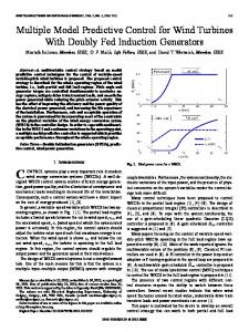
Fig. 3. In silico evaluation of controller across the virtual cohort by control variability grid analysis (CVGA, 100%tile). The CVGA displays the minimal (x-axis) to maximal (y-axis) glucose values (range of control) for all (simulated) measurements for each individual. Left: Variability in control for duration of the trial (7:30 p.m., Day 1 to 10 p.m., Day 2). Right: Variability in control overnight (10 p.m., Day 1 to 8 a.m., Day 2). More details on control performance are given in Table I and II and Fig. 4.

glucose) was triggered at 4 p.m. on day 2 (t = 1560 min). As shown for Subject 06 in Fig. 2, the resulting discrepancies between the model predictions and measurements trigger both a rapid reaction by the offset-controller and a slow and steady shift from the dynamic target value. In spite of an overprediction of the half-life of insulin, the disturbance is managed well and does not result in a controller overreaction.

Fig. 2. Effects of disturbances on glucose concentration, insulin infusion, and insulin concentration. Representative in silico run, carried out for Subject 06. Symbols and conditions of experiment are as described for Fig. 1.

overestimation of insulin clearance) can have serious consequences; in this example the large insulin dose at breakfast at time t = 1100 min resulted in postprandial low glucose levels at t = 1250 min as the decline of insulin action/levels was slower than that predicted by the MPC. However, overall the glucose trajectories stayed well within the target range, even after a glucose disturbance occurred at t = 1560 min (as elaborated in next section). 2) Effects of Disturbances Even with improvements in the sensor and pump technologies, AGC continues to rely on the controller being able to cope with both inaccuracies in glucose sensing and delays in insulin action. These issues are particularly problematic when a system disturbance, e.g. an unannounced

3) Effects of Error/Noise and Overall Performance The control algorithm for glucose measurements was tested on measurements with a MARE of 5%. Although the algorithm will first be evaluated in a clinical setting in which measurement will be i.v., dosing will be s.c. and the expected MARE will be below 2% (a higher simulated MARE was chosen for the purpose of making the evaluation conservative). As our results show (Figs. 1,2), noise at the level chosen for the simulation did not have a significant adverse effect on glucose control. To assess overall performance of the control system throughout the cohort, we performed control variability grid analysis on the control results (CVGA, Fig. 3) [39]. This revealed that the glucose trajectories were well within the normoglycemic range; episodes of hypoglycemia were absent. Also, the nighttime control (Fig. 3, right panel) was completely within the target range, with the mean blood glucose level only slightly above target value. More details on control performance are given in Table I and II and Fig. 4. B. In silico Evaluation of Online Controller (s.c. Measurement of Glucose) As a step forward and for the sake of compatibility with current state-of-the-art systems, the algorithm for glucose control in subjects with T1DM was adapted to work with s.c. measurements of glucose from CGM devices (e.g. Dexcom G4 Platinum, MARE of 10.8 ± 9.9% [38], with glucose

0018-9294 (c) 2015 IEEE. Translations and content mining are permitted for academic research only. Personal use is also permitted, but republication/redistribution requires IEEE permission. See http://www.ieee.org/publications_standards/publications/rights/index.html for more information.

This article has been accepted for publication in a future issue of this journal, but has not been fully edited. Content may change prior to final publication. Citation information: DOI 10.1109/TBME.2015.2497273, IEEE Transactions on Biomedical Engineering

TBME-00023-2015 readouts every 5 min). This integrated system has been

Fig. 4: Summary of sensor error-dependent performance of control. Each large circle represents a trial using a virtual cohort (n=12) to evaluate the effects of error (expressed as MARD in %) and the delay (up to 30 min) in s.c. measurements. The left part (x-axis points 3-17) represents in silico trials with artificially generated continuous glucose-monitor (CGM) sensor noise, and the right part (x-axis point 5) represents the in silico trial with simulated i.v. measurements (no delay). Each chart shows (as % of total time) the time at target concentration, the time above 140 mg/dl (hyperglycemia), the time below 70 mg/dl (mild hypoglycaemia) and the time below 50 mg/dl (hypoglycaemia). The colours indicate whether control performance is good (green), sub-optimal (orange) or critical (red). Specifically, for each sector, the colours reflect the following: time at target concentration: green >80%, orange 60%–80%, red 0% but 1 %. All values marked as orange are acceptable under controlled conditions.

thoroughly evaluated in silico in an extensive robustness analysis that assesses measurement errors and potential time delays associated with s.c. methods of measurement. The ultimate aim is to define accuracy criteria for the required sensor system. For each of the 12 in silico patients, we tested 15 artificial error/time-delay sets, producing a total of 180 trial runs. The error/time-delay sets were assembled based on the assumption that sensor error would range from 3–17% MARE, and that the delay would range from 0–30 min. The results of the robustness analysis are depicted in a traffic-light plot (Fig. 4). They indicate that an increase in MARE leads to an overall reduction in glucose levels as the % of time at target increases (for the zero time-delay cases), but also to an increase in the prevalence of hypoglycaemic events. In contrast, increasing the time delay increases the prevalence of hyperglycaemia due to increased glucose fluctuations. IV. DISCUSSION We have developed a novel approach to individualized AGC by integrating, for the first time, a detailed generic whole-body PBPK/PD model [4] into a robust MPC algorithm. We evaluated the effectiveness of this approach in controlling glucose by carrying out a post-hoc in silico study. The algorithm was tested against model uncertainty using suboptimal model fits, with the scenarios tested incorporating glucose-sensor noise and unprogrammed carbohydrate disturbances. As input, the algorithm requires only the individual’s physiologic properties (height, weight, gender and age) and the quantities of carbohydrates consumed. We found that the combination of a predictive system (MPC) with a reactive system (FMPD) significantly increases the

7

controller’s robustness with respect to uncertainty. All control insulin inputs are calculated and no additional pre-meal insulin bolus is required. Overall, the controller performs well. Although most systems currently available have been developed for s.c. measurement of glucose, the controller developed here uses a novel PBPK/PD model kernel and, because its initial clinical testing will be done using measurements of plasma glucose (for safety reasons), our in silico evaluation included this procedure. Many algorithms have been developed for AGC [40-42]. Among these, MPC is currently favored for a number of reasons: it is a predictive approach that can manage time delays inherent to the system (s.c. glucose monitoring and s.c. insulin infusion); it is model-based, which allows for straightforward personalization using patient-specific parameterization [43]; and it is optimization-based, making it possible to integrate performance specifications by constraining states (i.e. penalizing for hypoglycaemia) and inputs (insulin or glucagon infusion). The common approach of AGC using MPC is to adapt, in addition to global model adaptation (time-invariant patientspecific parameterization), a single input-output sensitive parameter per sampling time. This accounts for process variability over time (intra-individual or intra-day variability), and results in a discrete time-dependent profile for this parameter. Usually a parameter representing insulin sensitivity in the model is chosen for this time-dependent adaptation [22, 44]. Feed-forward calculation of the control input is then also based on sensitivity identified using past measurement data. In this study, only a global time-invariant patient-specific adaptation of the model was conducted (model individualization using all available measurement data) to improve prediction of the individual’s core dynamics. Unlike other systems [22, 44], the model adaptation used here does not accommodate for short-term changes in insulin sensitivity, as this is thought to be at least partly captured by the mechanistic structure of the internal model itself, e.g. through insulin receptor and glucagon dynamics [4]. A different approach was chosen for managing the remaining intraindividual variability because establishing a time-dependent insulin sensitivity profile within the PBPK/PD framework is too time-consuming. The intra-day variability (uncertainties and disturbances, i.e. the prediction/measurement mismatch [45] also on a shorter timescale) is thus handled by the dynamic shift in the target value and the dose-correction components of the (FMPD) offset-controller. In contrast to other set-point-optimization approaches [46], the offsetcontroller is used only to improve robustness of the approach; it is not used to anticipate behavioral patterns of the controlled individual. Also, gain scheduling is applied for safety reasons (“pump shutoff”) but not to adapt to patient characteristics [14]. Although controller performance was good, our analysis indicates opportunities for improvement in future versions. Firstly, model uncertainties in predicting insulin dynamics (due to errors in the estimated half-life of insulin) result in inverse oscillation of patient plasma glucose levels and rates

0018-9294 (c) 2015 IEEE. Translations and content mining are permitted for academic research only. Personal use is also permitted, but republication/redistribution requires IEEE permission. See http://www.ieee.org/publications_standards/publications/rights/index.html for more information.

This article has been accepted for publication in a future issue of this journal, but has not been fully edited. Content may change prior to final publication. Citation information: DOI 10.1109/TBME.2015.2497273, IEEE Transactions on Biomedical Engineering

TBME-00023-2015 of insulin infusion. This phenomenon can have serious consequences in the case of high (e.g. prandial) insulin doses but can be attenuated by model adaptation. Secondly, state-ofthe-art systems work through the s.c.-s.c. route, which is explicitly mapped by the current model kernel (interstitial fluid kinetics of glucose in skin, muscle and fat, and insulin absorption in s.c. tissue [4]) but subject to physiological (plasma to interstitial) and technical (CGM signal processing) time-delays. Although interstitial fluid kinetics of the model and the simulated CGM sensor noise were evaluated in silico here, it remains to be determined (within a real clinical trial) whether their modeling is sufficiently accurate for adequate description of s.c. glucose measurements by CGM devices or if associated inter-occasion variability in the measurements can critically affect controller performance. The MPC-based AGC system tested here has been developed for use in a clinical environment. As such, the next step would be to go beyond evaluation with respect to model uncertainty and carbohydrate disturbances, and to establish an understanding of how well the system copes with illness, medication, stress (e.g. in an intensive-care setting), and physical exercise. Although the unprogrammed carbohydrate challenge experiment indicates that the controller can manage significant disturbances, it remains to be determined how predictive (i.e. elaborate) such a system should be if it does not explicitly account for all external or internal disturbances to glucose dynamics. Although the predictive control approach is essential to coping with time delays in s.c. administration of insulin, the tradeoff for high-level prediction is the need for high computational power and an accompanying loss of system flexibility, and thus a reduced ability to accommodate for extreme short-term changes in patient behavior. V. CONCLUSION Over the years, model predictive control (MPC) has established itself as the benchmark in AGC systems research. To address relevant issues in blood glucose control such as system lag time and variability, as well as sensor inaccuracy, we have developed a robust nonlinear MPC using a PBPK/PD model that captures absorption, distribution, and metabolization of glucose, insulin, and glucagon, as well as interactions among them. To ensure robustness of the developed algorithm, a thorough robustness evaluation was conducted. This analysis revealed that our approach could cope with sensor noise of a MARD of 10-14% which is sufficient to cover the measurement errors made by current state-of-the-art continuous glucose monitors (CGMs). The new approach, which uses a generic PBPK platform, also allows seamless integration, i.e. extension, of the AGC with other PBPK diabetes modeling and simulation work. It is possible to integrate established PBPK models for treatment of diabetes with different types of insulin, treatments not involving insulin, or treatment of comorbidities [4]. In summary, the current study describes and evaluates, both in silico and through retrospective analysis, a blood glucose control system that combines a highly predictive whole-body

8

PBPK/PD model [4] with an MPC framework and a dosecorrection module capable of reacting to unpredictable patient behavior and handling uncertainty in model predictions and measurements. This approach holds great promise for AGC, and its effectiveness will be further evaluated in a clinical setting. APPENDIX Here we describe the components and constraints relevant to the interactions among components of the integrated modular approach as depicted in Fig. 5. A. PBPK Model Basis and Simulation of Blood Glucose Concentrations The basis for the model is the combination of formalisms for drug distribution with the spatial structure of the physiology-based compartmentalization [1]. Here, a brief description of whole-body PBPK modeling is given. A more in-depth description is provided in a published description of a workshop [47]; this provides insight into the essential structural elements and theoretical concepts that underlie a PBPK model, with additional in-depth technical detail in [4850] and detail on the database in [51]. In short, within a PBPK model, compound concentrations in subcompartments (vascular, interstitial and cellular space) of all major organs are calculated. Compounds distribute via blood flows and diffusion processes or active transport processes mediated by transport protein as shown in Fig. 6. This approach is also used to calculate the i.v. (muscle/fat vascular space) and s.c. (fat interstitial space) glucose concentrations to be used as observed variables (simulated blood glucose prediction, 𝑥(𝑡)) for blood glucose control). The PBPK/PD model used for these calculations is based on coupling PBPK models of glucose, insulin and glucagon via their interactions, i.e. pharmacodynamics [4]. The PD functions of the model are directly adapted from Sorensen et al. [52] with the modifications (parameterization) and extensions (insulin receptor model and incretin effect model) documented in supplementary information of [4] (the supplementary information also includes a model file; the software (PKSim®/MoBi®) and MATLAB® are both required to run the provided model. The software is available free of charge (after registration) for academic use (http://www.systems-biology.com/uc/download.html). PBPK models are extensively used in various applications, including drug-drug interaction studies and pediatric trial simulations, as well as in regulatory submissions (US Food and Drug Administration) during the development of pharmaceuticals [53-57]. B. Effect of Insulin on Board (EIOB) We designed a penalty function to account for the EIOB. Its functions are parameterized such that only those insulin doses that lead to over-saturation of the pharmacodynamic effect at the target tissue are penalized. The EIOB functions for hepatic (EIOB𝑙𝑖𝑣 ) and peripheral/muscular (EIOB𝑚𝑢𝑠 ) insulin action are calculated based on the individual’s insulin sensitivity (SI)

0018-9294 (c) 2015 IEEE. Translations and content mining are permitted for academic research only. Personal use is also permitted, but republication/redistribution requires IEEE permission. See http://www.ieee.org/publications_standards/publications/rights/index.html for more information.

This article has been accepted for publication in a future issue of this journal, but has not been fully edited. Content may change prior to final publication. Citation information: DOI 10.1109/TBME.2015.2497273, IEEE Transactions on Biomedical Engineering

TBME-00023-2015

9

TABLE I IN SILICO CONTROL TRIAL STATISTICS (I.V. GLUCOSE TRIAL). TARGET

OVERALL

t in target [%] t below 52 mg/dl [%] t below 70 mg/dl [%] t above 140 mg/dl [%] Mean glucose [mg/dl] Glucose stdv [mg/dl] Max. glucose range amplitude [mg/dl]

84 (72 to 92) 0* (0 to 0) 0* (0 to 0) 26 (19 to 41) 128 28 115 (95 to 134)

DAYTIME

79 (67 to 90) 0 (0 to 0) 0 (0 to 0) 34 (26 to 46) 132 32 115 (95 to 134)

OVERNIGHT

94 (83 to 100) 0 (0 to 0) 0 (0 to 0) 6 (0 to 17) 117 11 43 (32 to 65)

Targets defined in Materials & Methods. Values are given as mean values, and the 5-95%tile in parentheses. For details, see Table II. * Values for zero are absolute, not rounded

and the amount of phosphorylated insulin receptor, as follows: 8

EIOB(𝐼𝑅𝑒𝑓𝑓 ) =

𝑊𝐸𝐼𝑂𝐵 (𝑆𝐼 𝐼𝑅𝑒𝑓𝑓 )

(7) 8 𝐾𝑚 8 + (𝑆𝐼 𝐼𝑅𝑒𝑓𝑓 ) with the relative effect of phosphorylated insulin receptors in the respective tissue represented by 𝐼𝑅𝑒𝑓𝑓 = 𝐼𝑅𝑝 /𝐼𝑅𝑝0 , where the number of phosphorylated insulin receptors is 𝐼𝑅𝑝 , the number of basal phosphorylated insulin receptors 𝐼𝑅𝑝0 , the threshold value 𝐾𝑚 , and the weight of the constraint 𝑊𝐸𝐼𝑂𝐵 .

Fig. 5. Schematic of the work and information flow of an integrated system as applied in a clinical environment to provide continuous closedloop glucose control. The PBPK/PD model kernel is initialized with patient data (green; physiological parameters, e.g. weight, height, gender). Blood glucose is measured frequently (blue) the values are stored, and the most recent are delivered to the controller. The process works on both extended and short timeframes. The extended timeframe applies to the offline “optimization/model adaptation” (blue), which is based on the full measurement data history (outer layer). The short timeframe applies to online calculation (red) of the optimal insulin dose (𝑢(𝑡)) based on recent glucose measurements (middle layer). The MPC with proportional-integral-derivative (PID) offset control is embedded in the online simulation and control workflow. Based on the tracking error (𝑒(𝑡)), the weighted actual absolute error (P), the weighted sum of all past errors (I), and the weighted change in error relative to that at the previous sampling point (D) are summarized in the calculating the change in target value for the MPC controller (∆𝑇𝑉) and the correction in insulin dose, ∆𝑢(𝑡) (innermost layer).

When the PBPK/PD model is individualized, the pharmacodynamic functions are automatically adapted via the insulin sensitivity factor (parameter 𝑆𝐼 ), and thus the EIOB for each subject is also individualized. 𝐾𝑚 is calculated based on the patient’s basal state at the beginning of the clamp phase, and EIOB is solved for 𝐾𝑚 with

EIOB(𝐼𝑅𝑒𝑓𝑓 = 𝐾𝑚 ) = 1. The constraint for EIOB was used for both the Fading Memory Proportional Derivative controller and the model predictive control algorithm. The details of how the EIOB was applied within the respective control system are provided below. C. MPC cost function The performance of the MPC algorithm strongly depends

Fig. 6. General mechanistic principles of a PBPK organ representation (in PK-Sim®) with four sub-compartments (intracellular (cell), interstitial (int), plasma (pl) and blood-cells (bc)) and the corresponding flow rates and transports. 𝑪: concentrations, 𝑸: flow rates, 𝑷 ∗ 𝑺𝑨: permeability surface area products, 𝑲: partition coefficient, 𝑽𝒎𝒂𝒙, 𝑲𝒎 : Michaelis-Menten constants for e.g. transport or metabolization processes (figure taken from [1]. For explicit representations in the Glucose-Insulin Model please refer to [4]).

on the design of the cost function 𝑉(𝑥, 𝑘, 𝑢) (Fig. 7), and that of the stage cost 𝑙(𝑥𝑖 ). A general approach would be to use a sum-of-squares function to penalize the control error 𝑙(𝑥𝑖 ) = 𝑓(𝐷𝑇𝑉, 𝑥𝑖 ) (dynamic target value vs. predicted glucose). However, as hypoglycemia is more critical than hyperglycemia, an asymmetrical cost function was chosen. Specifically, we chose two overlapping exponential functions, with the one penalizing low glucose levels (lower threshold value function, 𝐿𝑇𝐻𝑉) defined as: 𝑚𝑔 𝐿𝑇𝐻𝑉𝑖 = 𝑒 1/8(𝐿𝑇−𝑥𝑖) , with 𝐿𝑇 = 𝐷𝑇𝑉 − 40 ( ) (8) 𝑑𝑙 the one penalizing high glucose levels (upper threshold value function, 𝑈𝑇𝐻𝑉) defined as: 𝑚𝑔 𝑈𝑇𝐻𝑉𝑖 = 𝑒 1/70(𝑥𝑖−𝑈𝑇) , with 𝑈𝑇 = 𝐷𝑇𝑉 − 10 ( ) (9) 𝑑𝑙

0018-9294 (c) 2015 IEEE. Translations and content mining are permitted for academic research only. Personal use is also permitted, but republication/redistribution requires IEEE permission. See http://www.ieee.org/publications_standards/publications/rights/index.html for more information.

This article has been accepted for publication in a future issue of this journal, but has not been fully edited. Content may change prior to final publication. Citation information: DOI 10.1109/TBME.2015.2497273, IEEE Transactions on Biomedical Engineering

TBME-00023-2015

10

𝑙(𝑥𝑖 = 𝐷𝑇𝑉) = 0. 1) Effect of Insulin on Board (MPC) In the case of insulin oversaturation, the MPC cost function is penalized, with the EIOB value (7) added to the cost function. 2) Negative Slope A negative slope of the blood glucose trajectory at glucose concentrations around or below the target value is undesirable, as this indicates that glucose levels continue to fall. Thus, where the slope was negative, a penalty was added to the cost function 𝑉(𝑥, 𝑘, 𝑢). This penalty was defined as: 𝑘+𝑁

𝑁𝐺𝑆 = 𝑊𝑁𝐺𝑆 ∑ −𝑒̃𝑖 ∙ 𝑒𝑥𝑝(−𝑘𝑑 (𝑒̃𝑖 − 𝑒̃𝑖−1 ))

(11)

𝑖=𝑘

with 𝑒̃𝑖 = (𝑥𝑖 − 𝐷𝑇𝑉),

if (𝑒̃𝑖 − 𝑒̃𝑖−1 ) < 0

Fig. 7. Schematic of the MPC. Solving the optimization problem 𝑷 at time 𝒌 over the prediction horizont 𝑵 (here, N=8 sampling points) results in the (online) feedback control law 𝒖𝒌 . The collected data before time 𝒌 resulting from past control is used for internal model adaptation (calculated offline, here: Growing Horizon Estimator (GHE)) of the MPC by solving the optimization problem 𝑱 with respect to the model parameters 𝒑 using a growing horizon (𝑁 = 𝑘) or a moving horizon (𝑁 = 𝑐𝑜𝑛𝑠𝑡𝑎𝑛𝑡) estimator (not described here, see [2]). Once control is initiated, MPC is continuously updated with new model parameters to improve feedback control. Whereas 𝑷 is solved at every sampling point, 𝑱 is generally solved only once every few sampling points (here at every fourth).

with the penalty weight 𝑊𝑁𝐺𝑆 and the gain constant 𝑘𝑑 . This results in the objective function:

and the stage cost being:

1) Effect of Insulin on Board (the FMPD Controller) Controlling blood glucose via the s.c. route introduces significant delays between that time at which the controller input is applied and the time at which its effects are initiated.

𝑙(𝑥𝑖 ) = 𝑊𝑇𝑉 (𝐿𝑇𝐻𝑉𝑖 + 𝑈𝑇𝐻𝑉𝑖 − 𝑐)

𝑘+𝑁

𝑽(𝒙, 𝒌, 𝒖) = ∑(𝑊𝑇𝑉 (𝐿𝑇𝐻𝑉𝑖 + 𝑈𝑇𝐻𝑉𝑖 − 𝑐) (12)

𝑖=𝑘

− 𝑊𝑁𝐺𝑆 (𝑒̃𝑖 ∙ 𝑒𝑥𝑝(−𝑘𝑑 (𝑒̃𝑖 − 𝑒̃𝑖−1 )))) + EIOB𝑖𝑚𝑢𝑠 + EIOB𝑖𝑙𝑖𝑣 + 𝑢𝑘 D. FMPD Constraints

(10)

with weight 𝑊𝑇𝑉 and the correction constant 𝑐 chosen to set

TABLE II INDIVIDUAL PARAMETERS AND PERFORMANCE INDICATORS FOR THE IV CONTROL RUN.

Individual parameters for in-silico subjects (S1-12) and the corresponding identified values used by the MPC (in parentheses) PARAMETER

𝑆𝐼

a

𝑆𝑁

[-]

S1 1.3 (1.2) 0.4 (0.5) 1000 (500) 2E-6 (1E-6) 2 (1)

[-]

15 (10)

[-]

Male

Female

Male

Male

Male

Female

Male

Male

Female

Female

Male

Male

[years]

64

43

40

60

40

42

38

57

40

22

41

21

[kg]

74

62

73

88

79

66

89

74

55

65

75

75

[cm]

173

168

176

180

169

165

190

174

165

166

171

180

[cm/m2]

24.73

21.97

23.57

27.16

27.66

24.24

24.65

24.44

20.20

23.59

25.65

23.15

[-]

b

𝑄𝑓𝑎𝑐

UNIT

[-] c

𝐼 d 𝑘𝑆𝐶𝐷 𝐼 e 𝐺𝐹𝑅𝑓𝑟𝑎𝑐 𝑁 f 𝐺𝐹𝑅𝑓𝑟𝑎𝑐

𝐺𝑒𝑛𝑑𝑒𝑟 𝐴𝑔𝑒 𝑊𝑒𝑖𝑔ℎ𝑡 𝐻𝑒𝑖𝑔ℎ𝑡 𝐵𝑀𝐼

[IU/µmol] [1/min]

S2 1.8 (1.7)

S3 2.6 (1.7)

S4 1.1 (0.8)

S5 1.5 (1.2)

S6 1.3 (1.1)

S7

S8 2.2 (1.7)

S9 1.5 (1.7)

S10 1.3 (1.4)

S11 1.5 (1.2)

S12 1.7 (1.4)

2 (0.5)

2 (1)

2 (1)

1.7 (1)

1 (1)

1000 (500) 2E-6 (7E-6) 2 (1) 5.5 (10)

3000 (2000) 1E-5 (1E-5) 3 (1)

2000 (500) 1E-5 (7E-6) 1 (1)

1000 (500) 5E-6 (7E-6) 5 (1)

1000 (2000) 1E-5 (7E-6) 2 (1)

1.1 (0.5) 2000 (2000) 2E-6 (7E-6) 2 (1)

1 (0.5)

1.1 (1)

1.1 (1)

1.1 (1)

1.1 (1)

3000 (500) 8E-6 (7E-6) 1 (1)

2000 (2000) 7E-6 (1E-5) 1 (1)

3000 (1000) 5E-6 (7E-6) 1 (1)

3000 (2000) 1E-5 (1E-5) 5 (1)

2000 (500) 9E-6 (7E-6) 2 (1)

10 (10)

10 (10)

10 (10)

10 (10)

10 (10)

10 (10)

10 (10)

10 (10)

10 (10)

10 (10)

1 (1)

Resulting individual mean and range of blood glucose values for the IV control run

𝑀𝑒𝑎𝑛 𝑀𝑎𝑥. 𝑀𝑖𝑛.

[mg/dl]

123.3

127.3

126.5

123.3

123.9

137.6

123.0

125.3

132.9

124.6

129.2

123.6

[mg/dl]

200.8

218.3

220.2

189.2

181.9

205.6

193.5

207.8

212.5

207.6

213.8

186.5

[mg/dl]

t in target*

[%]

89.0 84.9

70.2 81.5

83.7 86.6

82.3 90.8

84.0 92.4

98.4 73.1

78.4 89.9

71.4 88.2

86.5 76.5

76.7 84.0

91.6 84.0

83.1 91.6

a

d

b

e

Insulin Sensitivity Glucagon Sensitivity c Subcutaneous insulin binding factor *No hypoglycemia, thus the remaining time was spent >180 mg/dl

Subcutaneous insulin degradation rate constant Renal insulin clearance factor f Renal glucagon clearance factor

0018-9294 (c) 2015 IEEE. Translations and content mining are permitted for academic research only. Personal use is also permitted, but republication/redistribution requires IEEE permission. See http://www.ieee.org/publications_standards/publications/rights/index.html for more information.

This article has been accepted for publication in a future issue of this journal, but has not been fully edited. Content may change prior to final publication. Citation information: DOI 10.1109/TBME.2015.2497273, IEEE Transactions on Biomedical Engineering

TBME-00023-2015 These delays pose a major challenge in glucose control, as they generally cause the system to both overshoot with respect to insulin levels and, more importantly, undershoot with respect to glucose levels. If not managed properly, these effects can result in severe episodes of hypoglycemia. Feedback systems with delays are especially prone to overshoot following severe disturbances. In the case of glucose control, this can be after a meal is consumed or a physical activity is undertaken. The FMPD controller used to circumvent these problems is combined with the EIOB constraint by weighing the dose correction ∆𝑢𝑘 with the sum of the weighted EIOB constraints, resulting in the effective value for the dose correction ∆𝑢𝑘 : ∆𝑢𝑘 =

−𝑊𝑝 (𝑘−𝑗) 𝑘 −𝑊𝑑 (𝑘−𝑗) (𝑒̂ −𝑒̂ 𝐾𝑝 ∑𝑘 𝑒̂ 𝑗 +𝐾𝑖 ∑𝑘 𝑗 𝑗−1 ) 𝑗=0 e 𝑗=0 𝑒̂ 𝑗 +𝐾𝑑 ∑𝑗=0 e

1+EIOB𝑙𝑖𝑣 +EIOB𝑚𝑢𝑠

11

gain for insulin infusions below target value to avoid depleting the insulin pool. We calculated the adjusted controller gains as: ̃𝑝,𝑑 = 𝐾𝑝,𝑑 (1 + 3𝑒̅ (𝑡)), 𝐾 (14) if 𝑒̅(𝑡) < 0, with 𝑒̅(𝑡) = (𝑦(𝑡) − 𝑇𝑉)/𝑇𝑉. All control inputs calculated as negative were set to zero. E. CGM in-silico-Sensor Noise Artificial error signal was calculated using the method described by Fachinetti et al. [58]. The s.c. measurement (𝑆𝐶𝐺𝑀) signal is calculated as: 𝑆𝐶𝐺𝑀(𝑡) = (1 + 𝑠(𝑡))𝐼𝐺(𝑡) + 𝑣(𝑡),

(15)

with 𝑣(𝑡) representing a Gaussian noise signal (zero mean, max. rel. error 35%), 𝐼𝐺(𝑡) the actual interstitial (i.e. s.c.) (13) glucose levels, and 𝑠(𝑡) the error drift factor generated from integration of a Gaussian noise signal, as:

2) Gain Scheduling In general, a standard PD or PID controller is symmetric, i.e. both positive and negative deviations from the target value are treated equally by counteracting control actions. Here, however, control is one-sided, because insulin is infused without any counteracting control input. Below-target episodes of glucose levels are commonly managed by fully suspending activity of the insulin pump whenever blood glucose levels dip below the target value. However, our experience with the dataset at hand showed that extremely low insulin levels (which can be reached when the pump is fully suspended) trigger excessive hepatic glucose output and the release of large amounts of glucose. Thus, rather than completely suspending pump activity, we reduced the input

𝑠(𝑡 + 1) = 3𝑠(𝑡) − 3𝑠(𝑡 − 1) + 𝑠(𝑡 − 2) + 𝑤(𝑡),

(16)

with 𝑤(𝑡) as the Gaussian noise (zero mean and max 1% random drift per time step of 15 min) that results in a maximal relative drift of 𝑚𝑎𝑥(𝑠) = 80% within a 24 h time interval. The artificial s.c. glucose measurement (𝑆𝐶𝐺𝑀(𝑡)) was thus generated by superimposing the single artificial sensor noise signal profile on the raw glucose trajectories from the subcutaneous compartment (interstitial skin) of the simulated individual. ACKNOWLEDGMENT We thank S. Willmann and M. Krauss for fruitful discussion and T. Gaub, J. Solodenko and K. Coboeken for the

TABLE III PARAMETERS FOR THE CONTROL ALGORITHM. PARAMETER

VALUE

𝑈𝑇 𝐿𝑇 𝑊𝑇𝑉 𝑐 𝑊𝑁𝐺𝑆 𝑘𝑑 𝑊𝐸𝐼𝑂𝐵

140 70 100 2 1/2000 1/100 3000

𝐾𝑝∆𝑻𝑽 𝐾𝑖∆𝑻𝑽 𝑊𝑝∆𝑻𝑽 𝐾𝑝∆𝒖 𝐾𝑖∆𝒖 𝐾𝑑∆𝒖 𝑊𝑝∆𝒖 𝑊𝑑∆𝒖 𝑊𝐸𝐼𝑂𝐵 𝑘𝑝,𝑑

0.2 0.02 0.02 4e-8 1e-9 5e-7 0.02 0.1 30 3

DIMENSION

DESCRIPTION

MPC Upper glucose target range limit Lower glucose target range limit Weight for target value cost function Ordinate shift for value cost function Weight for negative slope penalty Gain for negative slope penalty Weight of insulin-on-board constraint Offset Controller (FMPD) [-] Controller gain for P-controller [-] Controller gain for I-controller [-] Forgetting factor for P-controller [U/(mg/dl)] Controller gain for P-controller [U/(mg/dl)] Controller gain for I-controller [U/(mg/dl)] Controller gain for D-controller [-] Forgetting factor for P-controller [-] Forgetting factor for D-controller [-] Weight of insulin-on-board constraint [-] Constant for gain scheduling [mg/dl] [mg/dl] [-] [-] [-] [-] [-]

SOURCE

GCP GCP fit fit fit fit fit fit fit fit fit fit fit fit fit fit fit

0018-9294 (c) 2015 IEEE. Translations and content mining are permitted for academic research only. Personal use is also permitted, but republication/redistribution requires IEEE permission. See http://www.ieee.org/publications_standards/publications/rights/index.html for more information.

This article has been accepted for publication in a future issue of this journal, but has not been fully edited. Content may change prior to final publication. Citation information: DOI 10.1109/TBME.2015.2497273, IEEE Transactions on Biomedical Engineering

TBME-00023-2015 strong technical support as platform developers. S.S. designed and performed the research, analyzed the data and developed the control algorithm, the model kernel and modeling tools, J.L., A.S., and T.E. designed research and developed the modeling tools. L.S. and T.R.P. contributed the clinical data. All authors helped in preparing the manuscript. S.S., A.S., and T.E. are employees of Bayer Technology Services GmbH, the company developing PK-Sim® and MoBi®, and may hold stock in the parent company.

[21]

[22]

[23]

[24]

[25]

REFERENCES [26] [1]

[2] [3] [4]

[5] [6] [7]

[8] [9] [10]

[11]

[12]

[13]

[14]

[15]

[16]

[17]

[18]

[19]

[20]

S. Willmann et al., “PK-Sim®: a physiologically based pharmacokinetic ‘whole-body’ model,” Biosilico, vol. 1, pp. 121124, 2003. J. B. Rawlings, and D. Q. Mayne, Model Predictive Control Theory and Design: Nob Hill Pub., 2009. R. Hovorka, “Closed-loop insulin delivery: from bench to clinical practice,” Nat Rev Endocrinol, vol. 7, no. 7, pp. 385-95, 2011. S. Schaller et al., “A generic integrated physiologically-based whole-body model of the glucose-insulin-glucagon regulatory system,” CPT: PSP, 2013. International-Diabetes-Federation, IDF Diabetes Atlas, International Diabetes Federation, Brussels, Belgium, 2013. B. Kovatchev, “Closed loop control for type 1 diabetes,” BMJ, vol. 342, pp. d1911, 2011. B. W. Bequette, “A critical assessment of algorithms and challenges in the development of a closed-loop artificial pancreas,” Diabetes Technol Ther, vol. 7, no. 1, pp. 28-47, Feb, 2005. C. Cobelli et al., “Artificial Pancreas: Past, Present, Future,” Diabetes, vol. 60, no. 11, pp. 2672-2682, November 1, 2011, 2011. E. Dassau et al., “Closing the loop,” Int J Clin Pract Suppl, vol. 65, no. 166, pp. 20-5, Feb, 2010. R. Hovorka et al., “Overnight closed loop insulin delivery (artificial pancreas) in adults with type 1 diabetes: crossover randomised controlled studies,” BMJ, vol. 342, pp. d1855, 2011. G. M. Steil et al., “Closed-loop insulin delivery-the path to physiological glucose control,” Adv Drug Deliv Rev, vol. 56, no. 2, pp. 125-44, Feb 10, 2004. B. Gopakumaran et al., “A novel insulin delivery algorithm in rats with type 1 diabetes: the fading memory proportional-derivative method,” Artif Organs, vol. 29, no. 8, pp. 599-607, Aug, 2005. J. R. Castle et al., “Novel use of glucagon in a closed-loop system for prevention of hypoglycemia in type 1 diabetes,” Diabetes Care, vol. 33, no. 6, pp. 1282-7, Jun, 2010. P. G. Jacobs et al., “Automated Control of an Adaptive Bihormonal, Dual-Sensor Artificial Pancreas and Evaluation During Inpatient Studies,” Biomedical Engineering, IEEE Transactions on, vol. 61, no. 10, pp. 2569-2581, 2014. P. G. Jacobs et al., "Development of a fully automated closed loop artificial pancreas control system with dual pump delivery of insulin and glucagon." pp. 397-400. A. Dauber et al., “Closed-Loop Insulin Therapy Improves Glycemic Control in Children Aged