Polyhedral Finite Element Methods

Hindawi Mathematical Problems in Engineering Volume 2018, Article ID 5792372, 22 pages https://doi.org/10.1155/2018/5792372

Review Article A Brief Review on Polygonal/Polyhedral Finite Element Methods Logah Perumal Faculty of Engineering and Technology, Multimedia University, Jalan Ayer Keroh Lama, Bukit Beruang, 75450 Melaka, Malaysia Correspondence should be addressed to Logah Perumal; [email protected] Received 25 May 2018; Revised 26 August 2018; Accepted 13 September 2018; Published 4 October 2018 Academic Editor: Roberto G. Citarella Copyright © 2018 Logah Perumal. This is an open access article distributed under the Creative Commons Attribution License, which permits unrestricted use, distribution, and reproduction in any medium, provided the original work is properly cited. This paper provides brief review on polygonal/polyhedral finite elements. Various techniques, together with their advantages and disadvantages, are listed. A comparison of various techniques with the recently proposed Virtual Node Polyhedral Element (VPHE) is also provided. This review would help the readers to understand the various techniques used in formation of polygonal/polyhedral finite elements.

1. Introduction Element equations are obtained by incorporating nodal conditions of the element geometry into the shape functions. One of the requirements is that the field variable obtained from the element equations should be linear on the element boundaries. This requirement is met for triangular and quadrilateral elements, by selecting suitable linear (or bilinear) shape functions from the Pascal triangle [1]. It is also noted that the variation can be of higher order when a higher number of nodes are used on each side of the element. However, suitable first-order shape functions were not available for element geometries with more than four sides until around the 1970s. Wachspress [2, 3] introduced a new type of shape functions based on principles of perspective geometry known as Wachspress shape functions. Linear relations within shape functions for elements with more than four nodes are obtained by using rational functions. It can be seen that the shape functions consist of complex rational functions, which requires special integration techniques to solve. Wachspress method was revisited and gained more attention around the year 2000. Meanwhile, various methods have been proposed over the years to form polygonal/polyhedral finite elements and to solve problems within polygonal/polyhedral meshes. These methods are as follows: (1) Voronoi cell finite element method (VCFEM) and polygonal finite element based on parametric

variational principle and the parametric quadratic programming method (2) Hybrid polygonal element (HPE) (3) Conforming polygonal finite element method based on barycentric coordinates (conforming PFEM, or PFEM) (4) n-Sided polygonal smoothed finite element method (nSFEM) (5) Polygonal scaled boundary finite element method (PSBFEM) (6) Mimetic finite difference (MFD) and virtual element method (VEM) (7) Virtual node method (VNM) (8) Discontinuous Galerkin finite element method (DGFEM) (9) Trefftz/Hybrid Trefftz polygonal finite element (TFEM or HT-FEM) and Boundary element based FEM (BEM-based FEM) (10) Hybrid stress-function (HS-F) polygonal element (11) Base forces element method (BFEM) (12) Other recent techniques/schemes The methods above are briefly highlighted in the following sections.

2

Mathematical Problems in Engineering Interelement boundaries

where Ω is the computational region of the element 𝜕Ω represents boundary of the element 𝜎 is a 6-by-1 matrix containing equivalent stress components 𝑆 is a 6-by-6 inverse of the material property matrix (elastic compliance matrix) 𝜆 is a matrix containing plastic flow parameters 𝑄 is a matrix of partial derivative of flow potential function with respect to the stress 𝑢 and 𝑇 are the matrices for displacement and traction components along the element boundary, respectively 𝑠 represents boundary surface Stress functions for the interior of this element is defined by using Airy’s stress function, Φ and the Mindlin stress function, Ψ in terms of polynomial expansions of the global coordinates [6]:

Prescribed Traction, T

Ωe

Ωm

Free boundary

Ωℎ Ωh

Ωe

Prescribed Displacement

Figure 1: A Voronoi cell element.

2. Review on Various Techniques of Polygonal/Polyhedral Finite Elements

Φ = 𝛽1 𝑥2 + 𝛽2 𝑥𝑦 + 𝛽3 𝑦2 + 𝛽6 𝑥3 + 𝛽7 𝑥2 𝑦 + 𝛽8 𝑥𝑦2

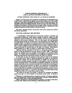
2.1. Voronoi Cell Finite Element Method (VCFEM). Around the 1990s, Ghosh and Mukhopadhyay [4] and Ghosh and Moorthy [5] proposed a technique to model and simulate polycrystalline ferroelectrics by using polygonal elements, which are formulated by using Voronoi cell. This method is known as Voronoi cell finite element method (VCFEM). The grains in the microstructure are represented by Voronoi cells, which are generated through Voronoi tessellation. Each of these Voronoi cells (in the form of polygons with arbitrary number of sides) contains heterogeneity (in the form of void or inclusions) and is treated as a single finite element. Figure 1 shows a Voronoi cell element with heterogeneity (within the element) and boundary conditions. The matrix phase is denoted as Ω𝑚 and heterogeneity phase as Ωℎ . The heterogeneity surface and element surface are denoted as 𝜕Ωℎ and 𝜕Ω𝑒 , respectively. The element boundaries consist of three types, which are prescribed traction/displacement boundary, free boundary, and interelement boundary. VCFEM combines assumptions from micromechanics theories and adaptive enhancements. This technique is computationally efficient compared to the conventional FEM (displacement based triangular or quadrilateral elements), since each polygonal grain is represented by a single finite element and no further subdivision of the domain is required. Stress functions for the interior of the element are obtained in terms of polynomial expansions of the global coordinates and these polynomial functions are formulated in such a way that they satisfy equilibrium within the element. An example of VCFEM formulation for analysis of Cosserat materials based on the parametric minimum complementary energy principle is given as [6] 𝑒

∏=∫ Ω

Ω

1 𝑇 𝑑𝜎 𝑆𝑑𝜎 𝑑Ω + ∫ 𝜆𝑇𝑄𝑑𝜎 𝑑Ω 2 Ω 𝑇

− ∫ 𝑑𝑇 𝑑𝑢 𝑑𝑠, 𝜕Ω

(1)

+ 𝛽9 𝑦3 + 𝛽13 𝑥4 + 𝛽14 𝑥3 𝑦 + 𝛽15 𝑥2 𝑦2 + 𝛽16 𝑥𝑦3

(2)

+ 𝛽17 𝑦4 + ⋅ ⋅ ⋅ Ψ = 𝛽4 𝑥 + 𝛽5 𝑦 + 𝛽10 𝑥2 + 𝛽11 𝑥𝑦 + 𝛽12 𝑦2 + 𝛽18 𝑥3 + 𝛽19 𝑥2 𝑦 + 𝛽20 𝑥𝑦2 + 𝛽21 𝑦3 + ⋅ ⋅ ⋅ ,

(3)

where 𝛽𝑖 (𝑖 = 1, 2, . . . 𝑛) are the undetermined coefficients. VCFEM has been found to perform poorly when the heterogeneity is in the form of voids (but works well for inclusions), due to the poorly defined stress functions within the interior of the element. This problem is solved by taking into account the geometry effects through conformal mapping [7]. Later, Sze and Sheng [8] included other characteristic features to the VCFEM by incorporating the electromechanical Hellinger–Reissner principle. Since then, the VCFEM has been revisited, extended, and implemented in different applications such as in analysis of heterogeneous materials [5, 9, 10], determination of the effective elastic properties/crack analysis of functionally graded materials [11, 12], analysis of microstructural Representative Volume Element (RVE) [13], simulation of the crack and analysis/failure analysis of composite materials [7, 14–19], and multiscale simulations for microstructural modelling [9]. The method is also extended to 3D [14, 20, 21]. Hybrid of VCFEM with other methods such as numerical conformal mapping (NCM) method can be seen in the work by Tiwary, Hu, and Ghosh [22]. The hybrid technique is known as NCM-VCFEM and it is developed so that real micrographs of heterogeneous materials with irregular shapes can be analyzed effectively. The effectiveness is attained by using NCM such as Schwarz–Christoffel mapping to convert arbitrary/irregular shapes of micrographs into a unit circle. Another example is coupling of VCFEM with parametric variational principle and the parametric quadratic programming method [6, 23]. This approach is implemented in order to incorporate the constitutive relations of the physical phenomenon and to generalize the variational

Mathematical Problems in Engineering

3 𝑢̃(1) represents the components of the specified displacements along 𝐶1 𝑠 represents boundary surface The interior stresses are obtained by using interpolation functions (in the form of trigonometric functions) through the following relation [25]:



y

r=1 b a C2

x



C1

𝜎 { 11 } { } 1 𝜎22 } = { { } 2𝜇 {𝜎12 } 2𝐶1 − 𝐶2 + 𝐶3 −2𝐷1 + 𝐷2 − 𝐷3 −𝐶1 𝐷1 [2𝐶 + 𝐶 − 𝐶 −2𝐷 − 𝐷 + 𝐷 𝐶 −𝐷 ] ⋅ ∑ [ 1 2 3 1 2 3 1 1]

Figure 2: Mapping of a Voronoi cell element.

𝑚𝑢

𝑘=𝑚𝑏

principle. The new formulations are found to be able to produce good solutions, competitive with that of conventional FEM package in ANSYS and with fewer nodes (which reduces the computational cost). Simultaneously, Zhang et al. [23] developed a polygonal finite element by using similar approach and named it as parametric variational principle based polygonal finite element method (PFEM). PFEM is similar to conventional displacement based finite elements in the sense that PFEM is applicable for macroanalysis and compatible interpolation functions are used for the entire element domain (boundaries as well as interior of the elements). VCFEM is generally suitable for micromechanical analysis and multiscale modelling [24].

[

𝐷2 − 𝐷3

𝐶2 − 𝐶3

𝐷1

𝐶1 ]

{𝑎̃𝑘 } { } { } { } { {𝑎̂𝑘 } } ⋅ { }, ̃ { 𝑏𝑘 } } { { } { { } } ̂𝑏 { 𝑘}

where 𝐶1 to 𝐶3 and 𝐷1 and 𝐷3 are the functions of 𝑘, 𝑟, and 𝜃. 𝑚𝑢 and 𝑚𝑏 are the upper and low limits of the series. 𝑟 and 𝜃 are the parameters that resulted due to the mapping of the computational/matrix region Ω to the elliptical region in reference system. Expression for 𝐶1 is shown here as an example: 𝐶1 (𝑘, 𝑟, 𝜃)

2.2. Hybrid Polygonal Element (HPE). On the other hand, Zhang and Katsube [25] proposed a different method to analyze micromechanical properties of heterogeneous materials. The authors used the hybrid stress element method [26] with Muskhelishvili’s complex analysis approach to formulate polygonal elements. This method is known as the hybrid polygonal element (HPE) method [27] and this technique is pursued, since the stress variation around the heterogeneity (inclusions) is not well defined in the VCFEM [28]. Knowing this, HPE has later been incorporated into VCFEM as well [20]. In the HPE method, the compatible interpolation functions are formulated along the boundaries only, while the interior of the element is represented by self-equilibrating stress field. Figure 2 shows a HPE in global 𝑥-𝑦 coordinate system and its equivalent mapping to a standard ellipse in reference 𝜂-𝜉 coordinate system. An example of a hybrid functional ∏(𝐻) 𝑒 for a HPE with hole (void) is given as [25] (𝐻)

∏= 𝑒

1 (∮ 𝑇𝑇 𝑢 𝑑𝑠 − ∮ 𝑇𝑇 𝑢 𝑑𝑠) − ∮ 𝑇𝑇𝑢̃(1) 𝑑𝑠, 2 𝐶1 𝐶2 𝐶1

(4)

where 𝑢 and 𝑇 are the matrices for displacement and traction components along the element 𝐶1 and 𝐶2 represent the element’s outer boundary with adjacent elements and the inner interface between the matrix and heterogeneity, respectively

(5)

= 𝑘𝑟𝑘−1 (𝑓1 cos (𝑘 − 1) 𝜃 − 𝑓2 sin (𝑘 − 1) 𝜃) ,

(6)

where 𝑓1 and 𝑓2 are functions in terms of 𝑟, 𝜃, 𝑎, and 𝑏. 𝑎 and 𝑏 represent the major and minor semiaxes of the mapped ellipse. Similar functions are used to determine the displacements within the element. Application of HPEs for the analysis of heterogeneous media in 2D as well as 3D can be seen in works by Zhang and Katsube [25] and Kaliappan and Andreas [29]. Wachspress shape functions were not utilized in these elements (in HPE and VCFEM), due to the difficulties in integrating the complex rational functions [28]. A limitation of the VCFEM and HPE methods is that the resulting polygonal elements can contain only one irregular phase (void/inclusion) within the element. Due to this, the extended multiscale finite element method [30] has been developed to analyze mechanical behaviors of heterogeneous materials with randomly distributed polygonal microstructure. Another version of HPE for plane linear elasticity problems with better performance compared to conventional FEM is presented in [31]. The polygonal meshes are generated based on the MATLAB code PolyMesher which operates based on Voronoi diagrams. 2.3. Conforming Polygonal Finite Element Method Based on Barycentric Coordinates (Conforming PFEM). Around the year of 2000, the Wachspress method gained more attention and was revisited alongside with other techniques to formulate interpolation or shape functions for polygonal

4 elements. These techniques are known as barycentric coordinates method [32, 33] and they yield complex shape functions consisting of rational, logarithmic, and trigonometric functions. Recently, polynomial spline functions (Bernstein Bezier functions) have been proposed to be included in the barycentric coordinates method [34]. Polygonal elements which are formed by these methods are implemented in FEM and known as conforming polygonal finite element method (conforming PFEM, or simply PFEM). Some of the barycentric coordinates methods used in the formulation of conforming PFEM are inverse bilinear coordinates [35], Wachspress [32, 36–40], mean value coordinates [41, 42], harmonic coordinates [43], maximum entropy coordinates [44–46], metric coordinates [47], and natural neighbor-based coordinates (Laplace shape functions) [33]. Some of the methods such as Wachspress, mean value, and harmonic coordinates have been extended to 3D [48–52]. The above mentioned barycentric coordinate methods are described below. Inverse bilinear coordinates were developed for quadrilaterals, based on bilinear mapping of a unit square to convex quadrilaterals. Rational functions are used for the mapping and their inverses were studied to develop the inverse bilinear coordinates for quadrilaterals. Wachspress developed rational polynomial functions which can be used to produce conforming shape functions for arbitrary polygons. Meyer et al. [32] modified the Wachspress coordinates by replacing the adjoint with triangle areas and rewrote the barycentric coordinates in a simpler form. Similarly, other simplifications were carried out onto the Wachspress coordinates such as representing the Wachspress coordinates in terms of perpendicular distance between two points [32], redefining the adjoint polynomials by other means [48], and so on. Advantages of Wachspress coordinates over inverse bilinear coordinates are that the Wachspress method is applicable for arbitrary polygons and do not contain square root terms [35]. However, Wachspress’ rational shape functions do not perform well for concave polygonal elements. This shortage is avoided in mean value coordinates, which are written in terms of trigonometric functions. Mean value coordinates can be adapted to complex arbitrary polygons, especially star-shaped geometries (concave polygons). It is noted that shape functions for concave polygonal elements cannot be represented by rational polynomial functions, since convex shapes (can be represented by rational polynomial functions) cannot be mapped to concave shapes [47]. Mean value coordinates are useful and vastly applied in parameterizing triangular meshes and surface fitting [35]. These barycentric coordinates are found to be robust and applicable for concave polygons as well, even though the method does not guarantee positive functions for all the cases, since it is bounded only for star-shaped geometries [47]. On the other hand, apart from being linearly precise, harmonic and maximum-entropy coordinates are guaranteed positive for both convex and concave polygons [46]. Another suitable barycentric coordinate which satisfies the boundedness requirement for both convex and concave polygonal elements is the metric coordinate method [53]. A general framework to construct barycentric coordinates was proposed by Floater,

Mathematical Problems in Engineering Hormann, and Kos [54]. This framework reproduces the barycentric coordinates under various values of coefficient 𝑐 in the formulation. Motivated by mesh-free method, authors of references [33, 47] developed natural neighbor-based coordinates (also known as Laplace shape functions) for arbitrary polygonal elements. The development is based on natural neighborbased schemes within a Voronoi cell. The method was later tested for utilization in FEM, together with Wachspress, metric, and mean value coordinates. Simulation results showed that the Laplace interpolant is simpler and computationally attractive and yields more accurate results compared to the rest for convex and weakly convex polygonal elements. Nonetheless, the Laplace interpolant is not suitable for concave elements and best results for convex elements are attained through mapping of parent element [33, 47]. Polygonal elements based on barycentric coordinates have been implemented in various areas such as computer graphics, animation and geometric modelling [55, 56], topology optimization [57], surface parameterization [58], geometric modelling [41], analysis of a plate with a circular hole [59], crack growth modelling [60], contact-impact problems [61], mesh generation, material fracture [62], finite elasticity problems [63], modelling of rock materials [64], and so on. Recently barycentric coordinates have been implemented in static and free vibration analyses of laminated composite plates [65], multimaterial topology optimization [66], Reissner-Mindlin plate problems [67], and transient heat conduction problems [68]. Other barycentric coordinates methods have been investigated such as Poisson coordinates [69], Green coordinates, reconstructions of Green coordinates by using Cauchy’s theorem, moving least squares coordinates, and attempt to design new methods through complex representation of real-valued barycentric coordinates [35]. However, evaluation of barycentric coordinates is neither simple nor efficient compared to the conventional displacement based FEM, due to the complex functions which arise in the former techniques. Furthermore, barycentric coordinates are not efficient for assembling the stiffness matrices associated with weak solutions of Poisson equations [34]. Construction of shape functions 0𝑗 based on Wachspress [47] for a polygonal element in the 𝑥-𝑦 coordinate system according to Figure 3 is given as

0𝑗 (𝑥, 𝑦) =

𝑤𝑗 (𝑥, 𝑦) =

𝑤𝑗 (𝑥, 𝑦) , 𝑛 ∑𝑘=1 𝑤𝑘 (𝑥, 𝑦) 𝐴 (𝑝𝑖 , 𝑝𝑗 , 𝑝𝑘 ) 𝐴 (𝑝, 𝑝𝑖 , 𝑝𝑗 ) 𝐴 (𝑝, 𝑝𝑗 , 𝑝𝑘 )

(7) ,

where 𝐴 represents area enclosed by the three nodes within the bracket 𝑃𝑖 , 𝑃𝑗 , and 𝑃𝑘 represent a particular external/surface node of the polygonal element 𝑃 represents inner node of the polygonal element


5 3

Pk 4 s4

Pj

ΨＤ

s3 h4

Ｄ

h3

s2

h2

5

P

2

h5

s5

h6

h1 s1

s6

1

Pi 6

Figure 3: Construction of shape functions based on Wachspress.

Figure 5: Construction of shape functions based on the concept of natural neighbors.

Pk 3

j j

P

4

Pj

Ωsk

i

j i

5

2

0

i Pi 1

Figure 4: Construction of shape functions based on mean value coordinates.

The expression for 𝑤𝑗 (𝑥, 𝑦) in (7) can be rewritten by using the angles formed (𝜑 and Ψ) between the nodes [47] as 𝑤𝑗 (𝑥, 𝑦) = 2 (

cot𝜑𝑗 + cotΨ𝑗 2

2

(𝑥 − 𝑥𝑗 ) + (𝑦 − 𝑦𝑗 )

)

(8)

The expression for 𝑤𝑗 (𝑥, 𝑦) in (7) based on mean value coordinates [47] for a polygonal element is given as 𝑤𝑗 (𝑥, 𝑦) =

tan (∝𝑖 /2) + tan (∝𝑗 /2) 2

√(𝑥 − 𝑥𝑗 ) + (𝑦 − 𝑦𝑗 )

2

,

(9)

where ∝ is the angle that is formed within the triangular partitions at the inner node, as shown in Figure 4. The expression for 𝑤𝑗 (𝑥, 𝑦) in (7) based on the concept of natural neighbors (Laplace shape functions) [47] for a polygonal element according to Figure 5 is given as 𝑤𝑗 (𝑥, 𝑦) =

𝑠𝑗 (𝑥, 𝑦) ℎ𝑗 (𝑥, 𝑦)

where 𝑠𝑗 represents length of the Voronoi edge and ℎ𝑗 2

2

√(𝑥 − 𝑥𝑗 ) + (𝑦 − 𝑦𝑗 ) .

6

Figure 6: Partitioning of a nSFEM element into subtriangles.

2.4. 𝑛-Sided Polygonal Smoothed Finite Element Method (nSFEM). Another attempt to form polygonal finite element method can be seen within the smoothed finite element method (SFEM). SFEM is formed by merging conventional FEM with meshless methods. SFEM was initially formed for quadrilateral elements. Later, Dai, Liu, and Nguyen [70] extended the four-node quadrilateral smoothed elements to arbitrary sides termed as n-sided polygonal smoothed finite elements (nSFEM) and implemented the method in solid mechanics (macrolevel). In nSFEM, the polygonal element is divided into several smoothing cells in the form of triangles, which share a common node at the center of the polygon. These triangles known as smoothing cells are then subjected to smoothing techniques onto the strain components. An example of nSFEM element is shown in Figure 6. Point 0 in Figure 6 represents the center of the polygonal element. The displacement at this point, 𝑑0 is taken as the average of displacement of all the external nodes, given by the following equation [71]:

(10) 𝑑0 = =

1 𝑛 ∑𝑑 , 𝑛 𝑝=1 𝑝

(11)

where 𝑑𝑝 represents displacement at a particular node 𝑝 and 𝑛 represents total number of nodes of the polygon. The

6


displacement within a particular subtriangle 0-1-6 (subtriangle 1) can then be represented by [71]: 𝑢𝑖,1 = 𝑁1 𝑑1 + 𝑁2 𝑑2 + 𝑁3 𝑑0 ,

(12)

where 𝑁𝑗 (𝑗 = 1, 2, 3) represents the conventional shape functions for a 3 nodes’ triangular element. Substituting (12) into (11) and simplifying gives 1 1 1 𝑢𝑖,1 = (𝑁1 + 𝑁3 ) 𝑑1 + (𝑁2 + 𝑁3 ) 𝑑2 + 𝑁3 𝑑3 𝑛 𝑛 𝑛 1 1 + ⋅ ⋅ ⋅ + 𝑁3 𝑑𝑛−1 + 𝑁3 𝑑𝑛 𝑛 𝑛

D

C

Ωsk

K

0

(13)

The shape function matrix for subtriangle 0-1-6 then becomes Figure 7: Smoothing domain Ω𝑠𝑘 (OCDKO) for nES-FEM.

𝑁 1 1 1 1 1 = {(𝑁1 + 𝑁3 ) (𝑁2 + 𝑁3 ) ( 𝑁3 ) ⋅ ⋅ ⋅ ( 𝑁3 ) ( 𝑁3 )} 𝑛 𝑛 𝑛 𝑛 𝑛

(14)

The strain components are smoothed according to [71] 𝑛

𝜀 (𝑥) = ∑𝐵𝐼 (𝑥, 𝑦) 𝑑𝐼

(15)

𝐼=1

𝐵𝐼 (𝑥, 𝑦) =

1 ∫ 𝐵̃ (𝑥, 𝑦) 𝑑Ω, 𝐴𝑠𝑘 Ω𝑠𝑘 𝐼

(16)

where 𝐴𝑠𝑘 represents area of smoothing domain, 𝐵̃𝐼 represents the conventional compatible strain displacement matrix, and Ω𝑠𝑘 represents the smoothing domain. There are three types of smoothing techniques applicable for these smoothing cells, which are cell, node, and edge based. These techniques are known as n-sided polygonal cellbased smoothed FEM (nCS-FEM) [70], n-sided polygonal edge-based smoothed FEM (nES-FEM) [72], and n-sided polygonal node-based smoothed FEM (nNS-FEM) [73, 74], respectively. In case of nCS-FEM, the smoothing is carried out by integrating the gradient of displacement over the particular smoothing cell’s triangular area (for 2D as shown in Figure 6), individually [71]. When combined with the conventional FEM to obtain the displacements, the area integration is reduced to surface integration for the case of a constant smoothing function. The smoothed stiffness matrix for an element is then obtained by summing up individual stiffness matrices of all the smoothing cells within the polygonal element. Shape functions are derived for each side/edge of the smoothing cells by using the two nodes that make up the particular side/edge. These shape functions for the sides/edges should be compatible, since these sides coincide with each other to form the polygonal element. Shape functions for the interior of the smoothing cells are obtained by using other methods such as PFEM or mesh-free techniques [70]. In case of nES-FEM, the smoothing is done based on particular edge/side (instead of cell as in nCS-FEM) of the smoothing cells within the polygonal element as shown in Figure 7. The smoothing is done by performing the integration over several cell domains which are linked to the particular edge or side.

D Ωsk

E

F

C

B A

Figure 8: Smoothing domain Ω𝑠𝑘 (ABCDEFA) for nNS-FEM.

Therefore, the integration domain may extend to smoothing cells of adjacent elements as well (since a particular side/edge can be shared by adjacent elements) [71]. In case of nNSFEM, the smoothing is done based on a particular node of the smoothing cells within the polygonal element as shown in Figure 8. Similarly, the smoothing is done by performing the integration over several cell domains which are linked to the particular node and therefore, the integration domain may also extend to smoothing cells of adjacent elements (since a particular node can be shared by adjacent elements) [71]. nCS-FEM has many advantages over the conventional FEM such as the fact that stability provides accurate results as compared to the conventional FEM. This is because the stiffness matrices of nCS-FEM tend to be less stiff and can be applied for nearly incompressible materials by using selective integration schemes to avoid volumetric locking phenomena [70]. However, for solid mechanics, nCS-FEM is proposed to be used only for regions near the boundary or very irregular parts. This is because use of these elements for interior regions would increase the number of nodes and

Mathematical Problems in Engineering s

3 4

(x2 , y2 ) 2 s=1

Line element 0 5

Similar curve for  = 0.5

6

=1

2.5. Polygonal Scaled Boundary FEM (PSBFEM). Scaled boundary FEM is a semianalytical method which combines the boundary element method (BEM) and FEM. It was first introduced by Song and Wolf [81], and it was soon extended to polygonal elements and named as Polygonal Scaled Boundary FEM (PSBFEM). Example of a PSBFEM element is shown in Figure 9. PSBFEM works based on scaling center, which is located at the center of the polygonal element. The scaling center is located within the polygonal element (usually at the center) in such a way that all the boundaries/sides of the polygonal element are visible from this scaling center. Radial lines are formed from the scaling center to the outer nodes of the polygonal element, and these lines are assigned value of zero at the center (scaling node) and reach value of 1 at each node. This is accomplished through implementation of radial coordinate system. Similarly, each boundary/side of the polygonal element is assigned value of 1 to -1, through implementation of local coordinate system. The boundaries are represented by conventional numerical line elements of FEM.

Radial line

 = 0.5

eventually increases the computational cost [70]. Advantage of nNS-FEM is that it is immune from volumetric locking phenomena. Disadvantage of nNS-FEM is that the computational time is longer compared to conventional FEM for the same number of global nodes, due to larger bandwidth of stiffness matrices. Disadvantage of nES-FEM is that there is a tendency to overestimate or underestimate the strain energy of the model for some cases. Apart from that, similarly to nNS-FEM, nES-FEM requires more computational time compared to conventional 3-node triangular elements due to the larger bandwidth [72]. Comparison between the three types of nSFEM is provided by Nguyen et al. [72], for solid mechanics problem. It is shown that nES-FEM provides most accurate solution compared to the others and the stiffness/softness of the model of nES-FEM is in between the other two techniques. Combination of nES-FEM and nNSFEM (termed as nES/NS-FEM) to avoid volumetric locking and to achieve faster convergence can be seen in the literature [72, 75]. Applications of nSFEM can be seen in determination of upper bound solutions to solid mechanics problems [73], fluid-solid interaction problems [75], and new application in analysis of elastic solids subjected to torsion [76]. Recently, nSFEM has been implemented for the analysis of fluidsolid interaction (FSI) problems in viscous incompressible flows together with sliding mesh [77]. Simulation results showed that the method performs better compared to the conventional finite elements. Major advantage of the nSFEM in FSI is that it is capable of performing independent domain discretization. Generally, the nSFEM is advantageous over the conventional FEM since it produces more accurate solutions, able to tolerate volumetric locking and does not require isoparametric mapping (which enables the elements to take arbitrary shape: concave and convex forms). Apart from that, the shape functions consist of polynomials, which are easier to evaluate compared to the conforming PFEM based on barycentric coordinates. Extension of the method to 3D can be seen in literatures [78–80].

7



1 s = -1 (x1 , y1 ) Scaling center

Figure 9: A PSBFEM element.

Solution along the radial direction is obtained by analytical expressions by using m number of shape functions, where m represents number of nodes of the polygonal element. Transformation between the Cartesian coordinates and scaled boundary coordinates (radial coordinate system and local coordinate system) is accomplished through isoparametric mapping similar to the conventional FEM. The mapping which describes scaling of the boundary has led to the name of the method. Equation (17) [82] shows transformation of coordinate system (transformation between the scaled boundary coordinate system 𝜉, 𝑠 and Cartesian coordinate system x, y) for a point within the triangular subdomain 0-1-2 (as shown in Figure 9). Similar transformation is done for any point within any particular triangular subdomain. 𝑥 = 𝜉 [𝑁 (𝑠)] {𝑥𝑏 } 𝑦 = 𝜉 [𝑁 (𝑠)] {𝑦𝑏 } ,

(17)

where 𝑁(𝑠) = [ 𝑁1 (𝑠) 𝑁2 (𝑠) ] = [ (1/2)(1 − 𝑠) (1/2)(1+ 𝑠) ] represents shape functions of the line element and {𝑥𝑏 } = 𝑦 { 𝑥𝑥12 } and {𝑦𝑏 } = { 𝑦12 } represent the coordinates of the boundary nodes enclosed by the specific triangular subdomain (subdomain 0-1-2). The displacement 𝑢(𝜉, 𝑠) within a particular triangular subdomain of the element is interpolated through utilization of similar shape functions as shown in (18) below [82]: 𝑢 (𝜉, 𝑠) = [𝑁 (𝑠)] {𝑢 (𝜉)} ,

(18)

where 𝑢(𝜉) = { 𝑢𝑢12 (𝜉) (𝜉) } represent the displacements on the lines (radial lines) passing through the scaling center, 0, and nodes 1 and 2, respectively. Various applications of PSBFEM can be seen in literature such as in linear elasticity [83], crack propagation [84–88], applications within geotechnical structures [89], dynamic fracture simulation [90], analysis of cracked functionally graded materials [91], polygonal mesh creation (Song et al., 2017), elastoplastic analysis of structures [92], prediction of structural responses with randomly distributed material properties [93], simulation of crack surface contact problems

8


[94], and analysis of mesoscale concrete samples [95]. Extension of the method to 3D can be seen in the literature [96–98]. Advantages of PSBFEM compared to BEM and conventional FEM are that, in PSBFEM, analytical solutions are achieved inside the domain, discretization of free and fixed boundaries and interfaces between different materials are not required, and the calculation of stress concentrations and intensity factors based on their definition is straightforward [82]. PSBFEM exhibits some disadvantages [82]. PSBFEM is not directly applicable for unbounded domains with strongly inclined interfaces, due to the difficulty in selecting a scaling center within the body which is visible to all sides of the domain. Some modifications are needed for these cases such as the introduction of redundant nodes for subdomain creation or by moving the boundaries upward in order to create a single scaling center (alteration of the actual physical problem). In case of time dependent problems, PSBFEM cannot be directly used to process transient excitation as opposed to BEM. Unit impulse response matrices are required and there is a need for convolution integrals which increases the computational effort. It is also found that this method is not as efficient as conventional FEM or BEM when solving problems involving smooth stress variations within bounded/enclosed domain. However, PSBFEM yields highly accurate solutions for problems involving stress singularities. The stress singularity refers to a particular point within the domain in which the stress does not converge to a specific value. PSBFEM has been found to be superior to other techniques such as nSFEM and conforming PFEM within the context of linear elasticity and the linear elastic fracture mechanics [83]. 2.6. Mimetic Finite Difference (MFD) Method and Virtual Element Method (VEM). One of the difficulties faced in the construction of polygonal finite elements is the development of interpolation functions which extends to the interior of the element. Beir ao da Veiga, Gyrya, Lipnikov, and Manzini [99] implemented a mimetic finite difference (MFD) method to polygonal mesh and showed that the method is efficient in solving problems involving polygonal meshes, since the method uses only the surface representation of discrete unknowns and therefore the formulations are simpler. For example, consider a heat conduction phenomenon which is governed by the following governing equation (19) [100]: −div (𝐾∇𝑢) = 𝑞,

(19)

where K represents the full conductivity tensor, u represents the temperature, and q is the forcing term indicating the source of heat. The crucial step in MFD method is to mimic the essential properties of the physical and mathematical model above, which can be achieved through Green formula: → 󳨀 → 󳨀 ∫ 𝐾−1 (𝐾∇𝑢) ⋅ 𝐹 𝑑𝑥 = − ∫ 𝑢 div 𝐹 𝑑𝑥 Ω

Ω

→ 󳨀 󳨀 𝑛 𝑑𝑥, + ∫ 𝑢0 𝐹 ⋅ → 𝜕Ω

(20)

Figure 10: Low order degrees of freedom for MFD method. The arrows represent fluxes and the center represents the temperature.

→ 󳨀 where 𝐹 represents the heat flux. Subsequent step is implementation of the finite difference discretization, which involves discretization of scalar functions, vector functions, and the differential operators div and 𝐾∇. Discretization of scalar and vector functions is accomplished through introduction of degree of freedom. Example of degrees of freedom for low order MFD method is shown in Figure 10. An additional step is necessary, which is the discretization of the integrals. This step is required in order to approximate div and 𝐾∇ (differential operators) according to mimetic approach. The method is also shown to be useful for meshes with degenerate and nonconvex polygonal elements. Since then, MFD method has been implemented in various problems (diffusion/convection-diffusion [101–104], electromagnetic field problems [105, 106], elasticity problems, Lagrangian hydrodynamics problems [107], and solving wave equations [108]) and for modelling fluid flows [109, 110]. MFD has been extended to higher order [100, 102] and also to 3D [102, 105, 111, 112]. Beir ao Da Veiga, Brezzi, Cangiani, Manzini, Marini, and Russo [113] mentioned that it was quite difficult to present MFD due to nonexistence of trial functions for the interior of the element. Therefore, the MFD has been generalized and reintroduced as virtual element method (VEM). In VEM, the unknown degrees of freedom are attached to trial functions within the interior of the polygonal domain (which do not exist earlier in MFD). Three variants of VEM are presented by Russo [114], with different number of these internal degrees of freedom. This approach is now similar to conventional PFEM. This similarity opened the possibility of coupling VEM with the conforming PFEM. The resulting hybrid method (VEM-PFEM) has been found to possess high accuracy and, most importantly, the difficulties faced in the integration of complex functions resulting from barycentric coordinates in PFEM are entirely avoided [62]. Applications of VEM [115] can be seen in plate bending problems, elasticity problems, Stokes problems, Steklov eigenvalue problems, finite strain plasticity problems [116], hyperbolic problems [117], and topology optimization problems [118]. Extension of VEM to 3D can be seen in literatures [119, 120].


9 3

The virtual element space on a polygonal domain (that discretizes the problem domain) is defined as [113]

4 T3

𝑉𝐾,𝑘 = {V ∈ 𝐻1 (𝐾) : V|𝜕𝐾 ∈ B𝑘 (𝜕𝐾) , 󳵻V|𝐾 ∈ P𝑘−2 (𝐾)} ,

T4

(21) 5

2

T2 7

T1

T5

where 𝑉𝐾,𝑘 represents the finite dimensional space, K represents a generic polygonal element within the domain, k represents polynomial degree of the virtual element scheme, V represents displacement field, 𝐻1 (𝐾) represents the space containing K, 𝜕𝐾 represents a generic edge on the polygon, B𝑘 (𝜕𝐾) represents the set of polynomials of degree less than or equal to k on 𝜕𝐾, and P𝑘−2 (𝐾) denotes the space of polynomials of degree less than or equal to k-2 on K. For k = 1, the trial functions are linear on each edge and the inside of the element is represented by harmonic functions. For k = 2, the trial functions on each edge are made of polynomials of degree less than or equal to 2. The inside of the element is composed of polynomials with constant Laplacian. A similarity between VCFEM, HPE, MFD, and VEM is that these methods do not require the extension of compatible interpolation functions to the interior of the element. The compatible interpolation functions are required for the element boundaries only, which simplifies the formulation and enables the formulation of elements with arbitrary number of sides/nodes. Disadvantage of MFD and VEM is that they involve complex procedures and therefore require high computational effort [121]. 2.7. Virtual Node Method (VNM). Another attempt to overcome the difficulty in forming compatible shape functions for polygonal FEM can be seen in the literature [122]. The authors presented a novel polygonal FEM which uses a virtual node at the center of the element to formulate shape functions consisting of simple polynomials. The method was proposed as an alternative to the conforming PFEM which suffered from inaccuracy resulting from the integration of complex functions in the stiffness matrix. First, a polygonal element with arbitrary number of nodes is formed. The polygonal domain is then divided into several triangular regions, which share a common node at the center of the element (denoted as the virtual node), as shown in Figure 11. Compatibility among each triangular region is fulfilled by using the conventional FEM shape functions of a 3 nodes’ triangular element. These triangular regions are then coupled together (to form the polygonal element) by representing the virtual node at the center in terms of mean least square shape functions, as shown by (22) [122, 123]:

T6 1 6

Figure 11: Partitioning of a polygon according to VNM.

𝑇1 (an example), 𝑇V = 𝑇1 , 𝑖 = 1, 𝑗 = 2, and 𝑘 = 7. Equation (22) above can be written as 𝜑 = 𝜙𝑖 𝜑1 + 𝜙𝑗 𝜑2 + 𝜙𝑘 𝜑̂7

(23)

Field variable at the internal node (virtual node) 𝜑̂7 can be represented by the least mean square [123]: 𝑛

𝜑̂7 = ∑ 𝑁𝑚 𝜑𝑚 = 𝑁𝑇𝜑,

(24)

𝑚=1

where 𝑛 represents total number of nodes of the polygonal element, 𝑁𝑇 = 𝑝𝑇 (𝑥, 𝑦)𝐴−1 𝐵, 𝑝 is a set of basis functions, and 𝐴 and 𝐵 are basis matrices. Equation (24) can be rewritten in terms of shape function for a particular node: [𝑇V ]

[𝑇V ] 𝜙𝑚 = (𝜙𝑖

[𝑇 ]

+ 𝜙𝑗 V )

[𝑇V ] 󸀠 𝜑𝑖

⋅ [(𝜙𝑖

[𝑇 ]

[𝑇 ]

+ 𝜙𝑗 V 𝜑𝑗󸀠 ) + 𝜙𝑘 V 𝑁𝑚 (𝑥𝑘 , 𝑦𝑘 )]

[𝑇 ]

+ 𝜙𝑘 V 𝑁𝑚 𝜑𝑖󸀠

(25)

{1, 𝑖𝑓 𝑚 = 𝑖, ={ 0, 𝑖𝑓 𝑚 ≠ 𝑖; {

{1, 𝑖𝑓 𝑚 = 𝑗, 𝜑𝑗󸀠 = { 0, 𝑖𝑓 𝑚 ≠ 𝑗. { Stiffness matrix for a particular polygonal element is obtained by summing up stiffness matrices of the individual triangular regions. Next, global stiffness matrix is obtained by summing up all the stiffness matrices of the individual polygonal elements. These are shown by (26) and (27) below: 𝑛

[𝑇V ]

𝜑

=

[𝑇 ] 𝜙𝑖 V 𝜑𝑖

+

[𝑇 ] 𝜙𝑗 V 𝜑𝑗

+

[𝑇 ] 𝜙𝑘 V 𝜑̂𝑘 ,

(22)

where 𝜑 represents unknown field variable at a particular point/node, 𝜑̂ represents the field variable at the virtual node, 𝜙𝑖 , 𝜙𝑗 , and 𝜙𝑘 are the conventional FEM shape functions of a 3 nodes’ triangular element, and 𝑇V represents a particular triangular element within the polygonal domain. For triangle

𝑘𝑒 = ∑ 𝑘𝑇V

(26)

V=1 𝑙

𝐾 = ∑ 𝑘𝑒 ,

(27)

𝑒=1

where l represents total number of elements in the mesh. It can be seen that this method is quite similar to nCS-FEM

10


in terms of the partitioning of the domain into triangular regions/cells, integration is performed on each triangular region/cell individually, and summing of stiffness matrices of each triangular region/cell to obtain the element stiffness matrix. The difference is that strain smoothing is not carried out in VNM. The method is later extended to higher order by Oh and Lee [124]. The method is advantageous compared to compatible PFEM due to the simple polynomial shape functions (which is easier to work with). VNM is found to be efficient in adaptive computation, by using quadtree or octree mesh. The method has been extended to 3D polyhedral (VPHE) and hexahedral forms and implemented in adaptive computations as can be seen in the literature [123, 125, 126]. Recently, the method has been coupled with extended FEM (XFEM) [127, 128]. 2.8. Discontinuous Galerkin FEM (DGFEM). This method was proposed due to the difficulties faced in executing other polygonal FEMs such as compatible PFEM, MFD, and VEM. The difficulties arise due to the complicated shape functions in compatible PFEM and complex procedures involved in MFD and VEM. These complicated entities demand high computational effort as well [121]. DGFEM, on the other hand, does not require any conforming shape function and the method is simple. Application of DGFEM in polygonal meshes can be seen in the literature [129–135]. Extension of the method to 3D can be seen in the literature [136, 137]. In DGFEM, the problem domain is discretized into several polygonal cells which represent the polygonal elements. The interpolation for the elements is carried out based on a set of monomial functions which are totally independent of the element. These interpolation functions do not comply to shape function requirements of conventional FEM and therefore they are not continuous across different elements (not compatible). Due to this, integrations are carried out on the boundaries of each cell. This step is an addition compared to the conventional FEM. The degrees of freedom are obtained based on the coefficients of the linear combination of the monomial functions [138]. Additional advantages of the method are that the adjacent elements can be of different order and the elements do not need to be conforming. Interpolation of field variables Θ within the element is achieved through [130] Θ = {𝑁} {Θ} ,

(28)

Θ1 Θ2 .. .

] represents matrix of the local degrees where {Θ} = [ 𝑁𝑒 [Θ ] of freedom, Ne represents the number of polygonal elements, {𝑁} = [𝑠1 𝑏1 𝑠2 𝑏2 . . . 𝑠𝑁𝑒 𝑏𝑁𝑒 ] represents matrix containing the incompatible interpolation functions b, and 𝑠 represents the element support [130]: {1 𝑓𝑜𝑟 𝑝𝑜𝑖𝑛𝑡 𝑤𝑖𝑡ℎ𝑖𝑛 𝑡ℎ𝑒 𝑑𝑜𝑚𝑎𝑖𝑛 𝑠={ 0 𝑓𝑜𝑟 𝑝𝑜𝑖𝑛𝑡 𝑜𝑢𝑡𝑠𝑖𝑑𝑒 𝑡ℎ𝑒 𝑑𝑜𝑚𝑎𝑖𝑛 {

The interpolation functions can be made of different kinds of functions. For instance, the functions can be polynomials which are obtained from Taylor expansion as shown below for various degrees [130]: First order: 𝑏 = [1 𝑥 𝑦] Second order: 𝑏 = [1 𝑥 𝑦 𝑥𝑦 𝑥2 𝑦2 ] 3rd order: 𝑏 = [1 𝑥 𝑦 𝑥𝑦 𝑥2 𝑦2 𝑥3 𝑥2 𝑦 𝑥𝑦2 𝑦3 ] where 𝑥 and 𝑦 are the local coordinates. The interpolation functions can also be made of radial basis functions [130]: 2

2

2

𝑏 = 𝑒−𝑟1 𝑒−𝑟2 ⋅ ⋅ ⋅ 𝑒−𝑟𝑛 ,

(30)

where 𝑟𝑖2 = (𝑥 − 𝑥𝑖 )2 + (𝑦 − 𝑦𝑖 )2 and (𝑥𝑖 , 𝑦𝑖 ) represents coordinates of the polygon vertices as well as the mass center. The stiffness matrix 𝐾 for a heat transfer phenomenon is obtained through the formula [130] 𝐾 = ∫ 𝑘𝐵𝑇𝐵 𝑑Ω Ω

𝑇

− ∫ 𝑘 ⟦𝑁⟧ 𝑛𝑠𝑇 ⟨𝐵⟩ 𝑑Γ + 𝜅 ∫ 𝑘 ⟨𝐵⟩𝑇 𝑛𝑠 ⟦𝑁⟧ 𝑑Γ Γ𝑠

(31)

Γ𝑠

𝑇

+ ∫ 𝜎 ⟦𝑁⟧ ⟦𝑁⟧ 𝑑Γ + ∫ 𝜎𝑁𝑇 𝑁𝑑Γ, Γ𝑠

ΓΘ

where ⟦𝑁⟧ represents discontinuity jump, ⟨𝐵⟩ represents mean value of 𝐵, Ω represents the domain space, B represents matrix containing the differentiation of interpolation functions, k represents thermal conductivity, 𝑛𝑠 represents unit vector which is tangent to the boundary, ΓΘ represents boundary of the polygon, ΓΘ represents boundary in which the unknown variable (temperature) is prescribed, 𝜎 represents discontinuity penalization parameter, and parameter 𝜅 has the value +1, -1, or 0, depending on the scheme. 2.9. Trefftz/Hybrid Trefftz Polygonal Finite Element (T-FEM or HT-FEM) and Boundary Element Based FEM (BEM-Based FEM). T-FEM utilizes two different sets of functions to approximate the solutions, one for the boundary and the other is for the interior domain. For the interior of the element, a series of homogeneous solutions of the governing equation (problem equation to be solved) is used as basis functions. These basis functions are known as T-complete set and they are not conforming across the element boundaries [139]. The boundary is represented by other independent sets of conforming basis functions. An example of T-FEM element is shown in Figure 12. The displacement 𝑢 within a domain (interior) can be interpolated by using 𝑚

𝑢 = 𝑢̌ + ∑𝑁𝑖 𝑐𝑖 ,

(32)

𝑖=1

(29)

where 𝑢̌ represents the known function on the boundary, 𝑁𝑖 is the trial function, 𝑐𝑖 is the unknown coefficient, and


11 m

3

u = ǔ + ∑ Ni ci

4

3

10

9

i=1

4

2

11

2

5 5

 u = N(x)d

8 12

y 1 x 6

j i 6  = -1

7 =0

k



1  = +1

Figure 13: An example of a HS-F element.

Figure 12: An example of T-FEM with its shape functions utilized for the case of solid mechanics.

m represents number of trial functions. The trial functions 𝑁𝑖 can be generated from Muskhelishvili’s complex variable formulation [139]. The displacement 𝑢̃ on the boundary of the domain can be interpolated by using (33) below: ̃ (𝑥) 𝑑, 𝑢̃ = 𝑁

(33)

where 𝑑 represents vector of nodal displacements and ̃ 𝑁(𝑥) = { (1−𝜉)/2 (1+𝜉)/2 represents matrix of the corresponding onedimensional shape functions for the boundary in terms of the local coordinate system, 𝜉. Continuity or boundary conditions are incorporated into the interior domain by various ways, in which one of the ways is by hybrid method known as hybrid Trefftz finite element method (HT-FEM). This method uses the conforming functions of the element boundary (also known as frame) to link the interior of the elements together [140]. HT-FEM has been successfully applied in linear elasticity problems [140] and found to be able to produce more accurate results and higher convergence rates compared to the conforming PFEM with Laplace/Wachspress shape functions. One of the advantages of the HT-FEM is that elements with embedded cracks or voids can be constructed. This leads to the development of new VCFEMs for microstructural analysis. The new method is known as T-Trefftz Voronoi Cell Finite Elements (VCFEM-TTs) [141] and was soon extended to 3D [142]. Recently another novel hybrid FEM has been formulated, by coupling HT-FEM with the idea of the Method of Fundamental Solution (MFS) known as hybrid fundamental solution based FEM (HFS-FEM) [143]. The advantage of HT-FEM compared to conventional FEM [144] is that this method is able to handle geometry induced singularities and stress/force concentrations efficiently without mesh adjustment. This is achieved by employing special purpose Trefftz functions that satisfy both the governing equations and boundary conditions associated with the singularities. Apart from that, general polygonal elements with curved sides can be generated and the elements are tolerant to mesh distortions. Advantages of HT-FEM compared to BEM [144] are that this method is applicable for problems involving different and heterogeneous materials, and boundary integration can be avoided when field variables are to be computed inside an element and the calculation of

coefficient matrices are simpler. Disadvantage of the method is that the T-complete set for some problems are either complex or difficult to formulate. Application of the method to 3D is described by Copeland, Langer, and Pusch [139]. Soon, another version of polygonal FEM emerged known as Boundary element-based FEM (BEM-based FEM) [139, 145– 148]. This method is developed based on the Trefftz function. 2.10. Hybrid Stress-Function (HS-F) Polygonal Element. Another method has been proposed by combining the principle of minimum complementary energy (similar principal used in VCFEM) with the Airy stress function which is known as hybrid stress-function (HS-F) element method. It was developed for quadrilaterals and triangles [149–154]. These elements are found to possess excellent performance compared to the conventional elements and especially independent of the element geometry (immune to mesh distortion). Later Zhou and Cen [155] expanded the method to polygonal elements. An example of HS-F polygonal element is shown in Figure 13. Nodes 1-6 are corner nodes and nodes 712 are the midside nodes. Local coordinate system 𝜉 is shown in Figure 13 for the edge 6-7-1. The displacement along a particular element edge d is given by [155] 𝑑 = 𝑁𝑞,

(34)

where 𝑁 = {𝑁𝑖 𝑁𝑗 𝑁𝑘 } represents the vector of shape functions for the three nodes (i, j, k) along a particular edge of the element and 𝑞 = {𝑢𝑖 V𝑖 𝑢𝑗 V𝑗 𝑢𝑘 V𝑘 } represents the displacement vector for the nodes. The shape functions are given as [155] 𝑁1 = −0.5𝜉 (1 − 𝜉) 𝑁2 = 1 − 𝜉2

(35)

𝑁3 = 0.5𝜉 (1 + 𝜉) , where 𝜉 represents local coordinate system along each element boundary. The element stress fields are given as [155] 𝜎 = 𝑆𝛽 + 𝜎∗ ,

(36)

where S is the stress solution matrix (with dimensions 3 by k) which is derived from k number of analytical solutions of the

12

Mathematical Problems in Engineering T

T

M

4

L

where 𝑇𝐼1 , 𝑇𝐼2 are the components of force vectors which act on the center of edge I, 𝑃𝐼1 , 𝑃𝐼2 are the components of position vector of point I, and A represents area of the element.

M

T

3

N

N

2

L

5 I K

T

I

1

y TK

J

6 x

T

J

Figure 14: An example of a BFEM element.

Airy stress functions, 𝛽 represents matrix (with dimensions k by 1) of unknown stress parameters and 𝜎∗ represents particular solution corresponding to body forces. 2.11. Base Forces Element Method (BFEM). Stress based FEMs such as HPE and HS-F are not well desired for most of the engineering applications, due to the difficulties in obtaining suitable/compatible stress functions. Furthermore, it is difficult to acquire nodal displacements in stress based FEMs [156]. BFEM on the other hand was formulated based on the concept of “base forces” which was introduced by Gao [157]. This method replaces the stress functions in the stress based FEMs with base forces which are easier to obtain (obtained directly from strain energy). Conventional FEM exhibits major drawback for nonlinear analysis. The conventional FEM is not able to approximate the strain and force fields accurately since these terms are dependent on the interpolation of the displacement field (displacement shape functions). This problem is avoided in BFEM which is directly based on interpolation of the internal force fields (force shape functions) [158]. Performance of BFEM is also found to be superior than conventional FEM when analyzing large strain contact problems and the nonlinear problems. This is because the deformation field in conventional FEM is complex and discontinuous near nonlinear regions and, in the case of large strain problems, the steep gradients of deformation cannot be represented accurately by the conventional shape functions [159]. BFEM has been later extended to polygonal elements based on the complementary energy principle [160] and potential energy principle [161]. Figure 14 shows an example of a BFEM element. 𝐼, 𝐽, 𝐾, 𝐿, 𝑀, 𝑁 represent the edges of the element and 𝑇𝐼 , 𝑇𝐽 , 𝑇𝐾 , 𝑇𝐿 , 𝑇𝑀, 𝑇𝑁 represent the force vectors which act on the element edges. The stresses corresponding to a point I on the element can be represented as [160] 4

4

[ ∑ 𝑇𝐼1 𝑃𝐼1 ∑𝑇𝐼1 𝑃𝐼2 ] ] 1[ 𝐼=1 𝐼=1 ], 𝜎= [ 4 4 [ ] 𝐴[ ] 𝐼2 𝐼2 ∑ 𝑇 𝑃𝐼1 ∑𝑇 𝑃𝐼2 𝐼=1 [𝐼=1 ]

(37)

2.12. Other Recent Techniques/Schemes. Recently, more new schemes have been proposed for the development of polygonal/polyhedral finite elements. They are the Compatible Discrete Operator (CDO) scheme [162, 163], Hybrid High-Order (HHO) scheme [164–166], Weak Galerkin (WG) scheme [167–171], gradient correction scheme [172], and vertex-based schemes [173]. Other recent techniques/methods include analysis of polygonal carbon nanotubes reinforced composite plates by using the first-order shear deformation theory (FSDT) and the element-free IMLS-Ritz method [174], an adaptive polygonal finite element method using the techniques of cut-cell and quadtree refinement [175], new adaptive mesh generation for polygonal element [176], and ultraweak formulations for high-order polygonal finite element methods [177]. New technique for 3-dimensional polyhedral elements can be seen within the framework of the finite volume method [178]. Another new approach to form polyhedral elements is by cutting a regular hexahedral element with CAD surfaces [179].

3. Comparison of the Various Methods Various techniques described in Section 2 above are compared with the recently proposed polyhedral element, known as Virtual Node Polyhedral Element, VPHE (threedimensional version of Virtual Node Method, as mentioned in Section 2.7 above). The comparison is given in Table 1.

4. Software Packages Each method described above has been tested and analyzed by using computer programs such as MATLAB/Abaqus. These computer programs have been developed specifically for the purpose of testing and analyzing the proposed techniques. However, some of the methods have been well developed and made available as commercial software. This section described some of the software packages (either commercially available or for intended use only) which have been developed for polygonal/polyhedral FEM. VCFEM has been incorporated into a software package known as Palmyra [180]. This software can be used to design composite materials and also to determine physical properties of heterogeneous materials. Three-dimensional Voronoi cell software library (an open source software) is available in the form of MATLAB code [181]. PFEM techniques have been incorporated into computer codes by using Fortran and MATLAB as well as Java [182]. Abaqus package is available for nSFEM [183]. VEM has been developed and tested in MATLAB and Abaqus packages [184, 185]. MATLAB code on PSBFEM is used in [186]. It is seen that currently there are few commercial software packages which are available for polygonal/polyhedral finite

1. Computationally efficient compared to the conventional FEM.

Principle of minimum complementary energy.

Hybrid of VCFEM with other method such as numerical conformal mapping.

Hybrid stress element method together with Muskhelishvili’s complex analysis.

VCFEM

NCMVCFEM

HPE

PFEM

nSFEM

The shape functions consist of simple monomials irrespective on number of planes/sides.

Formulation of the proposed/present element is similar to nSFEM. The current technique can be improved by carrying out smoothing technique, which will be then similar to nCS-FEM.

1. nCS-FEM increases the computational cost for solid mechanics. 2. Computational time of nNS-FEM and nES-FEM is longer compared to conventional FEM for the same number of global nodes, due to larger bandwidth of stiffness matrices. 3. Disadvantage of nES-FEM is that there is tendency to overestimate or underestimate the strain energy of the model for some cases.

1. Able to take arbitrary form, with arbitrary number of sides and nodes.

1. nSFEM is advantageous over the conventional FEM since it produces more accurate solutions, able to tolerate volumetric locking and do not require isoparametric mapping.

Barycentric Coordinates.

Coupling of conventional FEM with meshless method.

Special techniques are not needed to handle singularities in the shape functions.

1. The NCM-based stress function construction is expensive in comparison with conformal mapping of regular shapes such as ellipses and circles. 2. NCM-based stress functions introduce singularity. Special technique (such as divergence theorem) is needed to reduce the order of these singularities.

1. Evaluation of barycentric coordinates (complex rational functions) is neither simple nor efficient compared to the conventional displacement based FEM. 2. Not efficient for assembling the stiffness matrices associated with weak solutions of Poisson equations.

Stress functions within the element are well defined by monomials.

1. Perform poorly when the heterogeneity is in the form of voids. 2. Poorly defined stress functions within the interior of the element.

-

Specialty of VPHE element compared to other techniques

Disadvantages

1. Can contain only one irregular phase (void/inclusion) within the element.

1. The variational principle is generalized. 2. Solution accuracy is competitive with that of conventional FEM package in ANSYS. 3. Reduces the computational cost when compared to FEM package in ANSYS. 1. Stress functions within the interior of the element are defined by self-equilibrating stress field. 2. Better performance compared to conventional FEM for plane linear elasticity problems.

Advantages

Element Formulation

Method

Table 1: Comparison of the existing methods with the proposed/present element.

Solid mechanics and heat transfer phenomena. Fluid-solid interaction (FSI) problems. Applicable for both 2D and 3D problems. Applicable for both linear and nonlinear analyses.

Solid mechanics and heat transfer phenomena. Computer graphics, animation and geometric modelling. Quadtree/Octree mesh generation. Applicable for both 2D and 3D problems. Applicable for both linear and nonlinear analyses.

Simulation of microstructures (grains) with heterogeneity. Applicable for both 2D and 3D problems. Applicable for both linear and nonlinear analyses.

Simulation of microstructures (grains) and multiscale modelling. Applicable for both 2D and 3D problems. Applicable for both linear and nonlinear analyses. Real micrographs of heterogeneous materials with irregular shapes can be analyzed effectively. Applicable for 2D problems for time being. Applicable for both linear and nonlinear analyses.

Application fields and typology

Mathematical Problems in Engineering 13

The polygonal domain is divided into several triangular regions which use the conventional FEM shape functions. These triangular regions are then coupled together by using mean least square shape functions.

Problem domain is discretized into several polygonal cells which represent the polygonal elements. The interpolation for the elements is carried out based on a set of monomial functions which are totally independent of the element.

VNM

DGFEM

1. Does not require any conforming shape function and the method is simple. 2. Adjacent elements can be of different order and the elements do not need to be conforming.

1. Do not require formulation of complex stress functions for the element (which could be difficult for some cases, as reported for stress based FEMs such as HPE and HS-F 2. Numerical integration for the elements is simple and exact, as opposed to compatible PFEM. 3. Simpler and easier for computer applications compared to MFD and VEM.

1. Interpolation functions do not comply with shape function requirements of conventional FEM (Not compatible). 2. Integrations are carried out on the boundaries of each cell. This step is an addition compared to the conventional FEM.

1. Integration within each tetrahedron can be simplified by mapping, but the mapping procedure imposes restriction to element geometry due to high aspect ratio (limited tolerance towards mesh distortion). 2. Prone to element locking.

The element fulfills all the requirements of traditional FEM.

-

Easier to execute due to simpler element formulation.

PSBFEM

MFD and VEM

1. Quite difficult to present MFD due to nonexistence of trial functions for the interior of the element. 2. Involve complex procedures and therefore require high computational effort.

1. Efficient in solving problems involving polygonal meshes. 2. Difficulties faced in integration of complex functions resulting from barycentric coordinates in PFEM are entirely avoided. 3. Does not require extension of compatible interpolation functions to the interior of the element.

Semi analytical method which combines boundary element method (BEM) and FEM.

Surface representation of discrete unknowns (MFD) and unknown degrees of freedom are attached to trial functions within interior of the polygonal domain (VEM).

1. Not directly applicable for unbounded domains with strongly inclined interfaces. 2. PSBFEM cannot be directly used to process transient excitation as opposed to BEM. 3. Not as efficient as conventional FEM or BEM when solving problems involving smooth stress variations within bounded/enclosed domain.

1. Analytical solutions are achieved inside the domain, discretization of free and fixed boundaries and interfaces between different materials are not required, and the calculation of stress concentrations and intensity factors based on their definition is straightforward. 2. Yields highly accurate solutions for problems involving stress singularities. 3. Superior to other techniques such as nSFEM and conforming PFEM within the context of linear elasticity and the linear elastic fracture mechanics.


Disadvantages

Advantages

Element Formulation

Method

Table 1: Continued.

Solid mechanics, heat transfer, and eigenvalue problems on polygonal meshes. Applicable for both 2D and 3D problems. Applicable for both linear and nonlinear analyses.

Adaptive computation, solid mechanics, and heat transfer phenomena. Applicable for both 2D and 3D problems. Applicable for both linear and nonlinear analyses.

Electromagnetic field problems, convection-diffusion problems, fluid flows problems, hydrodynamics problems, eigenvalue problems, solid mechanics, heat transfer, and topology optimization. Applicable for both 2D and 3D problems. Applicable for both linear and nonlinear analyses.

Solid mechanics and polygonal mesh creation. Applicable for both 2D and 3D problems. Applicable for both linear and nonlinear analyses.


14 Mathematical Problems in Engineering

Element Formulation

Utilizes two different set of functions to approximate the solutions, one for the boundary and the other is for the interior domain.

Trefftz-like basis functions are defined implicitly and treated locally by means of Boundary Element Methods (BEMs).

Combination of principle of minimum complementary energy (similar principal used in VCFEM) with Airy stress function.

Replaces the stress functions in the stress based FEMs with base forces which are easier to obtain.

Method

T-FEM or HT-FEM

BEM-based FEM

HS-F

BFEM

The element fulfills all the requirements of traditional FEM.

1. Not well desired for most of the engineering applications, due to the difficulties in obtaining suitable/compatible stress functions. 2. Difficult to acquire nodal displacements in stress based FEMs.

1. The Lagrange multiplier method is used to deal with the equilibrium equation. So, the stiffness matrix is a full matrix.

1. Possess excellent performance compared to the conventional elements and especially independent of the element geometry. 1. Able to approximate the strain and force fields accurately. 2. Found to be superior than conventional FEM when analyzing large strain contact problems and the nonlinear problems.

-


-

1. T-complete sets for some problems are either complex or difficult to formulate.

Disadvantages

Large linear systems of equations are generated

1. Able to produce more accurate results and higher convergence rates compare to the conforming PFEM with Laplace/Wachspress shape functions. 2. Elements with embedded cracks or voids can be constructed. 3. Able to handle geometry induced singularities and stress/force concentrations efficiently without mesh adjustment. 4. General polygonal elements with curved sides can be generated and the elements are tolerant to mesh distortions. 1. Applicable to general polygonal meshes (immune to severe mesh distortion). 2. Computational effort is reduced, since only one subspace is needed to approximate the pricewise harmonic functions.

Advantages

Table 1: Continued.

Solid mechanics, bonding damage detection and damage mechanics. Applicable for 2D problems for the time being. Applicable for both linear and nonlinear analyses.

Solid mechanics phenomena. Applicable for 2D problems for the time being. Applicable for both linear and nonlinear analyses.

Adaptive mesh generation, time dependent problems, and boundary value problems. Applicable for both 2D and 3D problems. Applicable for both linear and nonlinear analyses.

Solid mechanics and heat transfer phenomena. Applicable for 2D problems for the time being. Applicable for both linear and nonlinear analyses.


Mathematical Problems in Engineering 15

16 elements. However, software packages for other methods can be easily developed by incorporating the source codes developed by the researchers mentioned above with the available commercial polygonal mesh generators. Some of the software packages for polygonal/polyhedral mesh generation are Platypus (MATLAB based code) [187], ReALE [188], PolyMesher [189], PolyTop [190], OpenMesh [191], and more, which can be found in [192].


[11]

[12]

5. Summary It can be seen that various finite elements have been proposed for engineering analysis. These elements have been proposed to facilitate meshing of the problem domain, to facilitate the analysis of physical phenomena, and to overcome drawbacks or limitations in the existing methods. This review enables the readers to identify advantages, disadvantages, and a comparison between the various techniques used in formation of polygonal/polyhedral finite elements.

[13]

[14]

Conflicts of Interest The authors declare that they have no conflicts of interest.

References [1] D. Chapelle, K. Bath, and C. Meyer, “The Finite Element Analysis of Shells: Fundamentals,” Applied Mechanics Reviews, vol. 57, no. 3, p. B13, 2004. [2] E. L. Wachspress, “A rational basis for function approximation,” Journal of the Institute of Mathematics and Its Applications, vol. 8, pp. 57–68, 1971. [3] E. L. Wachspress, A Rational Finite Element Basis, Academic Press, New York, NY, USA, 1975. [4] S. Ghosh and S. N. Mukhopadhyay, “A material based finite element analysis of heterogeneous media involving Dirichlet tessellations,” Computer Methods Applied Mechanics and Engineering, vol. 104, no. 2, pp. 211–247, 1993. [5] S. Ghosh and S. Moorthy, “Elastic-plastic analysis of arbitrary heterogeneous materials with the Voronoi Cell finite element method,” Computer Methods Applied Mechanics and Engineering, vol. 121, no. 1–4, pp. 373–409, 1995. [6] H. W. Zhang, H. Wang, B. S. Chen, and Z. Q. Xie, “Analysis of Cosserat materials with Voronoi cell finite element method and parametric variational principle,” Computer Methods Applied Mechanics and Engineering, vol. 197, no. 6-8, pp. 741–755, 2008. [7] S. Moorthy and S. Ghosh, “A model for analysis of arbitrary composite and porous microstructures with Voronoi Cell Finite Elements,” International Journal for Numerical Methods in Engineering, vol. 39, no. 14, pp. 2363–2398, 1996. [8] K. Y. Sze and N. Sheng, “Polygonal finite element method for nonlinear constitutive modeling of polycrystalline ferroelectrics,” Finite Elements in Analysis and Design, vol. 42, no. 2, pp. 107–129, 2005. [9] S. Ghosh, K. Lee, and S. Moorthy, “Multiple scale analysis of heterogeneous elastic structures using homogenization theory and voronoi cell finite element method,” International Journal of Solids and Structures, vol. 32, no. 1, pp. 27–62, 1995. [10] S. Moorthy and S. Ghosh, “Adaptivity and convergence in the Voronoi cell finite element model for analyzing heterogeneous

[15]

[16]

[17]

[18]

[19]

[20]

[21]

[22]

[23]

[24]

materials,” Computer Methods Applied Mechanics and Engineering, vol. 185, no. 1, pp. 37–74, 2000. M. Grujicic and Y. Zhang, “Determination of effective elastic properties of functionally graded materials using Voronoi cell finite element method,” Materials Science and Engineering: A Structural Materials: Properties, Microstructure and Processing, vol. 251, no. 1-2, pp. 64–76, 1998. G. Zhang and R. Guo, “Interfacial cracks analysis of functionally graded materials using Voronoi cell finite element method,” in Proceedings of the 1st International Conference on Advances in Computational Modeling and Simulation 2011, ACMS 2011, pp. 1125–1130, China, December 2011. K. Lee and S. Ghosh, “A microstructure based numerical method for constitutive modeling of composite and porous materials,” Materials Science and Engineering: A Structural Materials: Properties, Microstructure and Processing, vol. 272, no. 1, pp. 120–133, 1999. M. Li, S. Ghosh, O. Richmond, H. Weiland, and T. N. Rouns, “Three dimensional characterization and modeling of particle reinforced metal matrix composites: Part I: Quantitative description of microstructural morphology,” Materials Science and Engineering: A Structural Materials: Properties, Microstructure and Processing, vol. 265, no. 1-2, pp. 153–173, 1999. P. Raghavan, S. Li, and S. Ghosh, “Two scale response and damage modeling of composite materials,” Finite Elements in Analysis and Design, vol. 40, no. 12, pp. 1619–1640, 2004. S. Li and S. Ghosh, “Extended Voronoi cell finite element model for multiple cohesive crack propagation in brittle materials,” International Journal for Numerical Methods in Engineering, vol. 65, no. 7, pp. 1028–1067, 2006. S. Ghosh, Y. Ling, B. Majumdar, and R. Kim, “Interfacial debonding analysis in multiple fiber reinforced composites,” Mechanics of Materials, vol. 32, no. 10, pp. 561–591, 2000. S. Moorthy and S. Ghosh, “A Voronoi cell finite element model for particle cracking in elastic-plastic composite materials,” Computer Methods Applied Mechanics and Engineering, vol. 151, no. 3-4, pp. 377–400, 1998. R. Guo, W. Zhang, T. Tan, and B. Qu, “Modeling of fatigue crack in particle reinforced composites with Voronoi cell finite element method,” in Proceedings of the 1st International Conference on Advances in Computational Modeling and Simulation 2011, ACMS 2011, pp. 288–296, China, December 2011. S. Ghosh and S. Moorthy, “Three dimensional Voronoi cell finite element model for microstructures with ellipsoidal heterogeneties,” Computational Mechanics, vol. 34, no. 6, pp. 510– 531, 2004. Z. Wang and P. Li, “Voronoi cell finite element modelling of the intergranular fracture mechanism in polycrystalline alumina,” Ceramics International, vol. 43, no. 9, pp. 6967–6975, 2017. A. Tiwary, C. Hu, and S. Ghosh, “Numerical conformal mapping method based Voronoi cell finite element model for analyzing microstructures with irregular heterogeneities,” Finite Elements in Analysis and Design, vol. 43, no. 6-7, pp. 504–520, 2007. H. W. Zhang, H. Wang, and J. B. Wang, “Parametric variational principle based elastic-plastic analysis of materials with polygonal and Voronoi cell finite element methods,” Finite Elements in Analysis and Design, vol. 43, no. 3, pp. 206–217, 2007. S. Ghosh, Micromechanical analysis and multi-scale modeling using the Voronoi cell finite element method, CRC Series in Computational Mechanics and Applied Analysis, CRC Press, Boca Raton, FL, 2011.

Mathematical Problems in Engineering [25] J. Zhang and N. Katsube, “A polygonal element approach to random heterogeneous media with rigid ellipses or elliptical voids,” Computer Methods Applied Mechanics and Engineering, vol. 148, no. 3-4, pp. 225–234, 1997. [26] T. H. H. Pian, “Derivation of element stiffness matrices by assumed stress distributions,” AIAA Journal, vol. 2, no. 7, pp. 1333–1336, 1964. [27] J. Zhang and P. Dong, “A hybrid polygonal element method for fracture mechanics analysis of resistance spot welds containing porosity,” Engineering Fracture Mechanics, vol. 59, no. 6, pp. 815– 825, 1998. [28] J. Zhang and N. Katsube, “Microstructure-Based Finite Element Analysis of Heterogeneous Media,” in Mechanics of Poroelastic Media, vol. 35 of Solid Mechanics and Its Applications, pp. 109– 124, Springer Netherlands, Dordrecht, 1996. [29] K. Jayabal and A. Menzel, “Voronoi-based three-dimensional polygonal finite elements for electromechanical problems,” Computational Materials Science, vol. 64, pp. 66–70, 2012. [30] J. Lv, H. W. Zhang, and D. S. Yang, “Multiscale method for mechanical analysis of heterogeneous materials with polygonal microstructures,” Mechanics of Materials, vol. 56, pp. 38–52, 2013. [31] H. Wang and Q. Qin, “Voronoi Polygonal Hybrid Finite Elements with Boundary Integrals for Plane Isotropic Elastic Problems,” International Journal of Applied Mechanics, vol. 09, no. 03, p. 1750031, 2017. [32] M. Meyer, A. Barr, H. Lee, and M. Desbrun, “Generalized Barycentric Coordinates on Irregular Polygons,” Journal of Graphics Tools, vol. 7, no. 1, pp. 13–22, 2002. [33] N. Sukumar and A. Tabarraei, “Conforming polygonal finite elements,” International Journal for Numerical Methods in Engineering, vol. 61, no. 12, pp. 2045–2066, 2004. [34] M. S. Floater and M.-J. Lai, “Polygonal spline spaces and the numerical solution of the Poisson equation,” SIAM Journal on Numerical Analysis, vol. 54, no. 2, pp. 797–824, 2016. [35] M. S. Floater, “Generalized barycentric coordinates and applications,” Acta Numerica, vol. 24, pp. 161–214, 2015. [36] J. Warren, S. Schaefer, A. N. Hirani, and M. Desbrun, “Barycentric coordinates for convex sets,” Advances in Computational Mathematics, vol. 27, no. 3, pp. 319–338, 2007. [37] M. Desbrun, “Third Eurographics Symposium on Geometry Processing (in cooperation with ACM SIGGRAPH).,” Computer Graphics Forum, vol. 25, no. 2, pp. 257-257, 2006. [38] E. L. Wachspress, “Barycentric Coordinates for Polytopes,” Computers & Mathematics with Applications, vol. 61, no. 11, pp. 3319–3321, 2011. [39] M. Floater, A. Gillette, and N. Sukumar, “Gradient bounds for Wachspress coordinates on polytopes,” SIAM Journal on Numerical Analysis, vol. 52, no. 1, pp. 515–532, 2014. [40] G. Dasgupta, “Interpolants within convex polygons: wachspress’ shape functions,” Journal of Aerospace Engineering, vol. 16, no. 1, pp. 1–8, 2003. [41] M. S. Floater, “Mean value coordinates,” Computer Aided Geometric Design, vol. 20, no. 1, pp. 19–27, 2003. [42] A. Rand, A. Gillette, and C. Bajaj, “Interpolation error estimates for mean value coordinates over convex polygons,” Advances in Computational Mathematics, vol. 39, no. 2, pp. 327–347, 2013. [43] P. Joshi, M. Meyer, T. Derose, B. Green, and T. Sanocki, “Harmonic coordinates for character articulation,” ACM Transactions on Graphics, vol. 26, no. 3, 2007.

17 [44] N. Sukumar, “Construction of polygonal interpolants: a maximum entropy approach,” International Journal for Numerical Methods in Engineering, vol. 61, no. 12, pp. 2159–2181, 2004. [45] K. Hormann and N. Sukumar, “Maximum entropy coordinates for arbitrary polytopes,” Computer Graphics Forum, vol. 27, no. 5, pp. 1513–1520, 2008. [46] N. Sukumar, “Quadratic maximum-entropy serendipity shape functions for arbitrary planar polygons,” Computer Methods Applied Mechanics and Engineering, vol. 263, pp. 27–41, 2013. [47] N. Sukumar and E. A. Malsch, “Recent advances in the construction of polygonal finite element interpolants,” Archives of Computational Methods in Engineering: State-of-the-Art Reviews, vol. 13, no. 1, pp. 129–163, 2006. [48] J. Warren, “Barycentric coordinates for convex polytopes,” Advances in Computational Mathematics, vol. 6, no. 2, pp. 97– 108 (1997), 1996. [49] T. Ju, S. Schaefer, and J. Warren, “Mean value coordinates for closed triangular meshes,” in Proceedings of the ACM SIGGRAPH 2005, pp. 561–566, USA, August 2005. [50] M. S. Floater, G. Kós, and M. Reimers, “Mean Value Coordinates In 3D,” Computer Aided Geometric Design, vol. 22, no. 7, pp. 623– 631, 2005. [51] J. E. Bishop, “A displacement-based finite element formulation for general polyhedra using harmonic shape functions,” International Journal for Numerical Methods in Engineering, vol. 97, no. 1, pp. 1–31, 2014. [52] S. Martin, P. Kaufmann, M. Botsch, M. Wicke, and M. Gross, “Polyhedral finite elements using harmonic basis functions,” Computer Graphics Forum, vol. 27, no. 5, pp. 1521–1529, 2008. [53] E. A. Malsch, J. J. Lin, and G. Dasgupta, “Smooth TwoDimensional Interpolations: A Recipe for All Polygons,” Journal of Graphics Tools, vol. 10, no. 2, pp. 27–39, 2011. [54] M. S. Floater, K. Hormann, and G. Kós, “A general construction of barycentric coordinates over convex polygons,” Advances in Computational Mathematics, vol. 24, no. 1–4, pp. 311–331, 2006. [55] M. Wicke, M. Botsch, and M. Gross, “A finite element method on convex polyhedra,” Computer Graphics Forum, vol. 26, no. 3, pp. 355–364, 2007. [56] K. Hormann and M. S. Floater, “Mean value coordinates for arbitrary planar polygons,” ACM Transactions on Graphics, vol. 25, no. 4, pp. 1424–1441, 2006. [57] C. Talischi, G. H. Paulino, and C. H. Le, “Honeycomb Wachspress finite elements for structural topology optimization,” Structural and Multidisciplinary Optimization, vol. 37, no. 6, pp. 569–583, 2009. [58] M. S. Floater and K. Hormann, “Surface parameterization: a tutorial and survey,” in Advances in multiresolution for geometric modelling, Math. Vis., pp. 157–186, Springer, Berlin, 2005. [59] M. Kraus, A. Rajagopal, and P. Steinmann, “Investigations on the polygonal finite element method: Constrained adaptive Delaunay tessellation and conformal interpolants,” Computers & Structures, vol. 120, pp. 33–46, 2013. [60] A. Tabarraei and N. Sukumar, “Extended finite element method on polygonal and quadtree meshes,” Computer Methods Applied Mechanics and Engineering, vol. 197, no. 5, pp. 425–438, 2007. [61] S. O. Biabanaki, A. R. Khoei, and P. Wriggers, “Polygonal finite element methods for contact-impact problems on nonconformal meshes,” Computer Methods Applied Mechanics and Engineering, vol. 269, pp. 198–221, 2014.

18 [62] G. Manzini, A. Russo, and N. Sukumar, “New perspectives on polygonal and polyhedral finite element methods,” Mathematical Models and Methods in Applied Sciences, vol. 24, no. 8, pp. 1665–1699, 2014. [63] H. Chi, C. Talischi, O. Lopez-Pamies, and H. G. Paulino, “Polygonal finite elements for finite elasticity,” International Journal for Numerical Methods in Engineering, vol. 101, no. 4, pp. 305–328, 2015. [64] T. Saksala, “Numerical modelling of rock materials with polygonal finite elements,” Rakenteiden Mekaniikka, vol. 50, no. 3, p. 216, 2017. [65] N. V. Nguyen, H. X. Nguyen, D.-H. Phan, and H. Nguyen-Xuan, “A polygonal finite element method for laminated composite plates,” International Journal of Mechanical Sciences, vol. 133, pp. 863–882, 2017. [66] H. Nguyen-Xuan, “A polytree-based adaptive polygonal finite element method for topology optimization,” International Journal for Numerical Methods in Engineering, vol. 110, no. 10, pp. 972–1000, 2017. [67] H. Nguyen-Xuan, “A polygonal finite element method for plate analysis,” Computers & Structures, vol. 188, pp. 45–62, 2017. [68] H. H. Zhang, S. Y. Han, and L. F. Fan, “Modeling 2D transient heat conduction problems by the numerical manifold method on Wachspress polygonal elements,” Applied Mathematical Modelling: Simulation and Computation for Engineering and Environmental Systems, vol. 48, pp. 607–620, 2017. [69] X.-Y. Li and S.-M. Hu, “Poisson coordinates,” IEEE Transactions on Visualization and Computer Graphics, vol. 19, no. 2, pp. 344– 352, 2013. [70] K. Y. Dai, G. R. Liu, and T. T. Nguyen, “An n-sided polygonal smoothed finite element method (nSFEM) for solid mechanics,” Finite Elements in Analysis and Design, vol. 43, no. 11-12, pp. 847– 860, 2007. [71] G. R. Liu and T. T. Nguyen, Smoothed finite element methods, CRC Press, Boca Raton, 2010. [72] T. Nguyen-Thoi, G. R. Liu, and H. Nguyen-Xuan, “An n-Sided Polygonal Edge-Based Smoothed Finite Element Method (nESFEM) For Solid Mechanics,” International Journal for Numerical Methods in Biomedical Engineering, vol. 27, no. 9, pp. 1446–1472, 2011. [73] G. R. Liu, T. Nguyen-Thoi, H. Nguyen-Xuan, and K. Y. Lam, “A node-based smoothed finite element method (NS-FEM) for upper bound solutions to solid mechanics problems,” Computers & Structures, vol. 87, no. 1-2, pp. 14–26, 2009. [74] T. Nguyen-Thoi, G. R. Liu, and H. Nguyen-Xuan, “Additional Properties of the Node-Based Smoothed Finite Element Method (NS-Fem) For Solid Mechanics Problems,” International Journal of Computational Methods, vol. 6, no. 4, pp. 633– 666, 2009. [75] T. Nguyen-Thoi, P. Phung-Van, S. Nguyen-Hoang, and Q. Lieu-Xuan, “A Smoothed Coupled NS/nES-FEM for Dynamic Analysis of 2D Fluid–Solid Interaction Problems,” Applied Mathematics and Computation, vol. 232, pp. 324–346, 2014. [76] M. Sellam, S. Natarajan, and K. Kannan, “Smoothed polygonal finite element method for generalized elastic solids subjected to torsion,” Computers & Structures, vol. 188, pp. 32–44, 2017. [77] J. Kim and S. Im, “Polygonal type variable-node elements by means of the smoothed finite element method for analysis of two-dimensional fluid-solid interaction problems in viscous incompressible flows,” Computers & Structures, vol. 182, pp. 475–490, 2017.

Mathematical Problems in Engineering [78] S. Natarajan, S. P. Bordas, and E. T. Ooi, “Virtual and smoothed finite elements: a connection and its application to polygonal/polyhedral finite element methods,” International Journal for Numerical Methods in Engineering, vol. 104, no. 13, pp. 1173– 1199, 2015. [79] C. Lee, H. Kim, J. Kim, and S. Im, “Polyhedral elements using an edge-based smoothed finite element method for nonlinear elastic deformations of compressible and nearly incompressible materials,” Computational Mechanics, vol. 60, no. 4, pp. 659– 682, 2017. [80] A. Francis, A. Ortiz-Bernardin, S. P. A. Bordas, and S. Natarajan, “Linear smoothed polygonal and polyhedral finite elements,” International Journal for Numerical Methods in Engineering, vol. 109, no. 9, pp. 1263–1288, 2017. [81] C. Song and J. P. Wolf, “The scaled boundary finite-element method—alias consistent infinitesimal finite-element cell method—for elastodynamics,” Computer Methods Applied Mechanics and Engineering, vol. 147, no. 3-4, pp. 329–355, 1997. [82] C. Song, The Scaled Boundary Finite Element Method, John Wiley & Sons, Ltd, Chichester, UK, 2018. [83] S. Natarajan, E. T. Ooi, I. Chiong, and C. Song, “Convergence and accuracy of displacement based finite element formulations over arbitrary polygons: Laplace interpolants, strain smoothing and scaled boundary polygon formulation,” Finite Elements in Analysis and Design, vol. 85, pp. 101–122, 2014. [84] E. T. Ooi, C. Song, F. Tin-Loi, and Z. Yang, “Polygon scaled boundary finite elements for crack propagation modelling,” International Journal for Numerical Methods in Engineering, vol. 91, no. 3, pp. 319–342, 2012. [85] E. T. Ooi, C. Song, F. Tin-Loi, and Z. J. Yang, “Automatic modelling of cohesive crack propagation in concrete using polygon scaled boundary finite elements,” Engineering Fracture Mechanics, vol. 93, pp. 13–33, 2012. [86] E. T. Ooi, M. Shi, C. Song, F. Tin-Loi, and Z. J. Yang, “Dynamic crack propagation simulation with scaled boundary polygon elements and automatic remeshing technique,” Engineering Fracture Mechanics, vol. 106, pp. 1–21, 2013. [87] S. Dai, C. Augarde, C. Du, and D. Chen, “A fully automatic polygon scaled boundary finite element method for modelling crack propagation,” Engineering Fracture Mechanics, vol. 133, pp. 163–178, 2015. [88] C. Song, E. T. Ooi, and S. Natarajan, “A review of the scaled boundary finite element method for two-dimensional linear elastic fracture mechanics,” Engineering Fracture Mechanics, vol. 187, pp. 45–73, 2018. [89] K. Chen, D. Zou, X. Kong, A. Chan, and Z. Hu, “A novel nonlinear solution for the polygon scaled boundary finite element method and its application to geotechnical structures,” Computers & Geosciences, vol. 82, pp. 201–210, 2017. [90] E. T. Ooi, S. Natarajan, C. Song, and E. H. Ooi, “Dynamic fracture simulations using the scaled boundary finite element method on hybrid polygon-quadtree meshes,” International Journal of Impact Engineering, vol. 90, pp. 154–164, 2016. [91] I. Chiong, E. T. Ooi, C. Song, and F. Tin-Loi, “Computation of dynamic stress intensity factors in cracked functionally graded materials using scaled boundary polygons,” Engineering Fracture Mechanics, vol. 131, pp. 210–231, 2014. [92] E. T. Ooi, C. Song, and F. Tin-Loi, “A scaled boundary polygon formulation for elasto-plastic analyses,” Computer Methods Applied Mechanics and Engineering, vol. 268, pp. 905–937, 2014. [93] X. Y. Long, C. Jiang, C. Yang, X. Han, W. Gao, and J. Liu, “A stochastic scaled boundary finite element method,” Computer


[94]

[95]

[96]

[97]

[98]

[99]

[100]

[101]

[102]

[103]

[104]

[105]

[106]

[107]

[108]

[109]

Methods Applied Mechanics and Engineering, vol. 308, pp. 23– 46, 2016. P. Zhang, C. Du, X. Tian, and S. Jiang, “A scaled boundary finite element method for modelling crack face contact problems,” Computer Methods Applied Mechanics and Engineering, vol. 328, pp. 431–451, 2018. Z. M. Wang, Y. J. Huang, Z. J. Yang, G. H. Liu, and F. Wang, “Efficient meso-scale homogenisation and statistical size effect analysis of concrete modelled by scaled boundary finite element polygons,” Construction and Building Materials, vol. 151, pp. 449–463, 2017. Y. Liu, A. A. Saputra, J. Wang, F. Tin-Loi, and C. Song, “Automatic Polyhedral mesh generation and scaled boundary finite element analysis of STL models,” Computer Methods Applied Mechanics and Engineering, vol. 313, pp. 106–132, 2017. S. Natarajan, E. T. Ooi, A. Saputra, and C. Song, “A scaled boundary finite element formulation over arbitrary faceted star convex polyhedra,” Engineering Analysis with Boundary Elements, vol. 80, pp. 218–229, 2017. D. Zou, K. Chen, X. Kong, and J. Liu, “An enhanced octree polyhedral scaled boundary finite element method and its applications in structure analysis,” Engineering Analysis with Boundary Elements, vol. 84, pp. 87–107, 2017. L. B. Veiga, V. Gyrya, K. Lipnikov, and G. Manzini, “Mimetic Finite Difference Method for The Stokes Problem on Polygonal Meshes,” Journal of Computational Physics, vol. 228, no. 19, pp. 7215–7232, 2009. V. Gyrya and K. Lipnikov, “High-order mimetic finite difference method for diffusion problems on polygonal meshes,” Journal of Computational Physics, vol. 227, no. 20, pp. 8841–8854, 2008. K. Lipnikov, G. Manzini, J. . Moulton, and M. Shashkov, “The mimetic finite difference method for elliptic and parabolic problems with a staggered discretization of diffusion coefficient,” Journal of Computational Physics, vol. 305, pp. 111–126, 2016. K. Lipnikov and G. Manzini, “A high-order mimetic method on unstructured polyhedral meshes for the diffusion equation,” Journal of Computational Physics, vol. 272, pp. 360–385, 2014. V. Gyrya and K. Lipnikov, “The arbitrary order mimetic finite difference method for a diffusion equation with a nonsymmetric diffusion tensor,” Journal of Computational Physics, vol. 348, pp. 549–566, 2017. L. Lopez and G. Vacca, “Spectral properties and conservation laws in mimetic finite difference methods for PDEs,” Journal of Computational and Applied Mathematics, vol. 292, pp. 760–784, 2016. K. Lipnikov, G. Manzini, F. Brezzi, and A. Buffa, “The mimetic finite difference method for the 3D magnetostatic field problems on polyhedral meshes,” Journal of Computational Physics, vol. 230, no. 2, pp. 305–328, 2011. E. Kim and K. Lipnikov, “The mimetic finite difference method for the Landau-LIFshitz equation,” Journal of Computational Physics, vol. 328, pp. 109–130, 2017. K. Lipnikov, G. Manzini, and M. Shashkov, “Mimetic finite difference method,” Journal of Computational Physics, vol. 257, pp. 1163–1227, 2014. L. B. Veiga, L. Lopez, and G. Vacca, “Mimetic Finite Difference Methods for Hamiltonian Wave Equations in 2,” Computers & Mathematics with Applications, vol. 74, no. 5, pp. 1123–1141, 2017. J. Thuburn and C. J. Cotter, “A primal-dual mimetic finite element scheme for the rotating shallow water equations on polygonal spherical meshes,” Journal of Computational Physics, vol. 290, pp. 274–297, 2015.

19 [110] K. Lipnikov, J. D. Moulton, and D. Svyatskiy, “A Multilevel Multiscale Mimetic (M3) Method for Two-Phase Flows in Porous Media,” Journal of Computational Physics, vol. 227, no. 14, pp. 6727–6753, 2008. [111] A. Cangiani, F. Gardini, and G. Manzini, “Convergence of the mimetic finite difference method for eigenvalue problems in mixed form,” Computer Methods Applied Mechanics and Engineering, vol. 200, no. 9-12, pp. 1150–1160, 2011. [112] K. Lipnikov, M. Shashkov, and D. Svyatskiy, “The mimetic finite difference discretization of diffusion problem on unstructured polyhedral meshes,” Journal of Computational Physics, vol. 211, no. 2, pp. 473–491, 2006. [113] L. B. Veiga, F. Brezzi, A. Cangiani, G. Manzini, L. D. Marini, and A. Russo, “Basic principles of virtual element methods,” Mathematical Models and Methods in Applied Sciences, vol. 23, no. 1, pp. 199–214, 2013. [114] A. Russo, “On the choice of the internal degrees of freedom for the nodal virtual element method in two dimensions,” Computers & Mathematics with Applications, vol. 72, no. 8, pp. 1968–1976, 2016. [115] S. Berrone and A. Borio, “Orthogonal polynomials in badly shaped polygonal elements for the virtual element method,” Finite Elements in Analysis and Design, vol. 129, pp. 14–31, 2017. [116] P. Wriggers and B. Hudobivnik, “A low order virtual element formulation for finite elasto-plastic deformations,” Computer Methods Applied Mechanics and Engineering, vol. 327, pp. 459– 477, 2017. [117] G. Vacca, “Virtual element methods for hyperbolic problems on polygonal meshes,” Computers & Mathematics with Applications, vol. 74, no. 5, pp. 882–898, 2017. [118] P. F. Antonietti, M. Bruggi, S. Scacchi, and M. Verani, “On the virtual element method for topology optimization on polygonal meshes: a numerical study,” Computers & Mathematics with Applications, vol. 74, no. 5, pp. 1091–1109, 2017. [119] A. L. Gain, C. Talischi, and G. H. Paulino, “On the virtual element method for three-dimensional linear elasticity problems on arbitrary polyhedral meshes,” Computer Methods Applied Mechanics and Engineering, vol. 282, pp. 132–160, 2014. [120] L. B. Veiga, F. Dassi, and A. Russo, “High-Order Virtual Element Method on Polyhedral Meshes,” Computers & Mathematics with Applications, vol. 74, no. 5, pp. 1110–1122, 2017. [121] J. Ja´skowiec, P. Pluciński, and A. Stankiewicz, “Discontinuous Galerkin method with arbitrary polygonal finite elements,” Finite Elements in Analysis and Design, vol. 120, pp. 1–17, 2016. [122] X.-H. Tang, S.-C. Wu, C. Zheng, and J.-H. Zhang, “A novel virtual node method for polygonal elements,” Applied Mathematics and Mechanics-English Edition, vol. 30, no. 10, pp. 1233–1246, 2009. [123] L. Perumal, “A Novel Virtual Node Hexahedral Element with Exact Integration and Octree Meshing,” Mathematical Problems in Engineering, vol. 2016, 2016. [124] H. C. Oh and B. C. Lee, “ hp-adaptive finite element method for linear elasticity using higher-order virtual node method,” Journal of Mechanical Science and Technology, vol. 29, no. 10, pp. 4299–4312, 2015. [125] S. C. Wu, X. Peng, W. H. Zhang, and S. P. A. Bordas, “The virtual node polygonal element method for nonlinear thermal analysis with application to hybrid laser welding,” International Journal of Heat and Mass Transfer, vol. 67, pp. 1247–1254, 2013. [126] S. C. Wu, S. Q. Zhang, and Z. W. Xu, “Thermal crack growthbased fatigue life prediction due to braking for a high-speed

20

[127]

[128]

[129]

[130]

[131]

[132]

[133]

[134]

[135]

[136]

[137]

[138]

[139]

[140]

Mathematical Problems in Engineering railway brake disc,” International Journal of Fatigue, vol. 87, pp. 359–369, 2016. Z. H. Teng, F. Sun, S. C. Wu, and D. M. Liao, “On The Adaptively Refined XFEM with Virtual Node Polygonal Elements into Fracture Mechanics,” 2017. Z. H. Teng, D. M. Liao, S. C. Wu, Z. B. Zhang, T. Chen, and F. Sun, “The Virtual Node Polygonal Element Method for Fatigue Crack Growth Simulation,” in Proceedings of the International Conference on Computational Methods, Guilin: China, 2017. S. Giani, “Solving elliptic eigenvalue problems on polygonal meshes using discontinuous Galerkin composite finite element methods,” Applied Mathematics and Computation, vol. 267, pp. 618–631, 2015. L. Mu, J. Wang, Y. Wang, and X. Ye, “Interior penalty discontinuous Galerkin method on very general polygonal and polyhedral meshes,” Journal of Computational and Applied Mathematics, vol. 255, pp. 432–440, 2014. P. F. Antonietti, P. Houston, X. Hu, M. Sarti, and M. Verani, “Multigrid Algorithms for H P -Version Interior Penalty Discontinuous Galerkin Methods on Polygonal and Polyhedral Meshes,” Calcolo. A Quarterly on Numerical Analysis and Theory of Computation, vol. 54, no. 4, pp. 1169–1198, 2017. J. Wang and X. Ye, “A weak Galerkin mixed finite element method for second order elliptic problems,” Mathematics of Computation, vol. 83, no. 289, pp. 2101–2126, 2014. L. Mu, X. Wang, and Y. Wang, “Shape regularity conditions for polygonal/polyhedral meshes, exemplified in a discontinuous Galerkin discretization,” Numerical Methods for Partial Differential Equations, vol. 31, no. 1, pp. 308–326, 2015. D. Wirasaet, E. J. Kubatko, C. E. Michoski, S. Tanaka, J. J. Westerink, and C. Dawson, “Discontinuous Galerkin methods with nodal and hybrid modal/nodal triangular, quadrilateral, and polygonal elements for nonlinear shallow water flow,” Computer Methods Applied Mechanics and Engineering, vol. 270, pp. 113–149, 2014. A. Cangiani, E. H. Georgoulis, and P. Houston, “Hp-Version Discontinuous Galerkin Methods on Polygonal and Polyhedral Meshes,” Mathematical Models and Methods in Applied Sciences, vol. 24, no. 10, pp. 2009–2041, 2014. A. Cangiani, Z. Dong, E. H. Georgoulis, and P. Houston, “Hp-Version Discontinuous Galerkin Methods for AdvectionDiffusion-Reaction Problems on Polytopic Meshes,” ESAIM: Mathematical Modelling and Numerical Analysis, vol. 50, no. 3, pp. 699–725, 2016. J. Collis and P. Houston, “Adaptive discontinuous Galerkin methods on polytopic meshes,” in Advances in discretization methods, vol. 12 of SEMA SIMAI Springer Ser., pp. 187–206, Springer, [Cham], 2016. J. Ja´skowiec, “Application of discontinuous Galerkin method to mechanical 2D problem with arbitrary polygonal and very high-order finite elements,” Computer Methods Applied Mechanics and Engineering, vol. 323, pp. 389–415, 2017. D. Copeland, U. Langer, and D. Pusch, “From the boundary element domain decomposition methods to local trefftz finite element methods on polyhedral meshes,” in Lecture Notes in Computational Science and Engineering Domain Decomposition Methods in Science and Engineering XVIII, vol. 70 of Lect. Notes Comput. Sci. Eng., pp. 315–322, Springer, Berlin, 2009. . Hirshikesh, S. Natarajan, R. K. Annabattula, S. Bordas, and E. Atroshchenko, “Trefftz polygonal finite element for linear elasticity: convergence, accuracy, and properties,” Asia Pacific Journal on Computational Engineering, vol. 4, no. 1, 2017.

[141] L. Dong and S. N. Atluri, “T-Trefftz Voronoi Cell Finite Elements with Elastic/Rigid Inclusions or Voids for Micromechanical Analysis of Composite and Porous Materials,” CMES, vol. 83, no. 2, pp. 183–219, 2012. [142] L. Dong and S. N. Atluri, “Development of 3D T-Trefftz voronoi cell finite elements with/without spherical voids &/or elastic/rigid inclusions for micromechanical modeling of heterogeneous materials,” Computers, Materials and Continua, vol. 29, no. 2, pp. 169–211, 2012. [143] Changyong Cao and Qing-Hua Qin, “Hybrid Fundamental Solution Based Finite Element Method: Theory and Applications,” Advances in Mathematical Physics, vol. 2015, Article ID 916029, 38 pages, 2015. [144] Q. Qin and H. Wang, MATLAB and C Programming for Trefftz Finite Element Methods, CRC Press / Taylor Francis Group, Boca Raton, Fla, 2008. [145] S. Weißer, “Arbitrary order Trefftz-like basis functions on polygonal meshes and realization in BEM-based FEM,” Computers &; Mathematics with Applications, vol. 67, no. 7, pp. 1390–1406, 2014. [146] S. Rjasanow and S. Weißer, “Higher Order BEM-Based FEM on Polygonal Meshes,” SIAM Journal on Numerical Analysis, vol. 50, no. 5, pp. 2357–2378, 2012. [147] S. Rjasanow and S. Weißer, “FEM with Trefftz trial functions on polyhedral elements,” Journal of Computational and Applied Mathematics, vol. 263, pp. 202–217, 2014. [148] S. Weißer, “Residual Based Error Estimate and QuasiInterpolation on Polygonal Meshes for High Order BEM-based FEM,” Computers & Mathematics with Applications, vol. 73, no. 2, pp. 187–202, 2017. [149] X. R. Fu, S. Cen, C. F. Li, and X. M. Chen, “Analytical trial function method for development of new 8-node plane element based on the variational principle containing airy stress function,” Engineering Computations, vol. 27, no. 4, pp. 442–463, 2010. [150] Song Cen, Ming-Jue Zhou, and Yan Shang, “Shape-Free Finite Element Method: Another Way between Mesh and Mesh-Free Methods,” Mathematical Problems in Engineering, vol. 2013, Article ID 491626, 14 pages, 2013. [151] S. Cen, X. R. Fu, and M. J. Zhou, “8- and 12-node plane hybrid stress-function elements immune to severely distorted mesh containing elements with concave shapes,” Computer Methods Applied Mechanics and Engineering, vol. 200, no. 29–32, pp. 2321–2336, 2011. [152] S. Cen, M.-J. Zhou, and X.-R. Fu, “A 4-node hybrid stressfunction (HS-F) plane element with drilling degrees of freedom less sensitive to severe mesh distortions,” Computers & Structures, vol. 89, no. 5-6, pp. 517–528, 2011. [153] M.-J. Zhou, S. Cen, Y. Bao, and C.-F. Li, “A quasi-static crack propagation simulation based on shape-free hybrid stressfunction finite elements with simple remeshing,” Computer Methods Applied Mechanics and Engineering, vol. 275, pp. 159– 188, 2014. [154] M. J. Zhou, Shape-Free Plane Hybrid Stress-Function Finite Element Method (Doctoral dissertation [Doctoral, thesis], Tsinghua University, 2014. [155] Pei-Lei Zhou and Song Cen, “A Novel Shape-Free Plane Quadratic Polygonal Hybrid Stress-Function Element,” Mathematical Problems in Engineering, vol. 2015, Article ID 491325, 13 pages, 2015. [156] Y. Peng, J. Pu, B. Peng, and L. Zhang, “Two-dimensional model of base force element method (BFEM) on complementary


[157]

[158]

[159]

[160]

[161]

[162]

[163]

[164]

[165]

[166]

[167]

[168]

[169]

[170]

[171]

[172]

[173]

energy principle for geometrically nonlinear problems,” Finite Elements in Analysis and Design, vol. 75, pp. 78–84, 2013. Y. C. Gao, “A new description of the stress state at a point with applications,” Archive of Applied Mechanics, vol. 73, no. 3-4, pp. 171–183, 2003. M. Ferreira, P. Providência, P. Gala, and J. Almeida, “Improved displacement based alternative to force based finite element for nonlinear analysis of framed structures,” Engineering Structures, vol. 135, pp. 95–103, 2017. A. Biglari, P. Harrison, and N. Bićanić, “Quasi-hinge beam element implemented within the hybrid force-based method,” Computers & Structures, vol. 137, pp. 31–46, 2014. Y. Peng, L. Zhang, J. Pu, and Q. Guo, “A two-dimensional base force element method using concave polygonal mesh,” Engineering Analysis with Boundary Elements, vol. 42, pp. 45– 50, 2014. Y. Peng, Z. Dong, B. Peng, and Y. Liu, “Base force element method (BFEM) on potential energy principle for elasticity problems,” International Journal of Mechanics and Materials in Design, vol. 7, no. 3, pp. 245–251, 2011. J. Bonelle, D. A. Di Pietro, and A. Ern, “Low-order reconstruction operators on polyhedral meshes: application to compatible discrete operator schemes,” Computer Aided Geometric Design, vol. 35/36, pp. 27–41, 2015. J. Bonelle and A. Ern, “Analysis of compatible discrete operator schemes for the Stokes equations on polyhedral meshes,” IMA Journal of Numerical Analysis (IMAJNA), vol. 35, no. 4, pp. 1672– 1697, 2015. D. A. Di Pietro and A. Ern, “A hybrid high-order lockingfree method for linear elasticity on general meshes,” Computer Methods Applied Mechanics and Engineering, vol. 283, pp. 1–21, 2015. D. A. Di Pietro and A. Ern, “Hybrid high-order methods for variable-diffusion problems on general meshes,” Comptes Rendus Mathematique, vol. 353, no. 1, pp. 31–34, 2015. D. A. Di Pietro, A. Ern, and S. Lemaire, “An arbitrary-order and compact-stencil discretization of diffusion on general meshes based on local reconstruction operators,” Computational Methods in Applied Mathematics, vol. 14, no. 4, pp. 461–472, 2014. L. Mu, J. Wang, and X. Ye, “A new weak Galerkin finite element method for the Helmholtz equation,” IMA Journal of Numerical Analysis (IMAJNA), vol. 35, no. 3, pp. 1228–1255, 2015. L. Mu, J. Wang, and X. Ye, “A weak Galerkin finite element method with polynomial reduction,” Journal of Computational and Applied Mathematics, vol. 285, pp. 45–58, 2015. L. Mu, J. Wang, and X. Ye, “Weak Galerkin finite element methods on polytopal meshes,” International Journal of Numerical Analysis & Modeling, vol. 12, no. 1, pp. 31–53, 2015. C. Wang and J. Wang, “An efficient numerical scheme for the biharmonic equation by weak galerkin finite element methods on polygonal or polyhedral meshes,” Computers & Mathematics with Applications, vol. 68, no. 12, pp. 2314–2330, 2014. J. Wang and X. Ye, “A weak Galerkin finite element method for the stokes equations,” Advances in Computational Mathematics, vol. 42, no. 1, pp. 155–174, 2016. H. Chi, C. Talischi, O. Lopez-Pamies, and G. H. Paulino, “A paradigm for higher-order polygonal elements in finite elasticity using a gradient correction scheme,” Computer Methods Applied Mechanics and Engineering, vol. 306, pp. 216–251, 2016. P. Cantin, J. Bonelle, E. Burman, and A. Ern, “A vertex-based scheme on polyhedral meshes for advection–reaction equations

21

[174]

[175]

[176]

[177]

[178]

[179]

[180] [181]

[182] [183]

[184]

[185]

[186]

[187]

[188]

[189]

[190]

with sub-mesh stabilization,” Computers & Mathematics with Applications, vol. 72, no. 9, pp. 2057–2071, 2016. L. W. Zhang, W. H. Liu, and L. N. Xiao, “Elastodynamic analysis of regular polygonal CNT-reinforced composite plates via FSDT element-free method,” Engineering Analysis with Boundary Elements, vol. 76, pp. 80–89, 2017. S. Ding, G. Shao, A. Li, J. Su, and H. Shi, “Numerical simulation of holes and inclusions using adaptive polygonal finite element method,” Journal of Mechanical Science and Technology, vol. 31, no. 9, pp. 4305–4317, 2017. B. Kasi, A. Rajagopal, and P. Steinmann, “Adaptive Poly-FEM for the analysis of plane elasticity problems,” International Journal for Computational Methods in Engineering Science and Mechanics, vol. 18, no. 2-3, pp. 146–165, 2017. A. V. Astaneh, F. Fuentes, J. Mora, and L. Demkowicz, “Highorder polygonal finite elements using ultraweak formulations,” Tech. Rep., University of Texas at Austin, Institute for Computational Engineering and Sciences, 2017. V. Vukˇcević, H. Jasak, and I. Gatin, “Implementation of the Ghost Fluid Method for Free Surface Flows in Polyhedral Finite Volume Framework,” Computers Fluids, vol. 153, p. 19, 2017. S. Nguyen-Hoang, D. Sohn, and H.-G. Kim, “A new polyhedral element for the analysis of hexahedral-dominant finite element models and its application to nonlinear solid mechanics problems,” Computer Methods Applied Mechanics and Engineering, vol. 324, pp. 248–277, 2017. http://www.matsim.ch/PalmyraE.html. J. Murphy Colin, Nonlinear Finite Element Modeling of Cellular Materials Under Dynamic Loading and Comparison to Experiments [Master’s, thesis], 2016. http://dilbert.engr.ucdavis.edu/∼suku/polyfem/. P. Y. Kumbhar, A. Francis, N. Swaminathan, R. K. Annabattula, and S. Natarajan, “Development of User Element Routine (UEL) for Cell-Based Smoothed Finite Element Method (CSFEM) in Abaqus,” International Journal of Computational Methods, p. 1850128, 2018. O. J. Sutton, “The virtual element method in 50 lines of MATLAB,” Numerical Algorithms, vol. 75, no. 4, pp. 1141–1159, 2017. V. Dhanush and S. Natarajan, “Implementation of the virtual element method for coupled thermo-elasticity in Abaqus,” Numerical Algorithms. C. Song, “Automatic Image-Based Stress Analysis by The Scaled Boundary Polytope Elements,” in Proceedings of the 23rd Australasian Conference on the Mechanics of Structures and Materials (ACMSM23), S. T. Smith, Ed., vol. II, p. 12, Lismore, NSW, 2014. C. Song, “The Scaled Boundary Finite Element Method: Introduction to Theory and Implementation,” in Series in Computational Mechanics, Wiley, 2018. R. Loubere, P. H. Maire, M. Shashkov, J. Breil, and S. Galera, “ReALE, A reconnection-based arbitrary-LagrangianEulerian method,” Journal of Computational Physics, vol. 229, pp. 4724– 4761, 2010. C. Talischi, G. H. Paulino, A. Pereira, and I. F. Menezes, “PolyMesher: a general-purpose mesh generator for polygonal elements written in Matlab. Structural and Multidisciplinary Optimization,” Structural and Multidisciplinary Optimization, vol. 45, no. 3, pp. 309–328, 2012. C. Talischi, G. H. Paulino, A. Pereira, and I. F. Menezes, “PolyTop: a Matlab implementation of a general topology

22 optimization framework using unstructured polygonal finite element meshes,” Structural and Multidisciplinary Optimization, vol. 45, no. 3, pp. 329–357, 2012. [191] http://www.openmesh.org/. [192] http://www.swmath.org/?term=polygonal%20meshes.


Advances in

Operations Research Hindawi www.hindawi.com

Volume 2018

Advances in

Decision Sciences Hindawi www.hindawi.com

Volume 2018

Journal of

Applied Mathematics Hindawi www.hindawi.com

Volume 2018

The Scientific World Journal Hindawi Publishing Corporation http://www.hindawi.com www.hindawi.com

Volume 2018 2013

Journal of

Probability and Statistics Hindawi www.hindawi.com

Volume 2018

International Journal of Mathematics and Mathematical Sciences

Journal of

Optimization Hindawi www.hindawi.com

Hindawi www.hindawi.com

Volume 2018

Volume 2018

Submit your manuscripts at www.hindawi.com International Journal of

Engineering Mathematics Hindawi www.hindawi.com

International Journal of

Analysis

Journal of

Complex Analysis Hindawi www.hindawi.com

Volume 2018


Stochastic Analysis Hindawi www.hindawi.com


Volume 2018

Volume 2018

Advances in

Numerical Analysis Hindawi www.hindawi.com

Volume 2018

Journal of


Volume 2018

Journal of

Mathematics Hindawi www.hindawi.com


Function Spaces Volume 2018


Volume 2018


Differential Equations Hindawi www.hindawi.com

Volume 2018

Abstract and Applied Analysis Hindawi www.hindawi.com

Volume 2018

Discrete Dynamics in Nature and Society Hindawi www.hindawi.com

Volume 2018

Advances in

Mathematical Physics Volume 2018


Volume 2018