stress (TA) resists chain segment rotation and has two principle rate-activated phases, α and β. Both phases are modeled as viscoelastic-viscoplastic processes ...
EPJ Web of Conferences 26, 04041 (2012) DOI: 10.1051/epjconf/20122604041 c Owned by the authors, published by EDP Sciences, 2012 �
Probabilistic estimation of the constitutive parameters of polymers J.R. Foley1 , J.L. Jordan1 , and C.R. Siviour2 1 2
Air Force Research Laboratory, Eglin AFB, FL, USA Department of Engineering Science, University of Oxford, Oxford, UK
Abstract. The Mulliken-Boyce constitutive model predicts the dynamic response of crystalline polymers as a function of strain rate and temperature. This paper describes the Mulliken-Boyce model-based estimation of the constitutive parameters in a Bayesian probabilistic framework. Experimental data from dynamic mechanical analysis and dynamic compression of PVC samples over a wide range of strain rates are analyzed. Both experimental uncertainty and natural variations in the material properties are simultaneously considered as independent and joint distributions; the posterior probability distributions are shown and compared with prior estimates of the material constitutive parameters. Additionally, particular statistical distributions are shown to be effective at capturing the rate and temperature dependence of internal phase transitions in DMA data.
1 Introduction
and the strain is
Constitutive relationships are typically developed to capture the strain-, temperature-, and rate-dependent response of various materials. This paper examines the rate and temperature dependence of dynamic mechanical analysis (DMA) and dynamic compression data for polyvinyl chloride (PVC). The two principle objectives are (1) propose a new parameterization of the phase transitions in DMA data, and (2) establish sensitivity to uncertainty in the estimation of constitutive model parameters of the MullikenBoyce constitutive model for crystalline polymers [1] using Bayesian inference.
2 Mulliken-Boyce model The Mulliken-Boyce (M-B) model is a two phase (α and β) viscoelastic-viscoplastic model, shown schematically as Maxwell-Weichert elements in Figure 1, that incorporates both the polymer network stress (B) and the chain stresses (A) due to the polymerization. The M-B model has been shown to capture rate-dependent behavior of polymers [2, 3] very accurately, especially the rate-dependent yield strength and post-yield response. 2.1 Governing equations The Mulliken-Boyce model proposes two contributions to the total stress in the material. The intermolecular stress (TA ) resists chain segment rotation and has two principle rate-activated phases, α and β. Both phases are modeled as viscoelastic-viscoplastic processes (Figure 1). The network back stress (TB ) along the polymer chain resists alignment and is modeled as a Langevin stress [4]. The total stress in the system is therefore Ttotal = TA,α + TA,β + TB .
(1)
Using a 1-D approximation, the total stress is σtotal = σA,α + σA,β + σB
εt = εe + ε p = εα + εβ .
(3)
It follows that the strain rate is ε˙ t = ε˙ e + ε˙ p
(4)
The 1-D expression for the Langevin (network) back stress is √ � � CR N −1 λ σB = L (5) √ , 3 λ N � � where λ = U 2 + 2U −1 /3 1/2 is the chain stretch parameter in 1-D, U = exp(ε), and L−1 inverse of the Langevin function, (6) L(β) = coth(β) − β−1 A Pad´e approximation [5, 6] is used to calculate the inverse Langevin function, L−1 (x) ≈ x
(3 − x2 ) (1 − x2 )
(7)
Under the assumption of uniaxial response, the linear system of governing ordinary differential equations becomes ε˙ � � p ε− ˙ ε ˙ E α α ε ˙ � � t p ˙ α σ E ε− ˙ ε ˙ β β σ t � � � � � ˙ β h 1− sα γ˙ p exp −∆Gα 1− τα sα α α,0 s ss,α kB θ sα +αα p � �
�� sβ ∆Gβ τβ y˙ (x, t) = sβ = p hβ 1− sss,β γ˙ β,0 exp − kB θ 1− sβ +αβ p γ˙ p � � � � τ � α αp 2˙γ p exp −∆Gα sinh ∆Gα α,0 kB θ kB θ sα +αα p γ˙ β
�� � � ∆Gβ � ∆Gβ τβ p 2˙γβ,0 exp − kB θ sinh kB θ sβ +αβ p θ˙ �� � � � 1 τ γ˙ p + τ˙ γ p + τ γ˙ p + τ˙ γ p α α β β α α β β ρC p
(2)
(8)
This is an Open Access article distributed under the terms of the Creative Commons Attribution License 2.0, which permits unrestricted use, distribution, and reproduction in any medium, provided the original work is properly cited.
Article available at http://www.epj-conferences.org or http://dx.doi.org/10.1051/epjconf/20122604041
EPJ Web of Conferences
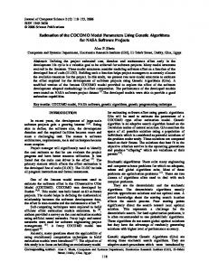
Predicted response of PVC at de/dt = 0.1 s -1 250
σT Total stress σA-α Intermolecular stress (α ) σA-α Intermolecular stress (β )
200
T0 = 250 K
σB Network stress (Langevin)
Fig. 1. Maxwell-Weichert element schematic of the MullikenBoyce constitutive model for polymers.
Stress [MPa]
T0 = 300 K T0 = 350 K
150
100
Table 1. Mulliken-Boyce parameters. Symbol σ
Parameter
50
Stress
ε, ε˙
Strain, strain rate
γ, γ˙
Shear strain, shear strain rate
τ, τ˙
Shear stress, shear stress rate
s
Athermal shear stress
θ
Temperature (absolute)
kB
Boltzmann’s constant
σ
Pressure
Cp
Heat capacity
ρ
Density
˙ θ) Eα (ε,
Young’s modulus (alpha)
˙ θ) Eβ (ε,
Young’s modulus (beta)
p (ε, ˙ θ) γ˙ α,0
Pre-exponential factor for shear strain rate (alpha)
p (ε, ˙ θ) γ˙ β,0
Pre-exponential factor for shear strain rate (beta)
∆Gα
Phase activation energy (alpha)
∆Gβ
Phase activation energy (beta)
αα
Pressure coefficient (alpha)
αβ
Pressure coefficient (beta)
hα
Softening slope (alpha)
hβ
Softening slope (beta)
s ss,α
Steady state preferred athermal shear stress (alpha)
s ss,β
Steady state preferred athermal shear stress (beta)
CR √ N
Rubbery modulus
0 0
0.1
0.2
0.3
0.4
0.5
0.6
0.7
0.8
0.9
1
Strain
Fig. 2. Simulated stress vs. strain relationship of PVC using Mulliken-Boyce model at three different temperatures.
rate-dependent parameters (currently being explored as an improvement to the solution). 2.2 Solution of ODE The nonlinear system of equations in Eq. (8) is solved using Matlab ODE solvers. The multistep ode113 function, based on the Adams-Bashforth-Moulton PECE solver [7], is used due to the computationally expensive nonlinear relationships. An example predicted response for PVC is shown in Figure 2 at a relatively low strain rate (ε˙ = 10 s−1 ) for three temperatures.
3 Bayesian inference of parameters
Limiting chain extensibility
It is important to note that the strain is carried forward as a time-dependent parameter in contrast with the standard practice of assuming constant strain rate. The remaining parameters are explained in Table 1. This addresses the practical issues of the early time response of polymers to incident stress waves where the system has not yet reached dynamic equilibrium and non-ideal experiments where the rate evolves continuously (i.e., never reaches equilibrium). Additionally, this approach enables the use of implicitly
Constitutive parameter estimation is an inverse problem wherein experimental data (observations) are used to infer the underlying parameter value(s) [8]. Bayesian statistics provide an intuitive, fundamental construct for the consideration of uncertainty in modeling, independent of its source (e.g., random experimental error vs. process-driven uncertainties). In this Bayesian framework, the conditional probability of the unknown parameters (x) based on the observed data (d) is the posterior probability distribution function (p) and is given for normally distributed data by � 1 1 p (x|d) = exp − [x − x0 ]T Γ−1 0 [x − x0 ] − ... N 2 � 1 (x)] [d − [d − m (x)]T Γ−1 − m (9) d 2 where m(x) is the model output based on the unknowns, x0 is the prior value for the unknown parameters, Γ0 is the
04041-p.2
DYMAT 2012 where ω is the angular frequency (in rad/s), d0 is the amplitude of the displacement, and lg is the specimen gage length. The corresponding time-temperature superposition for strain is typically included in the analysis using the WLF equation [14],
5000 Storage 4500
Loss × 10
4000
f = 100 Hz
Modulus [MPa]
3500 3000 2500
T =−
f = 1 Hz
f = 100 Hz
1000
f = 1 Hz 500 0 150
200
250
300 350 Temperature [K]
(12)
where T 0 and ω0 are reference quantities and C1 and C2 are constants. An alternative expression for he DMA shift [15, 16] is also considered, � � T = T 0 + A log ε˙ 0 − log ε˙ (13)
2000 1500
C2 ln (ω/ω0 ) − T0, [ln (ω/ω0 ) − C1 ]
400
450
500
Fig. 3. DMA storage and loss modulus data from PVC.
4.3 Phase transition statistical model
covariance matrix, Γd is the covariance matrix of the data, and N is a normalization constant. Maximizing Eq. (9) is accomplished using a maximum a posteriori (MAP) estimator. In the absence of available information, Bayes’ postulate states that a uniform prior probability should be assumed [9]. In the case of continuous variables, a uniform pdf over all x (called a diffuse, non-informative, or Dirichlet prior condition) is used, i.e., p(x) → ε x �
which parameterizes the shift using only two parameters, T 0 and the constant A.
(10)
where |x| < (2ε x )−1 and is ε−1 x sufficiently large to span the plausible range of x. Two different experimental data sets of PVC are analyzed, DMA and dynamic compression. The underlying parameters estimated are experiment-specific; these are reviewed in the next two sections.
4 DMA of PVC 4.1 Sample material and geometry PVC was chosen for study due to the availability of relevant data for comparison [10, 11]. Impact resistant PVC (Type II) was machined from extruded 25.4 mm diameter rods into samples that measured 60 mm long, 12.5 mm wide, and 3.2 mm thick. These samples were tested in a dual cantilever configuration in a TA Instruments Q800 [12, 13] at frequencies of 1, 10, and 100 Hz and a temperature range of −100◦ C to 190◦ C. The displacement was held constant at 15 µm for this analysis.
In the Mulliken-Boyce model, each of the two phases (α and β) are due to unique physical mechanisms. In Figure 3, the loss modulus show two distinct transitions that can be attributed to the phase: the α transition (i.e., the glass transition) occurs at T ≈ 350 K and the β transition occurs at T ≈ 200 K to 250 K. Since both the α and β transitions are spread over a finite temperature range, it is appropriate to consider each parameter as a statistical variable with underlying pdf’s. The form of these distributions for α and β processes are modeled differently. This is supported due to the statistical mechanics of the underlying transition [17], as discussed in the following sections. Additionally, the two phases’ properties, such as transition temperatures and activation energy, are assumed to be independent (not causally related). 4.3.1 Alpha phase The loss modulus of the glass transition (α phase) gives an indication of the irreversible conversion of mechanical energy into heat by the breaking of inter-chain bonds [17]. In a statistical interpretation, the loss modulus probability distribution pE �� α is the likelihood of the polymer bond being broken at a given temperature. The loss modulus of the α phase (E �� α ) is further assumed to be proportional to the temperature gradient of the storage modulus α phase (E � α ) i.e., (14) E �� α (T ) ∝ dE � α /dT The associated cumulative distribution function, χE �� α of the bond breaking distribution is given by � T � � pE �� α T � dT � (15) χE �� α (T ) = 0
4.2 Experimental DMA data and processing Typical DMA data for the PVC is shown in Figure 3 at the measured frequencies of 1, 10, and 100 Hz. The frequency is converted to strain rate (ε) ˙ equivalence relationship .[1],
which can be interpreted as the accumulated loss of polymer strength (i.e., storage modulus) due to the cumulative effect of bonds as the system heats through the glass transition. This is taken to be proportional to the storage modulus probability distribution, pE � α
ε˙ = 4ωd0 /lg ,
pEα� (T ) ∝ χE �� α (T )
(11) 04041-p.3
(16)
EPJ Web of Conferences
Mahieux [18] proposes a Weibull distribution [19] for the modulus of a polymer with respect to temperature, W(T ) due to the cascading interaction of ruptured bonds as it undergoes a glass transition. The probability distribution of the loss modulus, E� then assumes the form
Table 2. Estimation parameters and priors for DMA analysis.
pEα�� (T ) = W (T ; ∆Eα , T α , mα ) � �m −1 T �mα mα T α − e Tα , T ≥ 0, ∆E α T T (17) = α α 0, T