Protein Topology Classification
1
Protein Topology Classification using Two-Stage Support Vector Machines
1 2
Jayavardhana Gubbi1
Alistair Shilton1
[email protected]
[email protected]
Michael Parker2
M. Palaniswami1
[email protected]
[email protected]
Department of Electrical and Electronic Engineering, The University of Melbourne, Victoria - 3010, Australia St. Vincent’s Institute of Medical Research, 9 Princes Street, Fitzroy, Victoria 3065, Australia. Abstract
The determination of the first 3-D model of a protein from its sequence alone is a non-trivial problem. The first 3-D model is the key to the molecular replacement method of solving phase problem in x-ray crystallography. If the sequence identity is more than 30%, homology modelling can be used to determine the correct topology (as defined by CATH) or fold (as defined by SCOP). If the sequence identity is less than 25%, however, the task is very challenging. In this paper we address the topology classification of proteins with sequence identity of less than 25%. The input information to the system is amino acid sequence, the predicted secondary structure and the predicted real value relative solvent accessibility. A two stage support vector machine (SVM) approach is proposed for classifying the sequences to three different structural classes (α, β, α + β) in the first stage and 39 topologies in the second stage. The method is evaluated using a newly curated dataset from CATH with maximum pairwise sequence identity less than 25%. An impressive overall accuracy of 87.44% and 83.15% is reported for class and topology prediction, respectively. In the class prediction stage, a sensitivity of 0.77 and a specificity of 0.91 is obtained. Data file, SVM implementation (SVMHEAVY) and result files can be downloaded from http://www.ee.unimelb.edu.au/ISSNIP/downloads/.
Keywords: Protein Topology Classification, Kernel Methods, Support Vector Machines
1
Introduction
X-ray crystallography is one of the most popular experimental methods for determining the three dimensional structure of proteins. Indeed, more than 80% of the structures deposited into the protein data bank (PDB) [2] have been obtained using this method. One of the challenges when using this method is solving the phase problem [9]. A popular approach to this problem is the Molecular Replacement (MR) method [33], which is motivated by the observation that if the structures of two proteins are identical, then the diffraction patterns produced by them should be identical [9]. Based on this observation, the MR searches the PDB to find the protein therein which has the maximum sequence identity with the unknown protein. This known protein is called the first model. The phase of the first model is then combined with the intensity information of the unknown protein, and together these form a starting point for the calculation of the actual phase (and hence the three-dimensional structure) of the unknown protein. This latter process usually involves the determination of the positions of the model within the crystal cell using repeated rotation and translation functions [9, 33]. It is known [38] that if the protein sequence identity of the two proteins is greater than 35% then the proteins have similar structure. This knowledge is used in homology modeling to determine the
2
Gubbi et al.
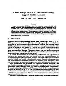
suitability of the first model. However this becomes challenging when the sequence identity is less than 35% (and even more so if the sequence identity is less than 25%) [38]. Three unique methods are available to define protein structure for experimentally determined models: FSSP (Fold classification based on Structure-Structure alignment of Proteins) [15], SCOP (Structural Classification of Proteins) [32] and CATH (Class, Architecture, Topology and Homology) [36]. FSSP uses Dali [16] for structure-structure alignment of proteins. SCOP divides the proteins into four hierarchical classes - Family, Superfamily, Fold and Class. FSSP and SCOP both use evolutionary relationships for classification. CATH is another type of hierarchical classification which uses the SSAP (Sequential Structure Alignment Program) [36] algorithm and is based on structural comparison. We choose to use CATH definitions and database for all the work reported in this paper as we found it to be more suitable for our future work. Fold recognition as defined by SCOP is nearest to topology as defined by CATH. Hence we review the literature for fold recognition followed by topology prediction methods. FORESST [7] uses secondary structure information and hidden markov models (HMM) for fold recognition. Ding and Dubchak [8, 10] combined support vector machines (SVMs) and neural networks for fold recognition. They tested their method on 27 SCOP folds with less than 25% sequence identity. Tan et. al. [42] used an ensemble machine learning approach for the same problem, and showed that their scheme was effective in scenarios where there are multi-class unbalanced datasets. Rangwala and Karypis [37] used SVMs with two novel kernels for fold recognition and remote homology detection. They used several profile based features in their work. Lund et. al. [28] proposed a method to construct the sequence profile for a sequence for which a ready template is not available. Fold and Function Assignment System (FFAS03) [18] tries to match profiles obtained from PSI-BLAST for fold recognition. 3DSHOTGUN [12, 13] is a meta-predictor which uses results from other major fold recognition schemes. It was rated in the top three servers in CAFASP3 experiments. SAM-T02 [24] uses HMM for protein structure prediction. This server has also proved to be very effective and is rated among the top servers. GenThreader [29] is another popular technique which uses feed forward neural network and predicted secondary structure for structure prediction. Relative to fold recognition, not much work has been done in the field of topology prediction. This is due to the fact that the classification method used by SCOP is based on evolutionary information, which is said to be more reliable then CATH. However, due to the convenience CATH provides for our future work, we have decided to use topology classification based on CATH. Early work by Francesco et. al. [6] used HMM for topology prediction from secondary structure, but can only be used on alpha class proteins. By contrast, in this paper we propose a method which first identifies the class (α, β, α + β) and then classifies between 39 topologies. A lot of work has been done toward predicting only the structural class (a nice review of which can be found in [5]). The most recent paper in structural class prediction was by Cao et. al. [4] and made use of the dataset by Zhou et. al. [47]. The maximum pairwise sequence identity of the Zhou datasets (taken from SCOP-1997) is not clearly indicated and hence it is difficult to compare this with our data. Our data is from a more recent version of CATH (2005) and is a hard dataset with maximum pairwise sequence identity less than 22% for 99.8% of the data. Furthermore, our work involves the more complex problem of topology prediction and hence it is different from class prediction methods. More recently Lo et. al. [27] used an SVM classifier for transmembrane helix and topology prediction. However the topology they define is entirely different to the CATH definitions that we use. In this paper, we propose a new method of predicting class and topology as defined by CATH [36]. We achieve this by using a two stage SVM. We develop a structure alignment kernel based on dynamic programming, predicted secondary structure and Chou-Fasman conformational parameters in the first stage. In the second stage, we use predicted solvent accessibility and evolutionary information in the form of position specific scoring matrix (PSSM) obtained from PSI-BLAST in an intuitive way and show that these simple features can produce some excellent results.
Protein Topology Classification Protein Sequence Sec Structure
......MEKFLVIAGPCAIESEELLLKVGEEIKRLSEKFKEVEFVFKSSFDKAN...... ......CCCEEEEEECCCCCCHHHHHHHHHHHHHHHHHCCCEEEEEEECCCCCC......
SVM Stage - 1
Alpha
1/2
SVM Stage - 2
3
2/3
1/3
Beta
Alpha+Beta
1/14
2/4
1/2
2/14
2/3
1/2
1/3
1/3 2/4
2/15
1/10
13/14 91 One vs. One classifiers
1/15
14/15 2/3
2/4
2/10
105 One vs. One classifiers
9/10 45 One vs. One classifiers
Decision by Voting
Figure 1: Proposed Classification Scheme
2
Material and Methods
We have constructed our dataset (which we call it GSPP742) using CATH version 2.6.0 (released in April 2005). This dataset can be downloaded from http://www.ee.unimelb.edu.au/ISSNIP/downloads/. To eliminate identical sequences, we have applied UniqueProt [31] with an HSSP-value of 5 to our dataset to eliminate identical sequences. We have retained only proteins with sequence length greater than 60 and resolution of at least 2 ˚ A in our dataset. After doing this, we are left with 946 proteins out of 10, 000+ which have pairwise identity of less than 30%. Finally, we have subjected all sequences to a pairwise global alignment algorithm to eliminate sequences with more than 25% identity. After this procedure, we are left with 742 sequences with a maximum pairwise sequence identity of less than 25%, of which less than 10 (0.01%) fall into the range 22%-25%. There are 164 proteins belonging to class α, 223 proteins belonging to class β and 355 proteins belonging to class α + β. Of the total 39 topologies, there are 14 topologies in class α, 10 topologies in class β and 15 topologies in class α + β. Our aim is to classify these proteins into three classes in first stage and 39 topologies in second stage. Our method makes use of two layers of support vector machines, as shown in figure 1. The system input is the protein sequence and its predicted secondary structure. At the first level, the protein sequences are classified into three classes as defined by CATH, namely α, β and α + β (which we will sometimes denote as γ). We do not make use of the fourth class, few secondary structures, as there are insufficient examples available for topologies in this class (with sequence identity less than 20%) to design a classifier. In the second stage, several binary classifiers are employed to differentiate 39 topologies (refer table 2) and the best match is selected using voting. In the absence of first stage of classification, to classify T topologies, 12 T (T − 1) binary classifiers are required. In our case, 741 classifiers would be required, which is infeasible. By the introduction of multi level classification, we are able to reduce the number of classifiers to 3 + 91 + 45 + 105 = 244 (3 classes in first stage followed by 14 α, 10 β and 15 γ topologies). We make use of predicted secondary structures [19] and predicted real value solvent accessibility [20] developed by our group. The prediction accuracy of the secondary structure method we use is in the range of 72% for unseen data. The cross-validation accuracy is 77%. To predict solvent accessibility, we have employed adaptive support vector regression [20]. The Mean Absolute Error (MAE) of solvent accessibility prediction using cross validation is approximately 0.12. The 8 to 3 state reduction method of secondary structure [23] used was H, G and I to H; E and B to E; and all others to C (where H stands for Alpha Helix, E for Beta Strand and C stands for Coil).
4
Gubbi et al.
Feature Extraction We extract Chou-Fasman conformational parameters separately for α class (class 1), β class (class 2) and α + β class (class 3). The Chou-Fasman parameter for a helix (H) in class 1 is given by P 1Hi = f 1Hi /hf 1H i where hf 1H i is the number of residues in the helix divided by the total number of residues; and the index i selects from the set of 20 amino acids residues. Similar conformational parameters for strand P 1Ei and coil P 1Ci were calculated for class 1. Hence P 1 is a 3 × 20 matrix with rows representing secondary structure states and columns representing amino acid residues. This notation is used in our new kernel development. The procedure is repeated for class 2 (P2) and class 3 (P3). This will be used for features for first stage of classification using the structure matching kernel described later. The folding free energy can be expressed as the summation of free energies due to intra molecular interaction and the interaction with the surrounding solvent molecules [35]. Most solvation models assume that the solvation energy of the solute is the sum of individual solvation energies of the residues. This would also give an indication about the position of the residue with respect to the core of protein which will enable the calculation of accessible surface area of a residue [17, 35]. These values (relative solvent accessibility - RSA) reflect the contribution of each side chain to the thermodynamic parameters of hydration which give an indication of hydrophobicity and hydrophilicity. We use predicted real values of RSA [20] as one of our features. We also extracted evolutionary information in the form of a position specific scoring matrix (PSSM) generated by PSI-BLAST [1] using the non-redundant (NR) database. The low complexity regions, coiled-coil regions and transmembrane helices were filtered with pfilt [22]. We chose an E-value of 0.0001 and 10 iterations for PSI-BLAST. The BLOSUM62 matrix was used for multiple sequence alignment. The RSA and evolutionary information extracted are used in the second level of classification. To ensure that the length of all feature vectors is constant irrespective of sequence length, we represent it in a unique way. The hydrophobicity scale so extracted is converted to a feature vector by taking the sum of the relative solvent accessibility (RSA) values for each amino acid. This contributes 20 dimensions to each feature vector. Similarly for evolutionary information, we calculate the sum of PSSM values for each amino acid for which the values are greater than 0, which contributes 20 more dimensions, giving a total of 40 dimensions for each feature vector. Intuitively, these give some indication of the contribution of each amino acid to the hydrophobicity scale and the evolutionary scale.
3
Support Vector Machines
Support Vector Machines introduced by Vapnik [45] has become one of the most popular tools in bioinformatics for supervised classification. These are binary classification algorithms based on structural risk minimization [46, 41, 3]. SVMs do this by implicitly mapping the training data into a (usually higher-dimensional) feature space. A hyperplane (decision surface) is then constructed in this feature space that bisects the two categories and maximises the margin of separation between itself and those points lying nearest to it (the support vectors). This decision surface can then be used as a basis for classifying vectors of unknown classification. The final decision function is given by [45, 39]: g (y) =
X
αi di K (xi , y) + b
(xi ,di )∈Θ
The function K(xi , xj ) = ϕ(xi )T ϕ(xj ) is called the kernel function, and plays a vital role in the SVM classifier. This is because the kernel function K completely hides the feature map ϕ :