Rapid, Stable Fluid Dynamics for Computer Graphics - CiteSeerX

~

ComputerGraphics,Volume24, Number4, August1990

Rapid, Stable Fluid Dynamics for Computer Graphics Michael Kass and Gavin Miller Advanced Technology Group A p p l e C o m p u t e r , Inc. 20705 V a l l e y G r e e n D r i v e C u p e r t i n o , C A 95014

ABSTRACT

INTRODUCTION

We present a new method for animating water based on a simple, rapid and stable solution of a set of partial differential equations resulting from an approximation to the shallow water equations. The approximation gives rise to a version of the wave equation on a height-field where the wave velocity is proportional to the square root of the depth of the water. The resulting wave equation is then solved with an altematingdirection implicit method on a uniform finite-difference grid. The computational work required for an iteration consists mainly of solving a simple tridiagonal linear system for each row and column of the height field. A single iteration per frame suffices in most cases for convincing animation. Like previous computer-graphics models of wave motion, the new method can generate the effects of wave refraction with depth. Unlike previous models, it also handles wave reflections, net transport of water and boundary conditions with changing topology. As a consequence, the model is suitable for animating phenomena such as flowing rivers, raindrops hitting surfaces and waves in a fish tank as well as the classic phenomenon of waves lapping on a beach. The height-field representation prevents it from easily simulating phenomena such as breaking waves, except perhaps in combination with particle-based fluid models. The water is rendered using a form of caustic shading which simulates the refraction of illuminating rays at the water surface. A wemess map is also used to compute the wetting and drying of sand as the water passes over it.

The problem of realistically modeling scenes containing water has captured the attention of a number of computergraphics researchers in recent years[l; 2; 3; 4; 51, The omnipresence of water as well as the complexities and subtleties of its motion have made it an attractive subject of study. Yet existing computer-graphics models of water motion adequately cover only a very small range of interesting water phenomena. Among other effects, they fail to account for wave reflections, net transport of water and boundary conditions with changing topology. A computationally inexpensive method of simulating these phenomena will be presented here. Based on solving a partial-differential equation on the surface of a height-field, the method is easy to implement and very stable. The approximations involved may not be suitable for high-precision engineering applications, but they produce pleasing animation with little effort. Many popular methods for modeling water surfaces work well for producing still images, but are unsuitable for animation because they do not include realistic models for the evolution of the surface over time. Examples of these techniques include stochastic subdivision [6] and Fourier synthesis [5]. Other techniques work well only in large bodies of water away from boundaries [7; 1; 8]. Recently, the realism of water modeling in computer graphics was substantially improved by three papers [2; 3; 4-] that took into account refraction due to changing wave velocity with depth. In each case, specialized methods based on tracking individual waves or wave-trains were used to avoid the need to directly solve a differential equation. These papers deal adequately with waves hitting a beach, but they leave a wide range of water phenomena unexplored. None of the papers includes simulations of reflected waves. In addition, the underlying model in each case is that particles of water move in circular or ellipsoidal orbits around their initial positions, so there can be no net transport or flow. Finally, none of the papers considers situations in which the boundary conditions change through time altering the topology of the water -- for example a wave pushing water up over an obstacle and down the other side to create a puddle. It appears to be very difficult to deal with these phenomena efficiently by tracing waves. Two alternatives to tracing the propagation of waves or wave-trains exist. One is to simulate the fluid by the interaction of a large number of particles [9; 101, and the other is to directly solve a partial differential equation describing the fluid dynamics [11; 12; 13]. Both have been used by hydrodynamicists to create iterative simulations of fluid flow. The problem is that a truly accurate simulation of fluid mechanics usually requires computing the motion throughout a volume. This means that the amount of computation per iteration grows at least as the cube of the resolution. If there are linear

CR Categories a n d Subject Descriptors: 1.3.7: [Computer Graphics]: Graphics and Realism: Animation; G.1.8: [Mathematics of Computing]: Partial Differential Equations; 1.6.3 [Simulation and Modeling]: Applications.

Additional Keywords and Phrases:

Wave equation, fluid dynamics, flow, finite-difference, height-field, caustic.

Permission to copy without fee all or part of this material is granted provided that the copies are not made or distributed for direct commercial advantage, the ACM copyright notice and the title of the publication and its date appear, and notice is given that copying is by permission of the Association for Computing Machinery. To copy otherwise, or to republish, requires a fee and/or specific permission.

©1990

ACM-0-89791-34.4-2/90/008/0049

$00.75

49

SIGGRAPH '90, Dallas, August 6-10, 1990

h0

h1

h2

ha

...

hn.3

ha.2

hn.1

b0

bI

b2

b3

• . .

b~.3

b._2

b~.l

U0

U1

Un_3

Un.2

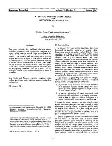
Fig. 1: Discretetwo-dimensionalheight-fieldrepresentationof the water surface h, the groundbottom b, and the horizontalwater velocity u.

sumption will not introduce error. The second assumption is that the vertical component of the velocity of the water particles can be ignored. Once again, the limitations of this assumption are fairly clear. If a disturbance creates very steep waves on the water surface, the model will cease to be accurate. The third assumption is that the horizontal component of the velocity of the water in a vertical column is approximately constant. If there is turbulent flow or unusually high friction on the bottom, this assumption will break down. Nonetheless, the experience of hydrodYnamicists suggests that this is a very useful approximation to phenomena ranging from the effect of a single rain drop to the refraction of waves in a sea port. For simplicity, we begin with a height-field curve in two dimensions. Later, the same techniques will be extended to a height-field surface in three dimensions. Let z = h(x) be the height of the water surface and let z = b(x) be the height of the ground, tf d(x)=h(x)-b(x) is the water depth and u(x) is the horizontal velocity of a vertical column of water, the shallow water equations that follow from the above assumptions[ 16; 17] can be written as follows:

-ON - + u NoN+ a g ,gd

systems to be solved at every iteration, the computational cost can grow even faster. In addition, the number of iterations required may grow as the resolution is increased. As a consequence, accurate simulation of fluid mechanics is typically reserved for vectorized supercomputers or very highly parallel machines. For the purposes of animation, accuracy is much less important than stability and speed. An animator using techniques of physical simulation will typically have to experiment with a number of different conditions of a simulation before achieving satisfying motion. If the experiments take too much time or if the numerical methods become unstable, the process can become excruciating. Here, we examine the differential equation approach with the goal of constructing the fastest stable simulation which yields a wide range of convincing motion. We begin by considering a very simplified subset of water flow where the water surface can be represented as a height field and the motion is uniform through a vertical column. This subset of water flow is representative of a variety of non-turbulent shallow-water phenomena. Under these conditions, we can approximate the equations of motion of the water in terms of a grid of points on a height-field. The amount of computation can then be proportional to the number of samples on the surface of the water which varies as the square of the resolution instead of the cube. Integration of the partial-differential equations is done with an alternating-direction implicit technique [14]. The result is a very stable integration scheme which is also very fast. Stability derives from the use of an implicit integration scheme; speed derives from the tridiagonal structure of the required linear systems which are solvable in linear time. Because of the stability, the time-step of the solution can be made equal to the frame time of the animation in most cases.

SHALLOW WATER EQUATIONS In lieu of simulating the full Navier-Stokes equations of fluid flow, we begin with a vastly simplified set of equations which has been widely used for shallow water [15; 16; 17]. The simplification arises from three approximations. The first approximation is that the water surface is a height field. This, of course, has some obvious limitations. The water cannot splash and waves cannot break. However, so long as the forces on the water are sufficiently gentle, the height-field as-

50

Oh

at

0

-~- + ~

(ud) = 0

=0

(eq. 1)

(eq. 2)

where g is the gravitational acceleration. Eq. 1 expresses Newton's law F=ma while eq. 2 expresses the constraint of volume conservation. Note that even with the above three simplifying assumptions, the resulting differential equations are non-linear. A further simplification which is often used is to ignore the second term in eq. 1 and linearize around a constant value of h. This will be reasonable if the fluid velocity is small and the depth is slowly varying. The resulting equations are then:

oh

--+g~=0 at

(eq. 3)

Oh ON -5-+d-g = 0

(eq. 4)

If we differentiate eq. 3 with respect to x, then differentiate eq. 4 with respect to t and finally substitute for the cross-derivatives, we end up with d 2h at 2

-

gd

d 2h 0x 2

(eq. 5)

which is the one-dimensional wave equation with wave velocity ~ . While this degree of simplification is suspect for many engineering purposes, our experience suggests that the resulting equations are quite adequate for a wide range of animation applications.

DISCRETIZATION In order to solve eq. 5, we need to construct a discrete representation of the continuous partial-differential equation. There are two established techniques for doing so. The first is the finite-difference technique where the continuous functions are represented by a collection of samples. The second is the finite-element technique where the continuous functions are represented as the sum of a collection of continuous basis functions. Here, the finite-difference technique works particularly well because of the simple height-field representation. The resulting algorithm is very easy to implement and the

~

linear systems involved are tridiagonal. Figure 1 shows the discrete representation of the heightfield in two dimensions. Note that the samples for u lie halfway in between the samples of h. After experimenting with a number of finite-difference approximations to equations 3 and 4, the most stable version we have found is Ohi

( di_l + d i

-;:

t. 3m