Reference Guide on Multiple Regression

Reference Guide on Multiple Regression

Daniel L. Rubinfeld

Daniel L. Rubinfeld, J.D., Ph.D., is Professor of Law and Professor of Economics, University of California, Berkeley.

Contents

I. Introduction 419 II. Research Design: Model Specification 423 A. What Is the Specific Question That Is Under Investigation by the Expert? 423 B. What Model Should Be Used to Evaluate the Question at Issue? 423 1. Choosing the dependent variable 424 2. Choosing the explanatory variable that is relevant to the issues in the case 424 3. Choosing the additional explanatory variables 424 4. Choosing the functional form of the multiple regression model 426 5. Choosing multiple regression as a method of analysis 427 III. Interpreting Regression Results 429 A. What Is the Practical as Opposed to the Statistical Significance of Regression Results? 429 1. When should statistical tests of significance be used? 430 2. What is the appropriate level of statistical significance? 431 3. Should statistical tests be one-tailed or two-tailed? 431 B. Are the Regression Results Robust—Sensitive to Changes in Assumptions and Procedures? 432 1. What evidence exists that the explanatory variable causes changes in the dependent variable? 432 2. To what extent are the explanatory variables correlated with each other? 434 3. To what extent are individual errors in the regression model independent? 435 4. To what extent are the regression results sensitive to individual data points? 436 5. To what extent are the data subject to measurement error? 437 IV. The Expert 439 V. Presentation of Statistical Evidence 441

417

A. What Disagreements Exist Regarding Data on Which the Analysis Is Based? 441 B. What Database Information and Analytical Procedures Will Aid in Resolving Disputes over Statistical Studies? 442 Appendix: The Basics of Multiple Regression 445 Glossary of Terms 463 References on Multiple Regression 469

418

Reference Manual on Scientific Evidence

I. Introduction

Multiple regression analysis is a statistical tool for understanding the relationship between two or more variables.1 Multiple regression involves a variable to be explained—called the dependent variable—and additional explanatory variables that are thought to produce or be associated with changes in the dependent variable. 2 For example, a multiple regression analysis might estimate the effect of the number of years of work on salary. Salary would be the dependent variable to be explained; years of experience would be the explanatory variable. Multiple regression analysis is sometimes well suited to the analysis of data about competing theories in which there are several possible explanations for the relationship among a number of explanatory variables. 3 Multiple regression typically uses a single dependent variable and several explanatory variables to assess the statistical data pertinent to these theories. In a case alleging sex discrimination in salaries, for example, a multiple regression analysis would examine not only sex, but also other explanatory variables of interest, such as education and experience. 4 The employer–defendant might use multiple regression to argue that salary is a function of the employee’s

1. A variable is anything that can take on two or more values (e.g., the daily temperature in Chicago). 2. Explanatory variables in the context of a statistical study are also called independent variables. See David H. Kaye & David A. Freedman, Reference Guide on Statistics § II.C.1, in this manual. Kaye and Freedman also offer a brief discussion of regression analysis. Id . § III.F.3. 3. Multiple regression is one type of statistical analysis involving several variables. Other types include matching analysis, stratification, analysis of variance, probit analysis, logit analysis, discriminant analysis, and factor analysis. 4. Thus, in Ottaviani v. State Univ. of N.Y., 875 F.2d 365, 367 (2d Cir. 1989), cert. denied, 493 U.S. 1021 (1990), the court stated: In disparate treatment cases involving claims of gender discrimination, plaintiffs typically use multiple regression analysis to isolate the influence of gender on employment deci sions relating to a particular job or job benefit, such as salary. The first step in such a re gression analysis is to specify all of the possible “legitimate” (i.e., nondiscriminatory) fac tors that are likely to significantly affect the dependent variable and which could account for disparities in the treatment of male and female employees. By identifying those legit imate criteria that affect the decision making process, individual plaintiffs can make pre dictions about what job or job benefits similarly situated employees should ideally re ceive, and then can measure the difference between the predicted treatment and the ac tual treatment of those employees. If there is a disparity between the predicted and ac tual outcomes for female employees, plaintiffs in a disparate treatment case can argue that the net “residual” difference represents the unlawful effect of discriminatory animus on the allocation of jobs or job benefits. (citations omitted)

419

education and experience, and the employee–plaintiff might argue that salary is also a function of the individual’s sex. Multiple regression also may be useful (1) in determining whether or not a particular effect is present; (2) in measuring the magnitude of a particular effect; and (3) in forecasting what a particular effect would be, but for an intervening event. In a patent infringement case, for example, a multiple regression analysis could be used to determine (1) whether the behavior of the alleged infringer affected the price of the patented product; (2) the size of the effect; and (3) what the price of the product would have been had the alleged infringement not occurred. Over the past several decades the use of regression analysis in court has grown widely. 5 Although multiple regression analysis has been used most frequently in cases of sex and race discrimination 6 and antitrust violation, 7 other applications have ranged across a variety of cases, including those involving census undercounts,8 voting rights, 9 the study of the deterrent effect of the death penalty, 10 and intellectual property. 11 5. There were only 2 WESTLAW references to multiple regression in federal cases between 1960 and 1969, 26 references between 1970 and 1979, 204 references between 1980 and 1989, and 73 references since 1990. 6. Recent discrimination cases using multiple regression analysis include King v. General Elec. Co., 960 F.2d 617 (7th Cir. 1992), and Tennes v. Massachusetts Dep’t of Revenue, No. 88-C3304, 1989 WL 157477 (N.D. Ill. Dec. 20, 1989) (age discrimination); EEOC v. General Tel. Co. of N.W., 885 F.2d 575 (9th Cir. 1989), cert. denied, 498 U.S. 950 (1990), Churchill v. International Business Machs., Inc., 759 F. Supp. 1089 (D.N.J. 1991), and Denny v. Westfield State College, 880 F.2d 1465 (1st Cir. 1989) (sex discrimination); Black Law Enforcement Officers Ass’n v. City of Akron, 920 F.2d 932 (6th Cir. 1990), Bazemore v. Friday, 848 F.2d 476 (4th Cir. 1988), Bridgeport Guardians, Inc. v. City of Bridgeport, 735 F. Supp. 1126 (D. Conn. 1990), aff’d , 933 F.2d 1140 (2d Cir.), cert. denied, 112 S. Ct. 337 (1991), and Dicker v. Allstate Life Ins. Co., No. 89C4982, 1193 WL 62385 (N.D. Ill. Mar. 5, 1993) (race discrimination). 7. Recent antitrust cases using multiple regression analysis include In re Chicken Antitrust Litig., 560 F. Supp. 963, 993 (N.D. Ga. 1980); and United States v. Brown Univ., 805 F. Supp. 288 (E.D. Pa. 1992), rev’d , 5 F.3d 658 (3d Cir. 1993) (price fixing of college scholarships). 8. See, e.g., Carey v. Klutznick, 508 F. Supp. 420, 432–33 (S.D.N.Y. 1980) (use of reasonable and scientif ically valid statistical survey or sampling procedures to adjust census figures for the differential undercount is constitutionally permissible), stay granted, 449 U.S. 1068 (1980), rev’d on other grounds , 653 F.2d 732 (2d Cir. 1981), cert. denied, 455 U.S. 999 (1982); Young v. Klutznick, 497 F. Supp. 1318, 1331 (E.D. Mich. 1980), rev’d on other grounds, 652 F.2d 617 (6th Cir. 1981), cert. denied, 455 U.S. 939 (1982); Cuomo v. Baldrige, 674 F. Supp. 1089 (S.D.N.Y. 1987). 9. Multiple regression analysis was used in suits charging that at-large area-wide voting was instituted to neutralize black voting strength. Multiple regression demonstrated that the race of the candidates and that of the electorate was a determinant of voting. See Kirksey v. City of Jackson, 461 F. Supp. 1282, 1289 (S.D. Miss. 1978), aff’d , 663 F.2d 659 (5th Cir. 1981); Brown v. Moore, 428 F. Supp. 1123, 1128–29 (S.D. Ala. 1976), aff’d without op. , 575 F.2d 298 (5th Cir. 1978), vacated sub nom . Williams v. Brown, 446 U.S. 236 (1980); Bolden v. City of Mobile, 423 F. Supp. 384, 388 (S.D. Ala. 1976), aff’d , 571 F.2d 238 (5th Cir. 1978), stay de nied , 436 U.S. 902 (1978), and rev’d , 446 U.S. 55 (1980); Jeffers v. Clinton, 730 F. Supp. 196, 208–09 (E.D. Ark. 1989), aff’d , 498 U.S. 1019 (1991); and League of United Latin Am. Citizens, Council No. 4434 v. Clements, 986 F.2d 728, 774–87 (5th Cir.), reh’g en banc , 999 F.2d 831 (5th Cir. 1993), cert. denied, 114 S. Ct. 878 (1994). For a recent update on statistical issues involving voting rights cases, see Daniel L. Rubinfeld, Statistical and Demographic Issues Underlying Voting Rights Cases, 15 Evaluation Rev. 659 (1991), and the as sociated articles within Vol. 15 (a special symposium issue devoted to statistical and demographic issues under lying voting rights cases). 10. See, e.g ., Gregg v. Georgia, 428 U.S. 153, 184–86 (1976). For a critique of the validity of the deter rence analysis, see National Research Council, Deterrence and Incapacitation: Estimating the Effects of Criminal Sanctions on Crime Rates (Alfred Blumstein et al. eds., 1978). Multiple regression methods have been used to

420


Multiple regression analysis can be a source of valuable scientific testimony in litigation. However, when inappropriately used, regression analysis can confuse important issues while having little, if any, probative value. In EEOC v. Sears, Roebuck & Co ., in which Sears was charged with discrimination against women in hiring practices, the Seventh Circuit acknowledged that “[m]ultiple regression analyses, designed to determine the effect of several independent variables on a dependent variable, which in this case is hiring, are an accepted and common method of proving disparate treatment claims.”12 However, the court affirmed the district court’s findings that the “E.E.O.C’s regression analyses did not ‘accurately reflect Sears’ complex, nondiscriminatory decision-making processes’” and that “‘E.E.O.C.’s statistical analyses [were] so flawed that they lack[ed] any persuasive value.’” 13 Serious questions also have been raised about the use of multiple regression analysis in census undercount cases and in death penalty cases.14 Moreover, in interpreting the results of a multiple regression analysis, it is important to distinguish between correlation and causality. Two variables are correlated when the events associated with the variables occur more frequently together than one would expect by chance. For example, if higher salaries are associated with a greater number of years of work experience, and lower salaries are associated with fewer years of experience, there is a positive correlation between the two variables. However, if higher salaries are associated with less experience, and lower salaries are associated with more experience, there is a negative correlation between the two variables. A correlation between two variables does not imply that one event causes the second to occur. Therefore, in making causal inferences, it is important to avoid spurious correlation .15 Spurious correlation arises when two variables are closely related but bear no causal relationship because they are both caused by a third, unexamined variable. For example, there might be a negative correlation between the age of certain skilled employees of a computer company and their salaries. One should not evaluate whether the death penalty was applied discriminately on the basis of race. See McClesky v. Kemp, 481 U.S. 279, 292–94 (1987). 11. See Polaroid Corp. v. Eastman Kodak Co., No. 76-1634-MA, 1990 WL 324105, at *29, 62–63 (D. Mass. Oct. 12, 1990) (damages due to patent infringement), amended by No. 76-1634-MA, 1991 WL 4087 (D. Mass. Jan. 11, 1991); and Estate of Vane v. The Fair, Inc., 849 F.2d 186, 188 (5th Cir. 1988), cert. denied, 488 U.S. 1008 (1989) (lost profits due to copyright infringement). 12. 839 F.2d 302, 324 n.22 (7th Cir. 1988). 13. Id. at 348, 351 (quoting EEOC v. Sears, Roebuck & Co., 628 F. Supp. 1264, 1342, 1352 (N.D. Ill. 1986)). The district court comments specifically on the “severe limits of regression analysis in evaluating com plex decision-making processes.” 628 F. Supp. at 1350. 14. With respect to the census, see Stephen E. Fienberg, The New York City Census Adjustment Trial: Witness for the Plaintiffs, 34 Jurimetrics J. 65 (1993); John E. Rolph, The Census Adjustment Trial: Reflections of a Witness for the Plaintiffs, 34 Jurimetrics J. 85 (1993); David A. Freedman, Adjusting the Census of 1990, 34 Jurimetrics J. 107 (1993). Concerning the death penalty, see Richard Lempert, Capital Punishment in the ‘80’s: Reflections on the Symposium, 74 J. Crim. L. & Criminology 1101 (1983). 15. See Linda A. Bailey et al., Reference Guide on Epidemiology § IV.A (Confounding Variables), and David H. Kaye & David A. Freedman, Reference Guide on Statistics §§ II.C.2, III.F.2.c, in this manual.

Multiple Regression

421

conclude from this correlation that the employer has necessarily discriminated against the employees on the basis of their age. A third, unexamined variable— the level of the employees’ technological skills—could explain differences in productivity and, consequently, differences in salary. Or, consider a patent infringement damage case in which increased sales of an allegedly infringing product are associated with a lower price of the patented product. This correlation would be spurious if the two products have their own noncompetitive market niches and the lower price is due to a decline in the production costs of the patented product. Causality cannot be inferred by data analysis alone—rather, one must infer that a causal relationship exists on the basis of an underlying causal theory that explains the relationship between the two variables. Even when an appropriate theory has been identified, causality can never be inferred directly—one must also look for empirical evidence that there is a causal relationship. Conversely, the presence of a non-zero correlation between two variables does not guarantee the existence of a relationship; it could be that the model does not reflect the correct interplay among the explanatory variables. In fact, the absence of correlation does not guarantee that a causal relationship does not exist. Rather, lack of correlation could occur if (1) there are insufficient data; (2) the data are measured inaccurately; (3) the data do not allow multiple causal relationships to be sorted out; or (4) the model is specified wrongly. There is a tension between any attempt to reach conclusions with near certainty and the inherently probabilistic nature of multiple regression analysis. In general, statistical analysis involves the formal expression of uncertainty in terms of probabilities. The reality that statistical analysis generates probabilities that there are relationships should not be seen in itself as an argument against the use of statistical evidence. The only alternative might be to use less reliable anecdotal evidence. This reference guide addresses a number of procedural and methodological issues that are relevant in considering the admissibility of, and weight to be accorded to, the findings of multiple regression analyses. It also suggests some standards of reporting and analysis that an expert presenting multiple regression analyses might be expected to meet. Section II discusses research design—how the multiple regression framework can be used to sort out alternative theories about a case. Section III concentrates on the interpretation of the multiple regression results, from both a statistical and a practical point of view. Section IV briefly discusses the qualifications of experts. In section V the emphasis turns to procedural aspects associated with the use of the data underlying regression analyses. Finally, the Appendix delves into the multiple regression framework in further detail; it also contains a number of specific examples that illustrate the application of the technique. A list of statistical references and a glossary are also included.

422


II. Research Design: Model Specification

Multiple regression allows the expert to choose among alternative theories or hypotheses and assists the expert in sorting out correlations between variables that are plainly spurious from those that reflect valid relationships.

A. What Is the Specific Question That Is Under Investigation by the Expert? Research begins with a clear formulation of a research question. The data to be collected and analyzed must relate directly to the immediate issue; otherwise, appropriate inferences cannot be drawn from the statistical analysis. For example, if the question at issue in a patent damage case is what price the plaintiff’s product would have been but for the sale of the defendant’s infringing product, sufficient data must be available to allow the expert to account statistically for the important factors that determine the price of the product.

B. What Model Should Be Used to Evaluate the Question at Issue? Model specification involves several steps, each of which is fundamental to the success of the research effort. Ideally, a multiple regression analysis builds on a theory that describes the variables to be included in the study. For example, the theory of labor markets might lead one to expect salaries in an industry to be related to workers’ experience and the productivity of workers’ jobs. A belief in discrimination would lead one to add a variable or variables reflecting discrimination to the model. Models are often characterized in terms of parameters —numerical characteristics of the model. In the labor market example, one parameter might reflect the increase in salary associated with each additional year of job experience. Multiple regression uses a sample , or a selection of data, from the population , or all the units of interest, to obtain estimates of the values of the parameters of the model—an estimate associated with a particular explanatory variable is a regres sion coefficient . Failure to develop the proper theory, failure to choose the appropriate variables, and failure to choose the correct form of the model can bias substantially

423

the statistical results, that is, create a systematic tendency for an estimate of a model parameter to be too high or too low. 1. Choosing the dependent variable The variable to be explained should be the appropriate variable for analyzing the question at issue. 16 Suppose, for example, that pay discrimination among hourly workers is a concern. One choice for the dependent variable is the hourly wage rate of the employees; another choice is the annual salary. The distinction is important, because annual salary differences may be due in part to differences in hours worked. If the number of hours worked is the product of worker preferences and not discrimination, the hourly wage is a good choice. If the number of hours is related to the alleged discrimination, annual salary is the more appropriate dependent variable to choose. 17 2. Choosing the explanatory variable that is relevant to the issues in the case The explanatory variable that allows the evaluation of alternative hypotheses must be chosen appropriately. Thus, in a discrimination case, the variable of in terest may be the race or sex of the individual. In an antitrust case, it may be a variable that takes on the value 1 to reflect the presence of the alleged anticompetitive behavior and a value 0 otherwise. 18 3. Choosing the additional explanatory variables An attempt should be made to identify the additional known or hypothesized explanatory variables, some of which are measurable and may support alternative substantive hypotheses that can be accounted for by the regression analysis. Thus, in a discrimination case, a measure of the skill level of the work may provide an alternative explanation—lower salaries were the result of inadequate skills. 19 16. In multiple regression analysis, the dependent variable is usually a continuous variable that takes on a range of numerical values. When the dependent variable is categorical, taking only two or three values, modi fied forms of multiple regression, such as probit or logit analysis, are appropriate. For an example of the use of the latter, see EEOC v. Sears, Roebuck & Co., 839 F.2d 302, 325 (7th Cir. 1988) (EEOC used weighted logit analysis to measure the impact of variables, such as age, education, job type experience, and product line expe rience, on the female percentage of commission hires). See also David H. Kaye & David A. Freedman, Reference Guide on Statistics § II.C.1, in this manual. 17. In job systems in which annual salaries are tied to grade or step levels, the annual salary corresponding to the job position could be more appropriate. 18. Explanatory variables may vary by type, which will affect the interpretation of the regression results. Thus, some variables may be continuous, taking on a wide range of values, while others may be categorical, taking on only two or three values. 19. In Ottaviani v. State Univ. of N.Y., 679 F. Supp. 288, 306–08 (S.D.N.Y. 1988), aff’d , 875 F.2d 365 (2d Cir. 1989), cert. denied , 493 U.S. 1021 (1990), the court ruled (in the liability phase of the trial) that the uni versity showed there was no discrimination in either placement into initial rank or promotions between ranks, so rank was a proper variable in multiple regression analysis to determine whether women faculty members were treated differently from men. However, in Trout v. Garrett, 780 F. Supp. 1396, 1414 (D.D.C. 1991), the court ruled (in the damage phase of the trial) that the extent of civilian employees’ prehire work experience was not an appropriate vari able

424


Not all possible variables that may influence the dependent variable can be included if the analysis is to be successful—some cannot be measured, and others may make little difference. 20 If a preliminary analysis shows the unexplained portion of the multiple regression to be unacceptably high, the expert may seek to discover whether some previously undetected variable is missing from the analysis. 21 Failure to include a major explanatory variable that is correlated with the variable of interest in a regression model may cause an included variable to be credited with an effect that actually is caused by the excluded variable. 22 In general, omitted variables that are correlated with the dependent variable reduce the probative value of the regression analysis. 23 This may lead to inferences made from regression analyses that do not assist the trier of fact. 24 Omitting variables that are not correlated with the variable of interest is, in general, less of a concern, since the parameter that measures the effect of the variable of interest on the dependent variable is estimated without bias. Suppose, for example, that the effect of a policy introduced by the courts to encourage child support has been tested by randomly choosing some cases to be handled according to current court policies and other cases to be handled according to a new, more stringent policy. The effect of the new policy might be measured by a multiple regression using payment success as the dependent variable and a 0 or 1 explanatory variable (1 if the new program was applied; 0 if it was not). Failure in a regression analysis to compute back pay in employment discrimination. According to the court, in cluding the prehire level would have resulted in a finding of no sex discrimination, despite a contrary conclu sion in the liability phase of the action. Id. See also Stuart v. Roache, 951 F.2d 446 (1st Cir. 1991) (allowing only three years of seniority to be considered due to prior discrimination), cert. denied, 112 S. Ct. 1948 (1992). 20. The summary effect of the excluded variables shows up as a random error term in the regression model, as does any modeling error. See infra the Appendix for details. 21. A very low R-square (R 2 ) is one indication of an unexplained portion of the multiple regression model that is unacceptably high. For reasons discussed in the Appendix, however, a low R 2 does not necessarily imply a poor model (and vice versa). 22. Technically, the omission of explanatory variables which are correlated with the variable of interest can cause biased estimates of regression parameters. 23. The effect tends to be important, the stronger the relationship between the omitted variable and the dependent variable, and the stronger the correlation between the omitted variable and the explanatory vari ables of interest. 24. See Bazemore v. Friday, 751 F.2d 662, 671–72 (4th Cir. 1984) (upholding the district court’s refusal to accept a multiple regression analysis as proof of discrimination by a preponderance of the evidence, the court of appeals stated that, although the regression used four variable factors, consisting of race, education, tenure, and job title, the failure to use other factors, including pay increases which varied by county, precluded their introduction into evidence), aff’d in part , vacated in part , 478 U.S. 385 (1986). Note, however, that in Sobel v. Yeshiva Univ., 839 F.2d 18, 33, 34 (2d Cir. 1988), cert. denied , 490 U.S. 1105 (1989), the court made clear that “a [Title VII] defendant challenging the validity of a multiple regres sion analysis [has] to make a showing that the factors it contends ought to have been included would weaken the showing of salary disparity made by the analysis,” by making a specific attack and “a showing of relevance for each particular variable it contends . . . ought to [be] includ[ed]” in the analysis, rather than by simply at tacking the results of the plaintiffs’ proof as inadequate for lack of a given variable. Also, in Bazemore v. Friday, the Court, declaring that the Fourth Circuit’s view of the evidentiary value of the regression analyses was plainly incorrect, stated that “[n]ormally, failure to include variables will affect the analysis’ probativeness, not its admissibility. Importantly, it is clear that a regression analysis that includes less than ‘all measurable variables’ may serve to prove a plaintiff’s case.” 478 U.S. 385, 400 (1986) (footnote omit ted).

Multiple Regression

425

to include an explanatory variable that reflected the age of the husbands involved in the program would not affect the court’s evaluation of the new policy, since men of any given age are as likely to be affected by the old as the new policy. Choosing the court’s policy by chance has ensured that the omitted age variable is not correlated with the policy variable. Bias caused by the omission of important variables that are related to the included variables of interest can be a serious problem. 25 Nevertheless, it is possible to account for bias qualitatively if the expert has knowledge (even if not quantifiable) about the relationship between the omitted variable and the explanatory variable. Suppose, for example, that the plaintiff’s expert in a sex discrimination pay case is unable to obtain quantifiable data that reflect the skills necessary for a job, and that, on average, women are more skillful than men. Suppose also that a regression of the wage rate of employees (the dependent variable) on years of experience and a variable reflecting the sex of each employee (the explanatory variable) suggests that men are paid substantially more than women with the same experience. Because differences in skill levels have not been taken into account, the expert may conclude reasonably that the wage difference measured by the regression is a conservative estimate of the true discriminatory wage difference. The precision of the measure of the effect of a variable of interest on the dependent variable is also important. 26 In general, the more complete the explained relationship between the included explanatory variables and the dependent variable, the more precise the results. Note, however, that the inclusion of explanatory variables that are irrelevant (i.e., that are not correlated with the dependent variable) reduces the precision of the regression results. This can be a source of concern when the sample size is small, but it is not likely to be of great consequence when the sample size is large. 4. Choosing the functional form of the multiple regression model Choosing the proper set of variables to be included in the multiple regression model does not complete the modeling exercise. The expert must also choose the proper form of the regression model. The most frequently selected form is the linear regression model (described in the Appendix). In this model the magnitude of the change in the dependent variable associated with the change in any of the explanatory variables is the same no matter what the level of that explanatory variable. For example, one additional year of experience might add $5,000 to salary, irrespective of the previous experience of the employee.

25. See also Linda A. Bailey et al., Reference Guide on Epidemiology § IV.A, and David H. Kaye & David A. Freedman, Reference Guide on Statistics § II.C.2, in this manual. 26. A more precise estimate of a parameter is an estimate with a smaller standard error. See infra the Appendix for details.

426


In some instances, however, there may be reason to believe that changes in explanatory variables will have differential effects on the dependent variable as the values of the explanatory variables change. In this case, the expert should consider the use of a nonlinear model . Failure to account for nonlinearities can lead to either overstatement or understatement of the effect of a change in the value of an explanatory variable on the dependent variable. One particular type of nonlinearity involves the interaction among several variables. An interaction variable is the product of two other variables that are included in the multiple regression model. The interaction variable allows the expert to take into account the possibility that the effect of a change in one variable on the dependent variable may change as the level of another explanatory variable changes. For example, in a salary discrimination case, the inclusion of a term that interacts a variable measuring experience with a variable representing the sex of the employee (1 if a female employee, 0 if a male employee) allows the expert to test whether the sex differential varies with the level of experience. A significant negative estimate of the parameter associated with the sex variable suggests that inexperienced women are discriminated against, while a significant negative estimate of the interaction parameter suggests that the extent of discrimination increases with experience. 27 Note that insignificant coefficients in a model with interactions may suggest a lack of discrimination, while a model without interactions may suggest the contrary. It is especially important to account for the interactive nature of the discrimination; failure to do so may lead to false conclusions concerning discrimination. 5. Choosing multiple regression as a method of analysis There are many multivariate statistical techniques other than multiple regression that are useful in legal proceedings. Some statistical methods are appropriate when nonlinearities are important. 28 Others apply to models in which the dependent variable is discrete, rather than continuous. 29 Still others have been applied predominantly to respond to methodological concerns arising in the context of discrimination litigation. 30 27. For further details, see infra the Appendix. 28. These techniques include, but are not limited to, piecewise linear regression, polynomial regression, maximum likelihood estimation of models with nonlinear functional relationships, and autoregressive and moving average time-series models. See , e.g. , Robert S. Pindyck & Daniel L. Rubinfeld, Econometric Models & Economic Forecasts 101–04, 117–20, 238–44, 472–560 (3d ed. 1991). 29. For a discussion of probit and logit analysis, techniques that are useful in the analysis of qualitative choice, see id. at 248–81. 30. The correct model for use in salary discrimination suits is a subject of debate among labor economists. As a result, some have begun to evaluate alternatives approaches. These include urn models (Bruce Levin & Herbert Robbins, Urn Models for Regression Analysis, with Applications to Employment Discrimination Studies , Law & Contemp. Probs., Autumn 1983, at 247); and reverse regression (Delores A. Conway & Harry V. Roberts, Reverse Regression, Fairness, and Employment Discrimination, 1 J. Bus. & Econ. Stat. 75 (1983)). But see Arthur S. Goldberger, Redirecting Reverse Regressions , 2 J. Bus. & Econ. Stat. 114 (1984), and Arlene S.

Multiple Regression

427

It is essential that a valid statistical method be applied to assist with the analysis in each legal proceeding. Therefore, the expert should be prepared to explain why any chosen method, including regression, was more suitable than the alternatives.

Ash, The Perverse Logic of Reverse Regression , in Statistical Methods in Discrimination Litigation 85 (David H. Kaye & Mikel Aickin eds., 1986).

428


III. Interpreting Regression Results

Regression results can be interpreted in purely statistical terms, through the use of significance tests, or they can be interpreted in a more practical, nonstatistical manner. While an evaluation of the practical significance of regression results is almost always relevant in the courtroom, tests of statistical significance are appropriate only in particular circumstances.

A. What Is the Practical as Opposed to the Statistical Significance of Regression Results? Practical significance means that the magnitude of the effect being studied is not de minimis—it is sufficiently important substantively for the court to be concerned. For example, if the average wage rate is $10.00 per hour, a wage differential between men and women of $0.10 per hour is likely to be deemed practically insignificant because the differential represents only 1% ($0.10/$10.00) of the average wage rate. 31 That same difference could be statistically significant, however, if a sufficiently large sample of men and women was studied. 32 The reason is that statistical significance is determined, in part, by the number of observations in the data set. Other things being equal, the statistical significance of a regression coefficient increases as the sample size increases. Often, results that are practically significant are also statistically significant. 33 It is possible with a large data set to find a number of statistically significant coefficients that are practically insignificant. Similarly, it is also possible (especially when the sample size is small) to obtain 31. There is no specific percentage threshold above which a result is practically significant. Practical sig nificance must be evaluated in the context of a particular legal issue. See also David H. Kaye & David A. Freedman, Reference Guide on Statistics § IV.B.2, in this manual. 32. Practical significance also can apply to the overall credibility of the regression results. Thus, in McClesky v. Kemp, 481 U.S. 279 (1987), coefficients on race variables were statistically significant, but the Court declined to find them legally or constitutionally significant. 33. In Melani v. Board of Higher Educ., 561 F. Supp. 769, 774 (S.D.N.Y. 1983), a Title VII suit was brought against the City University of New York (CUNY) for allegedly discriminating against female instruc tional staff in the payment of salaries. One approach of the plaintiff’s expert in the case was to use multiple regression analysis. The coefficient on the variable that reflected the sex of the employee was approximately equal to $1,800 when all years of data were included. Practically (in terms of average wages at the time) and statistically (in terms of a 5% significance test) this result was significant. Thus, the court stated that “[p]laintiffs have produced statistically significant evidence that women hired as CUNY instructional staff since 1972 re ceived substantially lower salaries than similarly qualified men.” (emphasis added). Id. at 781.

429

results that are practically significant but statistically insignificant. Suppose, for example, that an expert undertakes a damage study in a patent infringement case and predicts but-for sales—what sales would have been had the infringement not occurred—using data that predate the period of alleged infringement. If data limitations are such that only three or four years of pre-infringement sales are known, the difference between but-for sales and actual sales during the period of alleged infringement could be practically significant but statistically insignificant. 1. When should statistical tests of significance be used? A test of a specific contention—a hypothesis test —often assists the court in determining whether a violation of the law has occurred in areas where direct evidence is inaccessible or inconclusive. For example, an expert might use hypothesis tests in race and sex discrimination cases to determine the presence of discriminatory effect. Statistical evidence alone never can prove with absolute certainty the worth of any substantive theory. However, by providing evidence contrary to the view that a particular form of discrimination has not occurred, for example, the multiple regression approach can aid the trier of fact in assessing the likelihood that discrimination has occurred. 34 Tests of hypotheses are appropriate in a cross-section analysis , when the data underlying the regression study have been chosen as a sample of a population at a particular point in time, and in a time-series analysis, when the data being evaluated cover a number of time periods. In either case, the expert may want to evaluate a specific hypothesis, usually relating to a question of liability or to the determination of whether there is measurable impact of an alleged violation. Thus, in a sex discrimination case, an expert may want to evaluate a null hy pothesis of no discrimination against the alternative hypothesis that discrimina tion takes a particular form. 35 Alternatively, in an antitrust damage proceeding, the expert may want to test a null hypothesis of no impact against the alternative hypothesis that there was legal impact. In either type of case, it is important to realize that rejection of the null hypothesis does not in itself prove legal liability. It is possible to reject the null hypothesis and believe that an alternative explanation other than one involving legal liability accounts for the results. Often, the null hypothesis is stated in terms of a particular regression parameter being equal to 0. For example, in a wage discrimination case, the null hypothesis would be that there is no wage difference between sexes. If a negative difference is observed (meaning that women earn less than men after the expert 34. See International Bhd. of Teamsters v. United States, 431 U.S. 324 (1977) (the Court inferred discrim ination from overwhelming statistical evidence by a preponderance of the evidence). 35. Tests are also appropriate when comparing the outcomes of a set of employer decisions with those that would have been obtained had the employer chosen differently from among the available options.

430


has controlled statistically for legitimate alternative explanations), the difference is evaluated as to its statistical significance using the t-test. 36 The t-test uses the tstatistic to evaluate the hypothesis that a model parameter takes on a particular value, usually 0. 2. What is the appropriate level of statistical significance? In most scientific work, the level of statistical significance required to reject the null hypothesis (i.e., to obtain a statistically significant result) is set conventionally at .05, or 5%.37 The significance level measures the probability that the null hypothesis will be rejected incorrectly, assuming that the null hypothesis is true. In general, the lower the percentage required for statistical significance, the more difficult it is to reject the null hypothesis; therefore, the lower the probability that one will err in doing so. While the 5% criterion is typical, reporting of more stringent 1% significance tests or less stringent 10% tests can also provide useful information. In doing a statistical test, it is useful to compute an observed significance level, or p-value . The p-value associated with the null hypothesis that a regression coefficient is 0 is the probability that a coefficient of this magnitude or larger could have occurred by chance if the null hypothesis were true. If the pvalue were less than or equal to 5%, the expert would reject the null hypothesis in favor of the alternative hypothesis; if the p-value were greater than 5%, the expert would fail to reject the null hypothesis. 38 3. Should statistical tests be one-tailed or two-tailed? When the expert evaluates the null hypothesis that a variable of interest has no association with a dependent variable against the alternative hypothesis that there is an association, a two-tailed test that allows for the effect to be either positive or negative is usually appropriate. A one-tailed test would usually be applied when the expert believes, perhaps on the basis of other direct evidence presented at trial, that the alternative hypothesis is either positive or negative, but not both. For example, an expert might use a one-tailed test in a patent infringement case 36. The t -test is strictly valid only if a number of important assumptions hold. However, for many regres sion models, the test is approximately valid if the sample size is sufficiently large. See infra the Appendix for a more complete discussion of the assumptions underlying multiple regression. 37. See , e.g. , Palmer v. Shultz, 815 F.2d 84, 92 (D.C. Cir. 1987) (“‘the .05 level of significance . . . [is] certainly sufficient to support an inference of discrimination’”) (quoting Segar v. Smith, 738 F.2d 1249, 1283 (D.C. Cir. 1984), cert. denied, 471 U.S. 1115 (1985)). See also David H. Kaye & David A. Freedman, Reference Guide on Statistics § IV.B.2, in this manual. 38. The use of 1%, 5%, and, sometimes, 10% rules for determining statistical significance remains a sub ject of debate. One might argue, for example, that when regression analysis is used in a price-fixing antitrust case to test a relatively specific alternative to the null hypothesis (e.g., price fixing), a somewhat lower level of confidence (a higher level of significance, such as 10%) might be appropriate. Otherwise, when the alternative to the null hypothesis is less specific, such as the rather vague alternative of “effect” (e.g., the price increase is caused by the increased cost of production, increased demand, a sharp increase in advertising, or price fixing), a high level of confidence (associated with a low significance level, such as 1%) may be appropriate.

Multiple Regression

431

if he or she strongly believed that the effect of the alleged infringement on the price of the infringed product was either 0 or negative. (The sales of the infringing product competed with the sales of the infringed product, thereby lowering the price.) Because one-tailed tests produce p-values that are one-half the size of the pvalue using a two-tailed test, the choice of a one-tailed test makes it easier for the expert to reject a null hypothesis. Correspondingly, the choice of a two-tailed test makes null hypothesis rejection less likely. Since there is some arbitrariness involved in the choice of an alternative hypothesis, courts should avoid relying solely on sharply defined statistical tests. 39 Reporting the p-value should be encouraged, since it conveys useful information to the court, whether or not a null hypothesis is rejected.

B. Are the Regression Results Robust—Sensitive to Changes in Assumptions and Procedures? The issue of robustness —whether regression results are sensitive to slight modifications in assumptions (e.g., that the data are measured accurately)—is of vital importance for the courts. If the assumptions of the regression model are valid, standard statistical tests can be applied. However, when the assumptions of the model are imprecise, standard tests can overstate or understate the significance of the results. The violation of an assumption does not necessarily invalidate a regression analysis, however. In some cases in which the assumptions of multiple regression analysis fail, there are more advanced statistical methods that are appropriate. Consequently, experts should be encouraged to provide additional information that goes to the issue of whether regression assumptions are valid, and if they are not valid, the extent to which the regression results are robust. The following questions highlight some of the more important assumptions of regression analysis. 1. What evidence exists that the explanatory variable causes changes in the dependent variable? In the multiple regression framework, the expert often assumes that changes in explanatory variables affect the dependent variable, but changes in the dependent variable do not affect the explanatory variables—that is, there is no feedback. 40 In making this assumption, the expert draws the conclusion that a correlation between an explanatory variable and the dependent variable is due to 39. Courts have shown a preference for two-tailed tests. See Palmer v. Shultz, 815 F.2d 84, 95–96 (D.C. Cir. 1987) (rejecting the use of one-tailed tests, the court found that because some appellants were claiming overselection for certain jobs, a two-tailed test was more appropriate in Title VII cases). See also David H. Kaye & David A. Freedman, Reference Guide on Statistics § IV.B.3.b, in this manual. 40. When both effects occur at the same time, this is described as simultaneity.

432


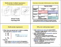
the effect of the former on the latter and not vice versa. Were the assumption not valid, spurious correlation might cause the expert and the trier of fact to reach the wrong conclusion. 41 Figure 1 illustrates this point. In Figure 1(a), the dependent variable, Price, is explained through a multiple regression framework by three explanatory variables, Demand, Cost, and Advertising, with no feedback. In Figure 1(b), however, there is feedback since Price affects Demand, and Demand, Cost, and Advertising affect Price. Cost and Advertising, however, are not affected by Price. As a general rule, there is no direct statistical test for determining the direction of causality. Rather the expert, when asked, should be prepared to defend his or her assumption based on an understanding of the underlying behavior of the firms or individuals involved. Although there is no single approach that is entirely suitable for estimating models when the dependent variable affects one or more explanatory variables, one possibility is for the expert to drop the questionable variable from the regression to determine whether the variable’s exclusion makes a difference. If it does not, the issue becomes moot. Second, the expert can expand the multiple regression model by adding one or more equations that explain the relationship between the explanatory variable in question and the dependent variable.

41. This is especially important in litigation, because it is possible for the defendant (if responsible, for ex ample, for price fixing or discrimination) to affect the values of the explanatory variables and thus to bias the usual statistical tests that are used in multiple regression.

Multiple Regression

433

Figure 1 Feedback 1(a). No Feedback

Demand Price

Cost Advertising

1(b). Feedback Demand Price

Cost Advertising

Suppose, for example, that in a salary-based sex discrimination suit the defendant’s expert considers employer-evaluated test scores to be an appropriate explanatory variable for the dependent variable, salary. If the plaintiff were to provide information that the employer adjusted the test scores in a manner that penalized women, the assumption that salaries were determined by test scores and not that test scores were affected by salaries might be invalid. If it is clearly inappropriate, the test-score variable should be removed from consideration. Alternatively, the information about the employer’s use of the test scores could be translated into a second equation in which a new dependent variable, test score, is related to workers’ salary and sex. A test of the hypothesis that salary and sex affect test scores would provide a suitable test of the absence of feedback. 2. To what extent are the explanatory variables correlated with each other? It is essential in multiple regression analysis that the explanatory variable of interest not be correlated perfectly with one or more of the other explanatory variables. If there were perfect correlation between two variables, the expert could not separate out the effect of the variable of interest on the dependent variable from the effect of the other variable. Suppose, for example, that in a sex discrimination suit a particular form of job experience is determined to be a valid source of high wages. If all men had the requisite job experience and all women

434


did not, it would be impossible to tell whether wage differentials between men and women were due to sex discrimination or differences in experience. When two or more explanatory variables are correlated perfectly—that is, when there is perfect collinearity —one cannot estimate the regression parameters. When two or more variables are highly, but not perfectly, correlated—that is, when there is multicollinearity —the regression can be estimated, but some concerns remain. The greater the multicollinearity between two variables, the less precise are the estimates of individual regression parameters (even though there is no problem in estimating the joint influence of the two variables and all other regression parameters). Fortunately, the reported regression statistics take into account any multicollinearity that might be present.42 It is important to note as a corollary, however, that a failure to find a strong relationship between a variable of interest and a dependent variable need not imply that there is no relationship. 43 A relatively small sample, or even a large sample with substantial multicollinearity, may not provide sufficient information for the expert to determine whether there is a relationship. 3. To what extent are individual errors in the regression model independent? If the parameters of a multiple regression model were calculated using the entire universe of data (the population), the estimates might still measure the model’s population parameters with error. Errors can arise for a number of reasons, including (a) the failure of the model to include the appropriate explanatory variables; (b) the failure of the model to reflect any nonlinearities that might be present; and (c) the inclusion of inappropriate variables in the model. (Of course, fur ther sources of error will arise if a sample of the population is used to estimate the regression parameters.) It is useful to view the cumulative effect of all of these sources of modeling error as being represented by an additional variable, the error term, in the multiple regression model. An important assumption in multiple regression analysis is that the error term and each of the explanatory variables are independent of each other. (If the error term and the explanatory variable are independent, they are not correlated with each other.) To the extent this is the case, the expert can estimate the parameters of the model without bias; the magnitude of the error term will affect the precision with which a model parameter is estimated, but will not cause that estimate to be consistently too high or too low. 42. See Denny v. Westfield State College, 669 F. Supp. 1146, 1149 (D. Mass. 1987) (the court accepted the testimony of one expert that “the presence of multicollinearity would merely tend to overestimate the amount of error associated with the estimate . . . . In other words, P- values will be artificially higher than they would be if there were no multicollinearity present.”) (emphasis added). 43. If a variable of interest and another explanatory variable are highly correlated, dropping the second variable from the regression can be instructive. If the coefficient on the variable of interest becomes significant, a relationship between the dependent variable and the variable of interest is suggested.

Multiple Regression

435

The assumption of independence may be inappropriate in a number of circumstances. In some cases, failure of the assumption makes multiple regression analysis an unsuitable statistical technique; in other cases, modifications or adjustments within the regression framework can be made to accommodate the failure. The independence assumption may fail, for example, in a study of individual behavior over time, in which an unusually high error value in one time period is likely to lead to an unusually high value in the next time period. For example, if an economic forecaster underpredicted this year’s Gross National Product (GNP), he or she is likely to underpredict next year’s as well; the factor that caused the prediction error (e.g., an incorrect assumption about Federal Reserve policy) is likely to be a source of error in the future. Alternatively, the assumption of independence may fail in a study of a group of firms at a particular point in time, in which error terms for large firms are systematically higher than error terms for small firms. For example, an analysis of the profitability of firms may not accurately account for the importance of advertising as a source of increased sales and profits. To the extent that large firms advertise more than small firms, the regression errors would be large for the large firms and small for the small firms. In some cases, there are statistical tests that are appropriate for evaluating the independence assumption.44 If the assumption has failed, the expert should ask first whether the source of the lack of independence is the omission of an important explanatory variable from the regression. If so, that variable should be included when possible, or the potential effect of its omission should be estimated when inclusion is not possible. If there is no important missing explanatory variable, the expert should apply one or more procedures that modify the standard multiple regression technique to allow for more accurate estimates of the regres sion parameters. 45 4. To what extent are the regression results sensitive to individual data points? Estimated regression coefficients can be highly sensitive to particular data points. Suppose, for example, that one data point deviates greatly from its expected value, as indicated by the regression equation, while the remaining data points show little deviation. It would not be unusual in this situation for the co44. In a time-series analysis, the correlation of error values over time, the serial correlation , can be tested (in most cases) using a Durbin-Watson test. The possibility that some disturbance terms are consistently high in magnitude while others are systematically low, heteroscedasticity , can also be tested in a number of ways. See, e.g. , Pindyck & Rubinfeld, supra note 28, at 126–56. 45. When serial correlation is present, a number of closely related statistical methods are appropriate, in cluding generalized differencing (a type of generalized least-squares) and maximum-likelihood estimation. When heteroscedasticity is the problem, weighted least-squares and maximum-likelihood estimation are appropriate. See, e.g. , Pindyck & Rubinfeld, supra note 28, at 126–56. All these techniques are readily available in a number of statistical computer packages. They also allow one to perform the appropriate statistical tests of the significance of the regression coefficients.

436


efficients in a multiple regression to change substantially if the data point were removed from the sample. Evaluating the robustness of multiple regression results is a complex endeavor. Consequently, there is no agreed on set of tests for robustness which analysts should apply. In general, it is important to explore the reasons for unusual data points. If the source is an error in recording data, the appropriate corrections can be made. If all the unusual data points have certain characteristics in common (e.g., they all are associated with a supervisor who consistently gives high ratings in an equal pay case), the regression model should be modified appropriately. One generally useful diagnostic technique is to see to what extent the estimated parameter changes as each data point (or points) in the regression analysis is dropped from the sample. An influential data point—a point that causes the estimated parameter to change substantially—should be studied further to see whether mistakes were made in the use of the data or whether important explanatory variables were omitted. 46 5. To what extent are the data subject to measurement error? In multiple regression analysis it is assumed that variables are measured accurately. 47 If there are measurement errors in the dependent variable, estimates of regression parameters will be less accurate, though they will not necessarily be biased. However, if one or more independent variables are measured with error, the corresponding parameter estimates are likely to be biased, typically toward 0.48 To understand why, suppose that the dependent variable, salary, is measured without error, and the explanatory variable, experience, is subject to measurement error. (Seniority or years of experience should be accurate, but the type of experience is subject to error, since applicants may overstate previous job responsibilities.) As the measurement error increases, the estimated parameter associated with the experience variable will tend toward 0—eventually, there will be no relationship between salary and experience. It is important for any source of measurement error to be carefully evaluated. In some circumstances, little can be done to correct the measurement error problem; the regression results must be interpreted in that light. In other cases, however, measurement errors can be corrected by finding a new, more reliable data source. Finally, alternative estimation techniques (using related variables

46. A more complete and formal treatment of the robustness issue appears in David A. Belsley et al., Regression Diagnostics: Identifying Influential Data and Sources of Collinearity (1980). 47. Inaccuracy can occur not only in the precision by which a particular variable is measured, but also in the precision with which the variable to be measured corresponds to the appropriate theoretical construct spec ified by the regression model. 48. Other coefficient estimates are likely to be biased as well.

Multiple Regression

437

that are measured without error) can be applied to remedy the measurement error problem in some situations. 49

49. See, e.g., Pindyck & Rubinfeld, supra note 28, at 157–79 (discussion of instrumental variables estima tion ).

438


IV. The Expert

Multiple regression analysis is taught to students in an extremely diverse set of fields, including statistics, economics, political science, sociology, psychology, anthropology, public health, and history. Consequently, any individual with substantial training in and experience with multiple regression and other statisti cal methods may be qualified as an expert. 50 A doctoral degree in a discipline that teaches theoretical or applied statistics, such as economics, history, and psychology, usually signifies to other scientists that the proposed expert meets this preliminary test of the qualification process. The decision to qualify an expert in regression analysis rests with the court. Clearly, the proposed expert should be able to demonstrate an understanding of the discipline. Publications relating to regression analysis in peer-reviewed journals, active memberships in related professional organizations, courses taught on regression methods, and practical experience with regression can indicate a professional’s expertise. However, the expert’s background and experience with the specific issues and tools that are applicable to a particular case should also be considered during the qualification process.

50. A proposed expert whose only statistical tool is regression analysis may not be able to judge when a sta tistical analysis should be based on an approach other than regression.

439

V. Presentation of Statistical Evidence

The costs of evaluating statistical evidence can be reduced and the precision of that evidence increased if the discovery process is used effectively. The following questions should be considered in evaluating the admissibility of statistical evidence. 51 These considerations are motivated by two concerns: (1) Has the ex pert provided sufficient information to replicate the multiple regression analysis? (2) Are the methodological choices that the expert made reasonable, or are they arbitrary and unjustified?

A. What Disagreements Exist Regarding Data on Which the Analysis Is Based? In general, a clear and comprehensive statement of the underlying research methodology is a requisite part of the discovery process. The expert should be encouraged to reveal both the nature of the experimentation carried out and the sensitivity of the results to the data and to the methodology. The following are suggestions of a number of useful requirements that can substantially improve the discovery process. 1. To the extent possible, the parties should be encouraged to agree to use a common database. Early agreement on a common database, even if disagreement about the significance of the data remains, can help focus the discovery process on the important issues in the case. 2. A party that offers data to be used in statistical work, including multiple regression analysis, should be encouraged to provide the following to the other parties: (a) a hard copy of the data when available and manageable in size, along with the underlying sources; (b) computer disks or tapes on which the data are recorded; (c) complete documentation of the disks or tapes; (d) computer programs that were used to generate the data (in hard copy, on a computer disk or tape, or both); and (e) documentation of such computer programs.

51. See also David H. Kaye & David A. Freedman, Reference Guide on Statistics § I.B, in this manual.

441

3. A party offering data should make available the personnel involved in the compilation of such data to answer the other parties’ technical questions concerning the data and the methods of collection or compilation. 4. A party proposing to offer an expert’s regression analysis at trial should ask the expert to fully disclose: (a) the database and its sources; 52 (b) the method of collecting the data; and (c) the methods of analysis. When possible, this disclosure should be made sufficiently in advance of trial so that the opposing party can consult its experts and prepare crossexamination. The court must decide on a case-by-case basis where to draw the disclosure line. 5. An opposing party should be given the opportunity to object to a database or to a proposed method of analysis of the database to be offered at trial. Objections may be to simple clerical errors or to more complex issues relating to the selection of data, the construction of variables, and, on occasion, the particular form of statistical analysis to be used. Whenever possible, these objections should be resolved before trial. 6. The parties should be encouraged to resolve differences as to the appropriateness and precision of the data to the extent possible by informal conference. The court should make an effort to resolve differences before trial.

B. What Database Information and Analytical Procedures Will Aid in Resolving Disputes over Statistical Studies? 53 1. The expert should state clearly the objectives of the study, as well as the time frame to which it applies and the statistical population to which the results are being projected. 2. The expert should report the units of observation (e.g., consumers, businesses, or employees). 3. The expert should clearly define each variable. 4. The expert should clearly identify the sample of data being studied, 54 as well as the method by which the sample was obtained.

52. These sources would include all variables used in the statistical analyses conducted by the expert, not simply those variables used in a final analysis on which the expert expects to rely. 53. For a more complete discussion of these requirements, see The Evolving Role of Statistical Assessments as Evidence in the Courts app. F at 256 (Stephen E. Fienberg ed., 1989) (Recommended Standards on Disclosure of Procedures Used for Statistical Studies to Collect Data Submitted in Evidence in Legal Cases). 54. The sample information is important because it allows the expert to make inferences about the under lying population.

442


5. The expert should reveal if there are missing data, whether caused by a lack of availability (e.g., in business data) or nonresponse (e.g., in survey data), and the method used to handle the missing data (e.g., deletion of observations). 6. The expert should report investigations that were made into errors associated with the choice of variables and assumptions underlying the regression model. 7. If samples have been chosen randomly from a population (i.e., probabil ity sampling procedures have been used), 55 the expert should make a good faith effort to provide an estimate of a sampling error, the measure of the difference between the sample estimate of a parameter (such as the mean of a dependent variable under study) and the (unknown) population parameter (the population mean of the variable). 56 8. If probability sampling procedures have not been used, the expert should report the set of procedures that were used to minimize sampling errors.

55. In probability sampling, each representative of the population has a known probability of being in the sample. Probability sampling is ideal because it is highly structured, and in principle, it can be replicated by others. Nonprobability sampling is less desirable because it is often subjective, relying to a large extent on the judgment of the expert. 56. Sampling error is often reported in terms of standard errors or confidence intervals. See infra the Appendix for details.

Multiple Regression

443

Appendix: The Basics of Multiple Regression

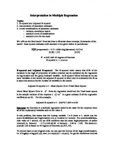
I. Introduction This appendix illustrates, through examples, the basics of multiple regression analysis in legal proceedings. Often, visual displays are used to describe the relationship between variables that are used in multiple regression analysis. Figure 2 is a scatterplot that relates scores on a job aptitude test (shown on the x-axis) and job performance ratings (shown on the y-axis). Each point on the scatterplot shows where a particular individual scored on the job aptitude test and how his or her job performance was rated. For example, the individual represented by Point A in Figure 2 scored 49 on the job aptitude test and had a job performance rating of 62.

Figure 2 Scatterplot 100 •

Job Performance Rating

•

•

•

75 •

A •

50 •

•

• •

25

0

25

50

75

Job Aptitude Test Score

445

100

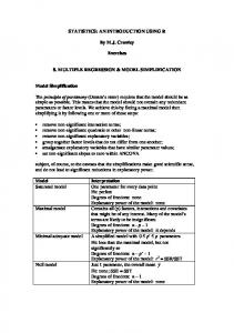
The relationship between two variables can be summarized by a correlation coefficient, which ranges in value from -1 (a perfect negative relationship) to +1 (a perfect positive relationship). Figure 3 depicts three possible relationships between the job aptitude variable and the job performance variable. In Figure 3(a) there is a positive correlation: In general, higher job performance ratings are associated with higher aptitude test scores, and lower job performance ratings are associ ated with lower aptitude test scores. In Figure 3(b) the correlation is negative: Higher job performance ratings are associated with lower aptitude test scores, and lower job performance ratings are associated with higher aptitude test scores. Positive and negative correlations can be relatively strong or relatively weak. If the relationship is sufficiently weak, there is effectively no correlation, as is illustrated in Figure 3(c).

Figure 3 Correlation 3(b). Negative correlation • • • •

• • •

•

•



3(a). Positive correlation

•

•

• • •

•

•

• •

• •




3(c). No correlation

• •

• •

• •

• •


446


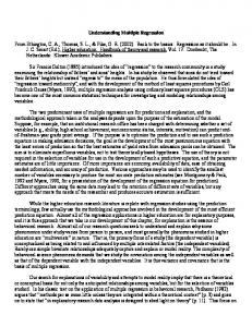
Multiple regression analysis goes beyond the calculation of correlations; it is a method in which a regression line is used to relate the average of one variable— the dependent variable—to the values of other explanatory variables. As a result, regression analysis can be used to predict the values of one variable using the values of others. For example, if average job performance ratings depend on aptitude test scores, regression analysis can use information about test scores to predict job performance. A regression line is the best-fitting straight line through a set of points in a scatterplot. If there is only one explanatory variable, the straight line is defined by the equation: Y = a + bX

In the equation above, a is the intercept of the line with the y-axis when X equals 0, and b is the slope —the amount of vertical change in the line for each unit of change in the horizontal direction. In Figure 4, for example, when the aptitude test score is 0, the predicted (average) value of the job performance rating is the intercept, 18.4. Also, for each additional point on the test score, the job performance rating increases .73 units, which is given by the slope .73. Thus, the estimated regression line is: Yˆ = 18.4 + .73 X

The regression line typically is estimated using the standard method of leastsquares , where the values of a and b are calculated so that the sum of the squared deviations of the points from the line are minimized. In this way, positive deviations and negative deviations of equal size are counted equally, and large deviations are counted more then small deviations. In Figure 4 the deviation lines are vertical because the equation is predicting job performance ratings from aptitude tests scores, not aptitude test scores from job performance ratings.

Multiple Regression

447

Figure 4 Regression Line 100 •


•

•

•

75 •

•

50 •

•

•

•

25

0

25

50

75

100


The important variables that systematically might influence the dependent variable, and for which data can be obtained, typically should be included explicitly in a statistical model. All remaining influences, which should be small individually, but can be substantial in the aggregate, are included in an additional random error term. 57 Multiple regression is a procedure that separates the systematic effects (associated with the explanatory variables) from the random effects (associated with the error term) and also offers a method of assessing the success of the process.

II. Linear Regression Model When there is an arbitrary number of explanatory variables, the linear regression model takes the following form: Y = β0 + β1 X 1 + β2 X 2 +K + β k X k + ε

(1)

where Y represents the dependent variable, such as the salary of an employee, and X 1 . . . Xk represent the explanatory variables (e.g., the experience of each employee and his or her sex, coded as a 1 or 0, respectively). The error term ε represents the collective unobservable influence of any omitted variables. In a 57. It is clearly advantageous for the random component of the regression relationship to be small relative to the variation in the dependent variable.

448


linear regression each of the terms being added involves unknown parameters, β0 , β1, . . . βk ,58 which are estimated by “fitting” the equation to the data using least-squares. Most statisticians use the least-squares regression technique because of its simplicity and its desirable statistical properties. As a result, it also is used frequently in legal proceedings. A. An Example Suppose an expert wants to analyze the salaries of women and men at a large publishing house to discover whether a difference in salaries between employees with similar years of work experience provides evidence of discrimination. 59 To begin with the simplest case, Y, the salary in dollars per year, represents the dependent variable to be explained, and X1 represents the explanatory variable— the number of years of experience of the employee. The regression model would be written: Y = β 0 + β1 X 1 + ε

(2)

In equation (2), β0 and β1 are the parameters to be estimated from the data, and ε is the random error term. The parameter β0 is the average salary of all em ployees with no experience. The parameter β1 measures the average effect of an additional year of experience on the average salary of employees. B. Regression Line Once the parameters in a regression equation, such as equation (1), have been estimated, the fitted values for the dependent variable can be calculated. If we denote the estimated regression parameters, or regression coefficients, for the model in equation (1) by b0 , b1 , . . . b k, the fitted values for Y , denoted Yˆ , are given by: Yˆ = b 0 + b1 X 1 + b 2 X 2 +K b k X k

(3)

Figure 5 illustrates this for the example involving a single explanatory variable. The data are shown as a scatter of points; salary is on the vertical axis and years of experience is on the horizontal axis. The estimated regression line is drawn through the data points. It is given by: 58. The variables themselves can appear in many different forms. For example, Y might represent the loga rithm of an employee’s salary, and X1 might represent the logarithm of the employee’s years of experience. The logarithmic representation is appropriate when Y increases exponentially as X increases—for each unit in crease in X, the corresponding increase in Y becomes larger and larger. For example, if an expert were to graph growth of U.S. population ( Y) over time (t), an equation of the form log( Y) = β 0 + β 1 log( t) might be appropriate. 59. The regression results used in this example are based on data for 1,715 men and women, which were used by the defense in a sex discrimination case against the New York Times that was settled in 1978. Professor Orley Ashenfelter, of the Department of Economics, Princeton University, provided the data.

Multiple Regression

449

Yˆ = $15,000 + $2,000 X 1

(4)

Thus, the fitted value for the salary associated with an individual’s years of experience X1i is given by: Yˆ i = b 0 + b1 X 1 i (at Point B )

The intercept of the straight line is the average value of the dependent variable when the explanatory variable (or variables) is equal to 0; the intercept b 0 is shown on the vertical axis in Figure 5. Similarly, the slope of the line measures the (average) change in the dependent variable associated with a unit increase in an explanatory variable; the slope b1 also is shown. In equation (4), the intercept $15,000 indicates that employees with no experience earn $15,000 per year. The slope parameter implies that each year of experience adds $2,000 to an “average” employee’s salary.

Salary (Thousands of Dollars) (Y)

Figure 5 Goodness-of-Fit •

Residual (Yi - Yi) • A •

30 Si

B •

S i 21

• b 1 = $2,000

One Year • •

b0 •

•

1

2

3

4

5

6

7

Years of Experience (X1)

Now, suppose that the salary variable is related simply to the sex of the employee. The relevant indicator variable, often called a dummy variable , is X2 , which is equal to 1 if the employee is male, and 0 if the employee is female. Suppose the regression of salary Y on X2 yields the following result: Yˆ = $30, 449 + $10,979 X 2

450


The coefficient $10,979 measures the difference between the average salary of men and the average salary of women. 60 1. Regression Residuals For each data point, the regression residual is the difference between the actual and fitted values of the dependent variable. Suppose, for example, that we are studying an individual with three years of experience and a salary of $27,000. According to the regression line in Figure 5, the average salary of an individual with three years of experience is $21,000. Since the individual’s salary is $6,000 higher than the average salary, the residual (the individual’s salary minus the average salary) is $6,000. In general, the residual e associated with a data point, such as Point A in Figure 5, is given by: e = Y i − Yˆ i

Each data point in the figure has a residual, which is the error made by the leastsquares regression method for that individual. 2. Nonlinearities Nonlinear models account for the possibility that the effect of an explanatory variable on the dependent variable may vary in magnitude as the level of the explanatory variable changes. One useful nonlinear model uses interactions among variables to produce this effect. For example, suppose that S = β1 + β 2 SEX + β 3 EXP + β 4 (EXP × SEX ) + ε

(5)

where S is annual salary, SEX is equal to 1 for women and 0 for men, EXP rep resents years of job experience, and ε is a random error term. The coefficient β2 measures the difference in average salary (across all experience levels) between men and women for employees with no experience. The coefficient β3 measures the effect of experience on salary for men (when SEX = 0), and the coefficient β4 measures the difference in the effect of experience on salary between men and women. It follows, for example, that the effect of one year of experience on salary for men is β3 , while the comparable effect for women is β3 + β4 .61

60. To understand why, note that when X2 equals 0, the average salary for women is $30,449 + $10,979 × 0 = $30,449 Correspondingly, when X2 equals 1, the average salary for men is $30,449 + $10,979 × 1 = $41,428 The difference, $41,428 – $30,449, is $10,979. 61. Estimating a regression in which there are interaction terms for all explanatory variables, as in equation (5), is essentially the same as estimating two separate regressions, one for men and one for women.

Multiple Regression

451

III. Interpreting Regression Results To understand how regression results are interpreted, the earlier example associ ated with Figure 5 can be expanded to consider the possibility of an additional explanatory variable—the square of the number of years of experience, X3 . The X3 variable is designed to capture the fact that for most individuals, salaries increase with experience, but eventually salaries tend to level off. The estimated regression line using the third additional explanatory variable, as well as the first explanatory variable for years of experience (X 1 ) and the dummy variable for sex (X2 ), is Yˆ = $14,085 + $2,323 X 1 + $1,675 X 2 − $36 X 3

(6)

The importance of including relevant explanatory variables in a regression model is illustrated by the change in the regression results after the X3 and X2 variables are added. The coefficient on the variable X2 measures the difference in the salaries of men and women while holding the effect of experience constant. The differential of $1,675 is substantially lower than the previously measured differential of $10,979. Clearly, failure to control for job experience in this example leads to an overstatement of the difference in salaries between men and women. Now consider the interpretation of the explanatory variables for experience, X1 and X3 . The positive sign on the X 1 coefficient shows that salary increases with experience. The negative sign on the X 3 coefficient indicates that the rate of salary increase decreases with experience. To see the combined effect of the variables X 1 and X 3 , some simple calculations can be made. For example, consider how the average salary of women (X2 = 0) changes with the level of experience. As experience increases from 0 to 1 year, the average salary increases by $2,251, from $14,085 to $16,336. However, women with 2 years of experience earn only $2,179 more than women with 1 year of experience, and women with 3 years of experience earn only $2,127 more than women with 2 years. Further, women with 7 years of experience earn $28,582 per year, which is only $1,855 more than the $26,727 earned by women with 6 years of experience. 62 Figure 6 illustrates the results; the regression line shown is for women’s salaries; the corresponding line for men’s salaries would be parallel and $1,675 higher.

62. These numbers can be calculated by substituting different values of X1 and X3 in equation (6).

452


Figure 6 Regression Slope

Salary (Thousands of Dollars)

30

20

10

1

2

3

4

5

6

7

Years of Experience

IV. Determining the Precision of the Regression Results Least-squares regression provides not only parameter estimates that indicate the direction and magnitude of the effect of a change in the explanatory variable on the dependent variable, but also an estimate of the reliability of the parameter estimates and a measure of the overall goodness-of-fit of the regression model. Each of these factors is considered in turn. A. Standard Errors of the Coefficients and t-Statistics Estimates of the true but unknown parameters of a regression model are numbers that depend on the particular sample of observations under study. If a different sample were used, a different estimate would be calculated. 63 If the expert continued to collect more and more samples and generated additional estimates, as might happen when new data became available over time, the estimates of each parameter would follow a probability distribution (i.e., the expert could determine the percentage or frequency of the time that each estimate occurs). This probability distribution can be summarized by a mean and a measure of

63. The least-squares formula that generates the estimates is called the least-squares estimator, and its val ues vary from sample to sample.

Multiple Regression

453

dispersion around the mean, a standard deviation, that usually is referred to as the standard error of the coefficient , or the standard error .64 Suppose, for example, that an expert is interested in estimating the average price paid for a gallon of unleaded gasoline by consumers in a particular geographic area of the United States at a particular point in time. The mean price for a sample of ten gas stations might be $1.25, while the mean for another sample might be $1.29, and the mean for a third, $1.21. On this basis, the expert also could calculate the overall mean price of gasoline to be $1.25 and the standard deviation to be $0.04. Least-squares regression generalizes this result, by calculating means whose values depend on one or more explanatory variables. The standard error of a regression coefficient tells the expert how much the parameter estimate is likely to vary from sample to sample. The greater the variation in parameter estimates from sample to sample, the larger the standard error and consequently the less reliable the regression results. Small standard errors imply results that are likely to be similar from sample to sample, while results with large standard errors show more variability. Under appropriate assumptions, the least-squares estimators provide “best” determinations of the true underlying parameters. 65 In fact, least-squares has several desirable properties. First, least-squares estimators are unbiased. Intuitively, this means that if the regression were calculated over and over again with different samples, the average of the many estimates obtained for each coefficient would be the true parameter. Second, least-squares estimators are consistent ; if the sample were very large, the estimates obtained would come close to the true parameters. Third, least-squares is efficient, in that its estimators have the smallest variance among all (linear) unbiased estimators. If the further assumption is made that the probability distribution of each of the error terms is known, statistical statements can be made about the precision of the coefficient estimates. For relatively large samples (often, thirty or more data points will be sufficient for regressions with a small number of explanatory variables), the probability that the estimate of a parameter lies within an interval of 2 standard errors around the true parameter is approximately .95, or 95%. A frequent, although not always appropriate, assumption in statistical work is that the error term follows a normal distribution, from which it follows that the esti mated parameters are normally distributed. The normal distribution has the property that the area within 1.96 standard errors of the mean is equal to 95% of the total area. Note that the normality assumption is not necessary for least64. See David H. Kaye & David A. Freedman, Reference Guide on Statistics § IV.A, in this manual. 65. The necessary assumptions of the regression model include (a) the model is specified correctly; (b) er rors associated with each observation are drawn randomly from the same probability distribution and are inde pendent of each other; (c) errors associated with each observation are independent of the corresponding obser vations for each of the explanatory variables in the model; and (d) no explanatory variable is correlated per fectly with a combination of other variables.

454


squares to be used, since most of the properties of least-squares apply regardless of normality. In general, for any parameter estimate b, the expert can construct an interval around b such that there is a 95% probability that the interval covers the true pa rameter. This 95% confidence interval 66 is given by: b ± 1.96 × ( standard error of b ) 67

(7)

The expert can test the hypothesis that a parameter is actually equal to 0—often stated as testing the null hypothesis—by looking at its t-statistic, which is defined as: t =

b standard error of b

(8)

If the t-statistic is less than 1.96 in magnitude, the 95% confidence interval around b must include 0.68 Because this means that the expert cannot reject the hypothesis that β equals 0, the estimate, whatever it may be, is said to be not statistically significant. Conversely, if the t-statistic is greater than 1.96 in absolute value, the expert concludes that the true value of β is unlikely to be 0 (intuitively, b is “too far” from 0 to be consistent with the true value of β being 0). In this case, the expert rejects the hypothesis that β equals 0 and calls the es timate statistically significant. If the null hypothesis β equals 0 is true, using a 95% confidence level will cause the expert to falsely reject the null hypothesis 5% of the time. Consequently, results often are said to be significant at the 5% level. 69 As an example, consider a more complete set of regression results associated with the salary regression described in equation (6): Yˆ = $14,085 + $2,323 X 1 + $1,675 X 2 − $36 X 3 (1,577) (140) (1, 435) (3.4) t = 8.9 16.5 1.2 −10.8

(9)

The standard error of each estimated parameter is given in parentheses directly below the parameter, and the corresponding t-statistics appear below the standard error values. Consider the coefficient on the dummy variable X2 . It indicates that $1,675 is the best estimate of the mean salary difference between men and women. 66. Confidence intervals are used commonly in statistical analyses because the expert can never be certain that a parameter estimate is equal to the true population parameter. 67. If the number of data points in the sample is small, the standard error must be multiplied by a number larger than 1.96. 68. The t-statistic applies to any sample size. As the sample gets large, the underlying distribution, which is the source of the t -statistic (the student’s t distribution), approximates the normal distribution. 69. A t-statistic of 2.57 in magnitude or greater is associated with a 99% confidence level, or a 1% level of significance, that includes a band of 2.57 standard deviations on either side of the estimated coefficient.

Multiple Regression

455

However, the standard error of $1,435 is large in relation to its coefficient $1,675. Because the standard error is relatively large, the range of possible values for measuring the true salary difference, the true parameter, is great. In fact, a 95% confidence interval is given by: $1,675 ± $1, 435 × 1.96 = $1,675 ± $2, 813

In other words, the expert can have 95% confidence that the true value of the coefficient lies between –$1,138 and $4,488. Because this range includes 0, the effect of sex on salary is said to be insignificantly different from 0 at the 5% level. The t value of 1.2 is equal to $1,675 divided by $1,435. Because this t-statistic is less than 1.96 in magnitude (a condition equivalent to the inclusion of a 0 in the above confidence interval), the sex variable again is said to be an insignificant determinant of salary at the 5% level of significance. Note also that experience is a highly significant determinant of salary, since both the X1 and the X3 variables have t-statistics substantially greater than 1.96 in magnitude. More experience has a significant positive effect on salary, but the size of this effect diminishes significantly with experience. B. Goodness-of-Fit Reported regression results usually contain not only the point estimates of the parameters and their standard errors or t-statistics, but also other information that tells how closely the regression line fits the data. One statistic, the standard error of the regression (SER), is an estimate of the overall size of the regression residuals. 70 An SER of 0 would occur only when all data points lie exactly on the regression line—an extremely unlikely possibility. Other things being equal, the larger the SER, the poorer the fit of the data to the model. For a normally distributed error term, the expert would expect approximately 95% of the data points to lie within 2 SERs of the estimated regression line, as shown in Figure 7 (in Figure 7 the SER is approximately $5,000). R-square (R 2 ) is a statistic that measures the percentage of variation in the dependent variable that is accounted for by all the explanatory variables. 71 Thus, R 2 provides a measure of the overall goodness-of-fit of the multiple regression equation.72 Its value ranges from 0 to 1. An R 2 of 0 means that the explanatory variables explain none of the variation of the dependent variable; an R 2 of 1 means that the explanatory variables explain the variation in the dependent variable perfectly. The R2 associated with equation (9) is .56. This implies that the three explanatory variables explain 56% of the variation in salaries. 70. More specifically, it is a measure of the standard deviation of the regression error e. It sometimes is called the root mean square error of the regression line. 71. The variation is the square of the difference between each Y value and the average Y value, summed over all the Y values. 72. R 2 and SER provide similar information, because R 2 is approximately equal to 1 – SER 2 /Variance of Y.

456


Figure 7 Standard Error of the Regression 2 SERs Regression line

Salary (Y)

2 SERs

Experience (X1)

What level of R 2 , if any, should lead to a conclusion that the model is satisfac tory? Unfortunately, there is no clear-cut answer to this question, since the magnitude of R 2 depends on the characteristics of the data series being studied and, in particular, whether the data vary over time or over individuals. Typically, an R2 is low in cross-sectional studies in which differences in individual behavior are explained. It is likely that these individual differences are caused by many factors that cannot be measured. As a result, the expert cannot hope to explain most of the variation. In time-series studies, in contrast, the expert is explaining the movement of aggregates over time. Since most aggregate time series have substantial growth, or trend, in common, it will not be difficult to “explain” one time series using another time series, simply because both are moving together. It follows as a corollary that a high R 2 does not by itself mean that the variables included in the model are the appropriate ones. As a general rule, courts should be reluctant to rely solely on a statistic such as R2 to choose one model over another. Alternative procedures and tests are available. 73

73. These include F-tests and specification error tests. See Pindyck & Rubinfeld, supra note 28, at 107–13, 149–55, 224–28.

Multiple Regression

457

C. Sensitivity of Least-Squares Regression Results The least-squares regression line can be sensitive to extreme data points. This sensitivity can be seen most easily in Figure 8. Assume initially that there are only three data points, A, B, and C, relating information about X1 to the variable Y. The least-squares line describing the best-fitting relationship between Points A, B, and C is represented by Line 1. Point D is called an outlier because it lies far from the regression line that fits the remaining points. When a new, best-fitting least-squares line is reestimated to include Point D, Line 2 is obtained. Figure 8 shows that the outlier Point D is an influential data point, since it has a dominant effect on the slope and intercept of the least-squares line. Because least squares attempts to minimize the sum of squared deviations, the sensitivity of the line to individual points sometimes can be substantial. 74

Figure 8 Least-Squares Regression Line 2 • D

B • • A

Line 1 • C

What makes the influential data problem even more difficult is that the effect of an outlier may not be seen readily if deviations are measured from the final regression line. The reason is that the influence of Point D on Line 2 is so substantial that its deviation from the regression line is not necessarily larger than the deviation of any of the remaining points from the regression line. 75 Although 74. This sensitivity is not always undesirable. In some cases it may be much more important to predict Point D when a big change occurs than to measure the effects of small changes accurately. 75. The importance of an outlier also depends on its location in the data set. Outliers associated with rela tively extreme values of explanatory variables are likely to be especially influential.

458


they are not as popular as least-squares, alternative estimation techniques that are less sensitive to outliers, such as robust estimation, are available.

V. Reading Multiple Regression Computer Output Statistical computer packages that report multiple regression analyses vary to some extent in the information they provide and the form that the information takes. The following table contains a sample of the basic computer output that is associated with equation (6).

Table 1 Regression Output Dependent Variable: Y

SSE

62346266124

F- Test

174.71

DFE

561

Prob > F

0.0001

MSE

111134164

R2

0.5560

DF

Parameter Estimate

Standard Error

t-stat

Prob > | t|

Intercept

1

14084.89

1577.484

8.9287

.0001

X1

1

1675.11

1435.422

1.1670

.2437

X2

1

2323.17

140.70

16.5115

.0001

X3

1

-36.71

3.41

-10.7573

.0001

Variable

Note: SSE = sum of squared errors; DFE = degrees of freedom associated with the error term; MSE = mean square error; DF = degrees of freedom; t-stat = t-statistic; Prob = probability.

Beginning with the lower portion of Table 1, note that the parameter estimates, the standard errors, and the t-statistics match the values given in equation (9). 76 The variable “Intercept” refers to the constant term β0 in the regression. The column DF represents degrees of freedom . The “1” signifies that when the computer calculates the parameter estimates, each variable that is added to the linear regression adds an additional constraint that must be satisfied. The column labeled “Prob > |t|” lists the two-tailed p-values associated with each estimated parameter; the p-value measures the observed significance level—the probability of getting a test statistic as extreme or more extreme than the observed number if the model parameter is in fact 0. The very low p-values on the variables X2 and X3 imply that each variable is statistically significant at less than the 1% level—both highly significant results. On the contrary, the X 1 coefficient is only significant at the 24% level, implying that it is insignificant at the traditional 5% level. Thus, the expert cannot reject with confidence the null hypoth-

76. Computer programs give results to more decimal places than are meaningful. This added detail should not be seen as evidence that the regression results are exact.

Multiple Regression

459

esis that salaries do not differ by sex after the expert has accounted for the effect of experience. The top portion of Table 1 provides data that relate to the goodness-of-fit of the regression equation. The sum of squared errors (SSE) measures the sum of the squares of the regression residuals—the sum that is minimized by the leastsquares procedure. The degrees of freedom associated with the error term (DFE) is given by the number of observations minus the number of parameters that were estimated. The mean square error (MSE) measures the variance of the error term (the square of the standard error of the regression). MSE is equal to SSE divided by DFE. The R 2 of .556 indicates that 55.6% of the variation in salaries is explained by the regression variables, X1 , X2 , and X3 . Finally, the F-test is a test of the null hy pothesis that all regression coefficients (except the intercept) are jointly equal to 0—that there is no association between the dependent variable and any of the explanatory variables. This is equivalent to the null hypothesis that R 2 is equal to 0. In this case, the F-ratio of 174.71 is sufficiently high that the expert can reject the null hypothesis with a very high degree of confidence (i.e., with a 1% level of significance).

VI. Forecasting In general, a forecast is a prediction made about the values of the dependent variable using information about the explanatory variables. Often, ex ante fore casts are performed; in this situation, values of the dependent variable are predicted beyond the sample (e.g., beyond the time period in which the model has been estimated). However, ex post forecasts are frequently used in damage analyses. 77 An ex post forecast has a forecast period such that all values of the dependent and explanatory variables are known; ex post forecasts can be checked against existing data and provide a direct means of evaluation. For example, to calculate the forecast for the salary regression discussed above, the expert uses the estimated salary equation: Yˆ = $14,085 + $2,323 X 1 + $1,675 X 2 − $36 X 3

(10)

To predict the salary of a man with two years experience, the expert calculates: Yˆ (2) = $14,085 + $2,323 × 2 + $1,675 − $36 × 2 2 = $20,262

(11)

77. Frequently, in cases involving damages, the question arises as to what the world would have been like had a certain event not taken place. For example, in a price-fixing antitrust case, the expert can ask what the price of a product would have been had a certain event associated with the price-fixing agreement not oc curred. If prices would have been lower, the evidence suggests impact. If the expert can predict how much lower they would have been, the data can help the expert develop a numerical estimate of the amount of dam ages.

460


The degree of accuracy of both ex ante and ex post forecasts can be calculated provided that the model specification is correct and the errors are normally distributed and independent. The statistic is known as the standard error of forecast (SEF). The SEF measures the standard deviation of the forecast error that is made within a sample in which the explanatory variables are known with certainty. 78 The SEF can be used to determine how accurate a given forecast is. In equation (11), the SEF associated with the forecast of $20,262 is approximately $5,000. If a large sample size is used, the probability is roughly 95% that the predicted salary will be within 1.96 standard errors of the forecasted value. In this case, the appropriate 95% interval for the prediction is $20,262 ± $5,000 × 1.96 ($10,822 to $30,422). Because the estimated model does not explain salaries effectively, the SEF is large, as is the 95% interval. A more complete model with additional explanatory variables would result in a lower SEF and a smaller 95% interval for the prediction. There is a danger when using the SEF, which applies to the standard errors of the estimated coefficients as well. The SEF is calculated on the assumption that the model includes the correct set of explanatory variables and the correct functional form. If the choice of variables or the functional form is wrong, the estimated forecast error may be misleading; in some cases, it may be smaller, perhaps substantially smaller, than the true SEF; in other cases, it may be larger, for example, if the wrong variables happen to capture the effects of the correct variables.

78. There are actually two sources of error implicit in the SEF. The first source arises because the esti mated parameters of the regression model may not be exactly equal to the true regression parameters. The sec ond source is the error term itself; when forecasting, the expert typically sets the error equal to 0 when a turn of events not taken into account in the regression model may make it appropriate to make the error positive or negative.

Multiple Regression

461

Salary (Y)

Figure 9 Standard Error of Forecast

} 2 SERs

} 2 SEFs

Experience (X1)

The difference between the SEF and the SER is shown in Figure 9. The SER measures deviations within the sample. The SEF is more general, since it calcu lates deviations within or without the sample period. In general, the difference between the SEF and the SER increases as the values of the explanatory variables increase in distance from the mean values. Figure 9 shows the 95% prediction interval created by the measurement of 2 SEFs about the regression line.

462


Glossary of Terms

The following terms and definitions are adapted from a variety of sources, including A Dictionary of Epidemiology (John M. Last ed., 1983) and Robert S. Pindyck & Daniel L. Rubinfeld, Econometric Models & Economic Forecasts (3d ed. 1991). Alternative Hypothesis. See Hypothesis Test. Association. The degree of statistical dependence between two or more events or variables. Events are said to be associated when they occur more frequently together than one would expect by chance. Bias. Any effect at any stage of investigation or inference tending to produce results that depart systematically (either too high or too low) from the true values. A biased estimator of a parameter differs on average from the true parameter. Coefficient. An estimated regression parameter. Confidence Interval. An interval that contains a true regression parameter with a given degree of confidence. Consistent Estimator. An estimator that tends to become more and more accurate as the sample size grows. Correlation. A statistical means of measuring the association between variables. Two variables are correlated positively if, on average, they move in the same direction; two variables are correlated negatively if, on average, they move in opposite directions. Cross-Section Analysis. A type of multiple regression analysis in which each data point is associated with a different unit of observation (e.g., an individual or a firm) measured at a particular point in time. Degrees of Freedom. The number of observations in a sample minus the number of estimated parameters in a regression model. A useful statistic in hypothesis testing. Dependent Variable. The variable to be explained or predicted in a multiple regression model.

463

Dummy Variable. A variable that takes on only two values, usually 0 and 1, with one value indicating the presence of a characteristic, attribute, or effect and the other value indicating absence. Efficient Estimator. An estimator of a parameter that produces the greatest preci sion possible. Error Term. A variable in a multiple regression model that represents the cumulative effect of a number of sources of modeling error. Estimate. The calculated value of a parameter based on the use of a particular sample. Estimator. The sample statistic that estimates the value of a population parameter (e.g., a regression parameter); its values vary from sample to sample. Ex Ante Forecast. A prediction about the values of the dependent variable that go beyond the sample; consequently, the forecast must be based on predictions for the values of the explanatory variables in the regression model. Explanatory Variable. A variable that partially explains or predicts the movement of a dependent variable. Ex Post Forecast. A prediction about the values of the dependent variable made during a period in which all the values of the explanatory and dependent variables are known. Ex post forecasts provide a useful means of evaluating the fit of a regression model. F-test. A statistical test (based on an F-ratio) of the null hypothesis that a group of explanatory variables are jointly equal to 0. When applied to all the explana tory variables in a multiple regression model, the F -test becomes a test of the null hypothesis that R 2 equals 0. Feedback. When changes in an explanatory variable affect the values of the de pendent variable, and changes in the dependent variable also affect the explanatory variable. When both effects occur at the same time, the two variables are described as being determined simultaneously. Fitted Value. The estimated value for the dependent variable; in a linear regression this value is calculated as the intercept plus a weighted average of the values of the explanatory variables, with the estimated parameters used as weights. Heteroscedasticity. When the disturbance or error associated with a multiple regression model has a nonconstant variance; that is, the error values associated with some observations are typically high, whereas the values associated with other observations are typically low. Hypothesis Test. A statement about the parameters in a multiple regression model. The null hypothesis may assert that certain parameters have speci-

464


fied values or ranges; the alternative hypothesis would specify other values or ranges. Independence. When two variables are not correlated with each other (in the population). Independent Variable. An explanatory variable that affects the dependent variable but is not affected by the dependent variable. Influential Data Point. A data point whose addition to a regression sample causes one or more estimated regression parameters to change substantially. Interaction Variable. The product of two explanatory variables in a regression model. Used in a particular form of nonlinear model. Intercept. The value of the dependent variable when each of the explanatory variables takes on the value of 0. Least-Squares. A common method for estimating regression parameters. Leastsquares minimizes the sum of the squared differences between the actual values of the dependent variable and the values predicted by the regression equation. Linear Model. A model having the property that the magnitude of the change in the dependent variable associated with the change in any of the explanatory variables is the same no matter what the level of that variable. Linear Regression. A regression model in which the effect of a change in each of the explanatory variables on the dependent variable is the same, no matter what the values of those explanatory variables. Mean (Sample). An average of the outcomes associated with a probability distribution, where the outcomes are weighted by the probability that each will occur. Mean Square Error (MSE). The estimated variance of the regression error, calculated as the average of the sum of the squares of the regression residuals. Model. A representation of an actual situation. Multicollinearity. Arises in multiple regression analysis when two or more variables are highly correlated. Substantial multicollinearity can cause regression parameters to be estimated imprecisely, as reflected in relatively high standard errors. Multiple Regression Analysis. A statistical tool for understanding the relationship between two or more variables. Multivariate Analysis. A set of techniques used to study the variation in several variables simultaneously.

Multiple Regression

465

Nonlinear Model. A model having the property that changes in explanatory variables will have differential effects on the dependent variable as the values of the explanatory variables change. Normal Distribution. A bell-shaped probability distribution having the property that about 95% of the distribution lies within two standard deviations of the mean. Null Hypothesis. In regression analysis the null hypothesis states that the results observed in a study with respect to a particular variable are no different from what might have occurred by chance, independent of the effect of that variable. See Hypothesis Test. One-Tailed Test. A hypothesis test in which the alternative to the null hypothesis that a parameter is equal to 0 is for the parameter to be either positive or negative, but not both. Outlier. A data point that is more than some appropriate distance from a regression line that is estimated using all the other data points in the sample. p-Value. The probability of getting a test statistic as extreme or more extreme than the observed value. The larger the p-value, the more likely the null hypothesis is true. Parameter. A numerical characteristic of a population or a model. Perfect Collinearity. When two (or more) variables are explanatory variables are correlated perfectly. Population. All the units of interest to the researcher; also, universe. Practical Significance. Substantive importance. Statistical significance does not ensure practical significance, since, with large samples, small differences can be statistically significant. Probability Distribution. The process that generates the values of a random vari able. A probability distribution lists all possible outcomes and the probability that each will occur. Probability Sampling. A process by which a sample of a population is chosen so that each observation has a known probability of being selected. Random. Governed by chance; not completely determined by other factors. Random Error. Random error (sampling error) is due to chance when the result obtained in the sample differs from the result that would be obtained if the entire population were studied. Regression Coefficient. The estimate of a population parameter obtained from a regression equation that is based on a particular sample; also, regression parameter.

466


Residual. The difference between the actual value of a dependent variable and the value predicted by the regression equation. Robust. A statistic or procedure that does not change much when data or as sumptions are slightly modified. Robust Estimation. An alternative to least-squares estimation that is less sensitive to outliers. R-Square ( R2 ). A statistic that measures the percentage of the variation in the dependent variable that is accounted for by all of the explanatory variables in a regression model. R-square is the most commonly used measure of goodness-of-fit of a regression model. Sample. A set of units selected for a study; a subset of a population. Sampling Error. A measure of the difference between the sample estimate of a parameter and the population parameter. Scatterplot. A graph showing the relationship between two variables in a study; each dot represents one subject. One variable is plotted along the horizontal axis; the other variable is plotted along the vertical axis. Serial Correlation. The correlation of the values of regression errors over time. Slope. The change in the dependent variable associated with a 1-unit change in an explanatory variable. Spurious Correlation. When two variables are correlated, but one is not the cause of the other. Standard Deviation. The square root of the variance of a random variable. The variance is a measure of the spread of a probability distribution about its mean; it is calculated as a weighted average of the squares of the deviations of the outcomes of a random variable from its mean. Standard Error of the Coefficient; Standard Error. A measure of the variation of a parameter estimate or coefficient about the true parameter. The standard error is a standard deviation that is calculated from the probability distribution of estimated parameters. Standard Error of Forecast (SEF). An estimate of the standard deviation of the forecast error; it is based on forecasts made within a sample in which the values of the explanatory variables are known with certainty. Standard Error of the Regression (SER). An estimate of the standard deviation of the regression error; it is calculated as an average of the squares of the residuals associated with a particular multiple regression analysis. Statistical Significance. Used to evaluate the degree of association between a dependent variable and one or more explanatory variables. If the calculated pvalue is smaller than 5%, the result is said to be statistically significant (at the

Multiple Regression

467

5% level). If p is less than 5%, the result is statistically insignificant (at the 5% level). t-Statistic. A test statistic that describes how far an estimate of a parameter is from its hypothesized value (i.e., given a null hypothesis). If a t-statistic is sufficiently large (in absolute magnitude), an expert can reject the null hypothesis. t-Test. A test of the null hypothesis that a regression parameter takes on a particular value, usually 0. The test is based on the t -statistic. Time-Series Analysis. A type of multiple regression analysis in which each data point is associated with a particular unit of observation (e.g., an individual or a firm) measured at different points in time. Two-Tailed Test. A hypothesis test in which the alternative to the null hypothesis that a parameter is equal to 0 is for the parameter to be either positive or negative, or both. Variable. Any attribute, phenomenon, condition, or event that can have different values. Variable of Interest. The explanatory variable that is the focal point of a particular study or legal issue. Weighting. Weighting is used when statistics such as the mean and standard deviation are calculated. If ten observations are equally likely to occur, then each is weighted 0.1 when the appropriate statistics are calculated. However, if the first five observations are three times as likely to occur as the second five, the first five receive weights of 0.15, and the second five receive weights of 0.05. (In each case the sum of the weights is 1.0.)

468


References on Multiple Regression

Thomas J. Campbell, Regression Analysis in Title VII Cases: Minimum Standards, Comparable Worth, and Other Issues Where Law and Statistics Meet, 36 Stan. L. Rev. 1299 (1984). Arthur P. Dempster, Employment Discrimination and Statistical Science, 3 Stat. Sci. 149 (1988). The Evolving Role of Statistical Assessments as Evidence in the Courts (Stephen E. Fienberg ed., 1989). Michael O. Finkelstein, The Judicial Reception of Multiple Regression Studies in Race and Sex Discrimination Cases, 80 Colum. L. Rev. 737 (1980). Michael O. Finkelstein & Hans Levenbach, Regression Estimates of Damages in Price-Fixing Cases , Law & Contemp. Probs., Autumn 1983, at 145. Franklin M. Fisher, Statisticians, Econometricians, and Adversary Proceedings, 81 J. Am. Stat. Ass’n 277 (1986). Franklin M. Fisher, Multiple Regression in Legal Proceedings , 80 Colum. L. Rev. 702 (1980). Joseph L. Gastwirth, Methods for Assessing the Sensitivity of Statistical Comparisons Used in Title VII Cases to Omitted Variables, 33 Jurimetrics J. 19 (1992). Note, Beyond the Prima Facie Case in Employment Discrimination Law: Statistical Proof and Rebuttal, 89 Harv. L. Rev. 387 (1975). Daniel L. Rubinfeld, Econometrics in the Courtroom, 85 Colum. L. Rev. 1048 (1985). Daniel L. Rubinfeld & Peter O. Steiner, Quantitative Methods in Antitrust Litigation, Law & Contemp. Probs., Autumn 1983, at 69. Symposium, Statistical and Demographic Issues Underlying Voting Rights Cases , 15 Evaluation Rev. 659 (1991).

469

Reference Guide on Multiple Regression

Reference Guide on Multiple Regression

Suggest Documents

6: Regression and Multiple Regression

REGRESSION ON DUMMY VARIABLES Reference : Gujarati ...

Multivariate Multiple Regression Analysis Based on Principal ...

Multivariate multiple regression

Multiple Regression

Interpretation in Multiple Regression

Exercise 8: Multiple Regression

Understanding Multiple Regression - UMdrive

MULTIPLE REGRESSION BASICS

Multiple Linear Regression - Statistics

Multiple Linear Regression - Statistics

Multiple Neutral Regression

Introduction to Multiple Regression

Review of Multiple Regression

Introduction to Multiple Regression

Reference Guide on DNA Evidence

Guide to using Multiple Regression in Excel - Pacific Northwest ...

Survival Guide Basic Multiple Regression in Minitab.pdf - Google Drive

Product Reference Guide Product Reference Guide 2009

Geary on Inference in Multiple Regression and on Closeness ... - TARA

REFERENCE GUIDE

Multiple Regression Hidden Markov Models

a Multiple Regression Approach

Multivariate-multiple circular regression