Stochastic Dynamic Programming for Long Term

9th International Conference on Probabilistic Methods Applied to Power Systems KTH, Stockholm, Sweden – June 11-15, 2006

1

Stochastic Dynamic Programming for Long Term Hydrothermal Scheduling Considering Different Streamflow Models T. G. Siqueira, M. Zambelli, M. Cicogna, M. Andrade, S. Soares.

Abstract—This paper is concerned with the performance of stochastic dynamic programming for long term hydrothermal scheduling. Different streamflow models progressively more complex have been considered in order to identify the benefits of increasing sophistication of streamflow modeling on the performance of stochastic dynamic programming. The first and simplest model considers the inflows given by their average values; the second model represents the inflows by independent probability distribution functions; and the third model adopts a Markov chain based on a lag-one periodical auto-regressive model. The effects of using different probability distribution functions have been also addressed. Numerical results for a hydrothermal test system composed by a single hydro plant have been obtained by simulation with Brazilian inflow records. Index Terms— streamflow models, long term hydrothermal scheduling, Markov chain, stochastic dynamic programming.

I. NOMENCLATURE LTHS: Long Term Hydrothermal Scheduling. DP: Dynamic Programming. DDP: Deterministic Dynamic Programming. SDP: Stochastic Dynamic Programming. ISDP: Independent Stochastic Dynamic Programming. DSDP: Dependent Stochastic Dynamic Programming. II. INTRODUCTION

T

he long term hydrothermal scheduling (LTHS) problem aims to determine, for each stage (month) of the planning period (years), the amount of generation at each hydro and thermal plant which attends the load demand and minimizes the expected operation cost along the planning period respecting the involved operational constraints [1]. The decision process is made more challenging by the uncertainty of natural streamflows. Stochastic dynamic programming (SDP) has been the most applied technique to solve the LTHS problem since it can handle the non-linear and non-convexity characteristics of hydro plant production and can deal with inflows as random variables described by probability distributions [2]-[3]. Although limited by the so-called “curse of dimensionality”, since its computational burden increases exponentially with the number of hydro plants, the SDP approach has been used in real hydrothermal systems through the aggregation of the hydro system into a composite model [4].

In the SDP approach for LTHS, the random variable (inflow) can be represented through different models. The simplest one is to represent the inflow by its average value, which in practice corresponds to converting the problem into a deterministic one. Another model more commonly used is the independent model, which considers the inflows as independent random variables without time correlation. Finally, a more sophisticated model is the dependent model, which represents the inflow through a Markov chain based on a lag-one periodical auto regressive model. Besides the time correlation of the inflow series, the choice of the probability distribution of the inflows is another aspect that may affect the SDP performance in LTHS. The periodically stationary Gaussian distribution is the most often distribution considered [10]. However, periodically stationary distributions do not properly represent characteristics such as asymmetry and the non-steady behavior of the variance originated by climate changes (dry periods present lower variance whereas humid periods present higher variances). Consequently one should also consider the possibility of the inflows be approximated by different density distribution such as normal, together with the box-cox transformation, and comparing this model with the particular cases where lognormal and periodically stationary distributions are used [8][9]. This paper compares the performance of different SDP models in LTHS for systems composed by a single hydro plant. Although simple, this configuration summarizes the essence of hydrothermal scheduling, besides being adopted in many systems through the aggregation of the hydro system into a composite model [3]. Numerical tests have been progressively performed through simulation in order to evaluate the benefits of increasing sophistication of inflow modeling and density probability adjustments. Features and sensitivities of the different models are discussed. III. FORMULATION OF THE LTHS PROBLEM The LTHS problem, in the deterministic case and considering one hydrothermal plant, can be formulated as a nonlinear programming problem given by:

© Copyright KTH 2006

T −1

min ∑ Ψt (d t − ht ) t =1

ht = k .[φ (vt ) − θ (ut )].rt

(1) (2)

9th International Conference on Probabilistic Methods Applied to Power Systems KTH, Stockholm, Sweden – June 11-15, 2006

ut = rt + st

(3)

vt = vt −1 + (it − ut ) β

2

of the following recursive equation (18) at each stage t [6], [7], [12].

αt −1 (vt −1 ) = min {Cp + C f }

(4)

ut ∈Ut

(18)

vt ∈ Vt

(5)

ut ∈ U t

(6)

rt ∈ Rt

(7)

st ≥ 0

stage t until the end of the planning period;

(8)

cost, is the cost associated with the thermal generation necessary to complement hydro generation in the attainment of the energy demand in the stage t; and C f , called future

where: T : planning period; t : index of planning stages; Ψt (.) : thermal cost function at stage t [$]; d t : energy demand at stage t [MW]; ht : hydro generation at stage t [MW]; k : average specific efficiency [MW/(m3/s)m] φ (vt ) : forebay elevation at stage t [m];

C p = Ψt (dt − ht )

where

α t (vt )

C p , called present

cost, represents the cost associated with saving water for the future. In the deterministic DP approach (DDP), the inflow variable is assumed known as the mean historical value it . The future cost function

θ (u t ) : tailrace elevation at stage t [m];

rt : water discharged at stage t [m³/s]; it : inflow at stage t [m³/s]; vt : reservoir volume at the end of stage t [hm3];

(19) is the optimal operation cost from state vt at

C f is given by: C f = α t (vt )

(20)

vt = vt −1 + (it + ut ) β

(21)

Fig. 1 shows the DDP decision process.

ut : water released at stage t [m³/s];

st : water spilled at stage t [m³/s]; β : conversion factor;

Vt , U t and Rt : feasible sets representing bounds for the variables vt , u t , and rt , respectively. Since spillage does not produce energy, and therefore does not reduce thermal costs, it works as a slack variable that can be different from zero only if the discharge is in its maximum value. Otherwise a better solution can always be obtained by changing spillage for discharge. Therefore, assuming that rt = min{u t , r

max

} , problem (1)-(8) can be Fig. 1. DDP scheme. reformulated only in terms of variables vt (storage variable) In the independent SDP approach (ISDP) there is no time correlation between the inflows. The recursion equation and u t (released water variable). If the inflows are represented by their average values, the solution of problem (1)-(8) can be obtained by deterministic dynamic programming (DDP). However, if the inflows are considered as random variables, the objective turns out to be the minimization of the expected value of (1) with respect to it , and the solution is obtained by SDP.

remains as (18)-(19) and its future cost function is given by (22)-(23). N

C f = ∑αt (vtk ). pk

(22)

vtk = vt −1 + (itk + ut ) β

(23)

k =1

The state variable is represented only by the reservoir storage and the probabilities pk are calculated from the

IV. DYNAMIC PROGRAMMING For solving problem (1)-(8) by DP the optimization process is based on a previous knowledge of the future possibilities and its consequences, satisfying the Bellman optimality principle [5]. The DP algorithm is performed by the backward resolution

probability density function

f (it ) of the random variable it .

The solution process starts at the final stage T , where the cost α T (vT ) is supposed to be known, and goes back until the initial stage t = 0 , according to the recursive equation (18)-

© Copyright KTH 2006

9th International Conference on Probabilistic Methods Applied to Power Systems KTH, Stockholm, Sweden – June 11-15, 2006

(19) and (22)-(23), where C p is the present cost at stage t and C f is the optimal expected future cost until the end of the planning period. Fig. 2 illustrates the calculation scheme of the ISDP approach. Note that DDP can be viewed as a subtype of the ISDP method were the probability associated with the inflow is one for the mean inflow value it and zero for any other value.

3

In the next section the inference of the probabilities of inflows will be discussed for the independent and dependent cases, considering the normal, lognormal and normal with Box Cox transformed data density functions. V. INFLOW MODELING In this section one presents the three densities distribution function used in the inflow modeling for the dynamic programming politics. The first density distribution considered is the Normal distribution; the second one is the Box-Cox family transformation, which includes the lognormal one. A. Normal distribution The normal distribution is the most important one in the study of probabilities and statistics. Various natural phenomena follow the gaussian distribution. Let ir ,m represent the inflow data for months m = 1, K ,12 and years r = 1, K , n . The normal conditional distribution can be written as (9), where µ m|m −1 and σ m|m −1 represent the

Fig. 2. ISDP scheme.

When the inflows are assumed as correlated in time according to a Markov chain [10], leading to the dependent SDP approach (DSDP), the state variable changes to include the inflow of the previous stage, the probabilities p kj are now calculated from the conditional probability density function

f (it / it −1 ) and the recursive equation is modified to:

αt −1 (vt −1 , itj−1 ) = Min {C p + C f } ut ∈Ut

conditional mean and standard deviation given by (10) and (11).

 (ir,m − µm|m−1 )2  f (ir,m | ir,m−1 ) = exp−  (9) 2σm2|m−1   2πσm|m−1 σ µ m|m −1 = µ m + ρ m m (ir ,m −1 − µ m −1 ) σ m −1 (10) 1

(24)

σ m|m−1= σ m (1 − ρ m2 )

(25)

These parameters can be evaluated if the previous inflows ir ,m −1 , the normal parameters ( µ m and σ m ), and the lag-1

(11)

N

C f = ∑ α t (vt , itk ). p kj k =1

Indexes k and j are associated with the discrete inflow variables it and it −1 , respectively, as seen in Fig. 3.

correlation ρ m between two consecutive data are known. The parameters of the conditional normal density used in (10)-(11) can be estimated using the historical data, according to (12)-(14).

µm = σm =

ρm =

1 n ∑ ir ,m n r =1

1 n 2 ∑ (ir ,m − µ m ) n − 1 r =1

∑ (ir ,m − µ m )(ir ,m −1 − µ m −1 ) σ m σ m −1

(12)

(13)

n r =1

(14)

When the SDP with independent inflows is considered there is no correlation between the inflows, i.e., ρ m = 0 . B. The Box-Cox transformation Fig. 3. DSDP scheme.

© Copyright KTH 2006

9th International Conference on Probabilistic Methods Applied to Power Systems KTH, Stockholm, Sweden – June 11-15, 2006 TABLE I HYDRO PLANTS OPERATIONAL DATA

When the hypothesis of normal distribution is not valid, at least in an approximate manner, an alternative is to apply the Box-Cox transformation to the historical inflow data ir ,m , [8], [9]. This transformation family has a particular case for logarithmical transformations where the historical inflows follow a lognormal distribution. The family of Box-Cox transformations is given by (15).

Tr ,m

 (irλ,m − 1)  = λ  ln(ir ,m )

if

λ≠0

if

λ=0

(15)

4

Plant

Sobradinho

Furnas

Installed capacity (MW) Average specific efficiency (MW/(m3/s)m) Max Discharge (m3/s) Min/Max volume (hm3)

1050

1312

0.009025

0.008633

4183.2

1616

5447 / 34116

5733 / 22950

The inverse data transformation is given by:

(λT + 1) 1λ T r ,m =  r ,m  exp(Tr ,m ) for m = 1,K,12 e r = 1, K , n . −1

if

λ≠0

if

λ=0

(16)

In (15) for λ = 0 the inflows present a lognormal conditional distribution. This is the hypothesis that has been adopted in the stochastic models used by the Brazilian ISO. Finally, one can obtain the conditional probability of the inflow ir ,m | ir ,m −1 occurs, Pm|m −1 for each discrete interval ( Ar , m , B r , m ) using standard normal variable:

z r ,m = where

µm

and

σm

Tr ,m − µ m

σm

(17)

are the mean and standard deviation of

In all methods the state and control variables were discretized into 60 and 30 values, respectively. For the SDP, the inflow variable was discretized into 10 possible values. The box-cox parameters, λ , used in the SDP for Sobradinho and Furnas hydro plants were obtained from the maximum likelihood method [13]. They were equal to –0.09 and –0.115, respectively. The operation policies were implemented and simulated in a monthly basis throughout the inflow historical sequence, which in this case ranges begins in 1931. All the constraints (2)-(8) presented in the formulation of the optimization problem have been considered in the simulation. Tables II and III show the simulation results of two case studies with Sobradinho and Furnas hydro plants, where

h and std h are the average hydro generation and its standard deviation and C is the average cost.

the transformed data Tr ,m .

TABLE II SIMULATION RESULTS OF SOBRADINHO

VI. RESULTS In order to assess the influence of these inflow models in SDP for LTHS, numerical tests were performed for a hydrothermal system composed by a single hydro plant operating with a thermal plant with the same power capacity. Although simple, this configuration summarizes the essence of hydrothermal scheduling, besides being adopted in many systems through the aggregation of the hydro system into a composite model [3]. Sobradinho hydro plant located in the northeastern region of Brazil (São Francisco river) and Furnas (Grande river) hydro plant in the southeastern region of Brazil have been chosen for this case study. In the comparison of the inflow modeling in SDP, the normal, lognormal and normal with Box-Cox transformation data distributions were considered. The energy demand in MW was considered constant and equal to the system installed capacity. The thermal cost was considered as Ψt = 0.5( d − ht ) . The forebay φ ( xt ) and 2

tailrace θ (u t ) elevations were calculated by 4th degree polynomial functions. Table I shows the main operational data of the hydro plants considered.

h (MW) Std h (MW) Approach DDP 570,70 173,94 Normal 564,57 178,40 ISDP Log-Normal 565,50 175,41 Box-Cox 564,93 177,80 Normal 572,30 174,16 DSDP Log-Normal 573,23 165,05 Box-Cox 572,88 164,83

C ($) 129976 133713 132738 133434 129243 127257 127389

TABLE III SIMULATION RESULTS OF FURNAS

h (MW) Std h (MW) Approach DDP 718,80 182,80 Normal 715,00 173,30 ISDP Log-Normal 714,20 170,91 Box-Cox 714,60 171,44 Normal 717,90 179,46 DSDP Log-Normal 717,10 173,95 Box-Cox 716,30 173,55

© Copyright KTH 2006

C ($) 192604 193176 193282 193146 192563 192087 192451

9th International Conference on Probabilistic Methods Applied to Power Systems KTH, Stockholm, Sweden – June 11-15, 2006

Furnas

Reservoir Storage (%)

120

100

80

60

Sobradinho 120

Reservoir Storage (%)

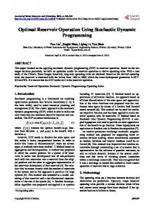
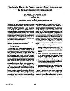
First of all, one can conclude from the simulation results that the deterministic and stochastic approaches have provided quite similar performance in both case studies. Differences are quite small in terms of hydro generation and cost which means that the stochastic models considered do not provide significant improvement in DP for LTHS. This result is very important since deterministic approaches, on the contrary of the stochastic ones, can handle multi reservoir systems without the need of any modeling manipulation. It is very surprising that DDP has provided better results in terms of higher hydro generation and lower cost than ISDP for both case studies. Indeed, DDP has given quite similar results when compared with DSDP in all case studies. From the results one can also conclude that DSDP furnishes slightly better performance than ISDP for both case studies. The improvement is due to an increase on average hydro generation and, for the Sobradinho case study, some reduction on the standard deviation of hydro generation. It is important to note that the influence of the density distribution functions are in general quite small for both SDP approaches. The only meaninful influence is observed in the case of the DSDP approach for the Furnas case study. In this case, the Box-Cox transformation, including the lognormal one, have given better results than the normal one. Fig. 4 shows the water reservoir storage trajectories of Furnas hydro plant during the late 50s, which includes the dryest period of the historical records, obtained with simulation using the DDP and SDP approaches with normal density function. The storage trajectories were very similar, and for this specific period, DDP has presented better performance than SDP methods since the reservoir operate with higher storage, and therefore, efficiency. Fig. 5 shows the performance of the DSDP for the 50th using the three density functions considered in this study for Sobradinho hydro plant. In this case, DSDP using the box-cox probability function family provided almost the same performance while DDP depleted more water and presented lower storage level.

5

100

80

60

40

20

0 mai/50

set/51

Normal

jan/53

jun/54

out/55

mar/57

Log-Normal

jul/58

nov/59 Box-Cox

Fig. 5. Storage level (%) for the 50th using DSDP with several density distributions for Sobradinho.

VII. CONCLUSION This work has presented a study about the impact of different streamflow models used by the stochastic dynamic programming applied in the long term hydrothermal scheduling. First the deterministic dynamic programming was considered using the mean long term of the inflows. Then, two stochastic dynamic programming models, one independent and another based on the Markov chain, were explored and the inflow probability matrices were generated based on the historical inflow data. Two case studies composed by a single hydro plant from the Brazilian power system have been considered. The simulation results have presented an improvement in the average cost generation of the stochastic models, although the performance of the deterministic model and the independent stochastic dynamic programming has presented similar results. One can conclude from the simulation results that the deterministic and stochastic approaches have provided quite similar performance in both case studies. Differences are quite small in terms of hydro generation and cost which means that stochastic models considered do not provide significant improvement in dynamic programming for long term hydrothermal scheduling. This result is very important since deterministic approaches, differently from the stochastic ones, can handle multi reservoir systems without the need of any modeling manipulation and therefore with significantly less computacional efforts.

40

VIII. REFERENCES 20

[1] 0 mai/50

set/51 DDP

jan/53

jun/54

out/55 ISDP

mar/57

jul/58

nov/59 DSDP

Fig. 4. Storage level (%) for the 50th comparing DDP and SDP using normal distribution for Furnas.

[2]

Pereira M. V. F. “Optimal Scheduling of Hydrothermal System – An Overview”. IFAC Symposium on Planning and Operation of Electric Energy Systems, Rio de Janeiro, pp.1-9, 1985. Pereira, M. V. and Pinto, L. M. V. G., 1989. “Optimal Stochastic Operation Scheduling of large hydroelectric Systems”, International Journal of Electrical Power and Energy Systems, 11:161-169.

© Copyright KTH 2006

9th International Conference on Probabilistic Methods Applied to Power Systems KTH, Stockholm, Sweden – June 11-15, 2006 [3] [4] [5] [6] [7] [8] [9] [10] [11] [12]

[13]

Yakowitz, S., 1982. “Dynamic programming applications in water resources”. Water Resources Research. 18(4), 673-696. Arvanitidis, N. V & Rosing, J., 1970, “Composite representation of a multireservoir hydroelectric power system”, IEEE Transactions on Power Apparatus and Systems PAS-89, 319-326. Bellman, R. E., 1957, “Dynamic Programming”, Princeton University Press, Princeton, NJ. Bertsekas, D. P., 1976, “Dynamic Programming and Stochastic Control”, Academic Press. Bertsekas, D. P., 1987, “Dynamic Programming: Deterministic and Stochastic Models”, Academic Press. Box, G., Cox D., 1964, “An analysis of transformations”, J. R. Statistic Society, Serie B, 26, 211-252. Box, G. E. P., Jenkins, G. M., and Reinsel, G. C., 1994. “Time Series Analysis, Forecasting and Control”, 3rd ed. Prentice Hall, Englewood Cliffs, NJ. Papoulis, A., 1921, “Probability, random variables, and stochastic processes”, 4th edition, McGray-Hill, New York, NY. Stedinger, J. R., B. F. Sule, D. P. Loucks, “Stochastic Dynamic Programming Models for Reservoir Operation Optimization”, Water Resources Research, 20(11), 1499-1505, 1984. Tehada-Guibert, J.A., Johnson, S. A., Stedinger, J. R., 1995. “The value of hydrologic information in Stochastic dynamic programming models of a multi-reservoir system”, Water Resources Research 31(10), 25712579. Ogwang, T., Gouranga Rao, U. L., 1970, “A simple algorithm for estimating Box-Cox models”. The Statistician, 46(3), 399-409.

6

operational research of stochastic systems from the same university in 1995 as visting associate professor. He is currently a professor at the department of Applied Mathematics and Statistics of the University of Sao Paulo USP. In 2004 he was with the departament of Statistic of the University Carlos III of Madrid as visting associate professor. His main research interests are in the areas of time series analysis, Bayesian inference, Markov chain Monte Carlo methods, and numerical methods for stochastic systems. Secundino Soares Filho (M'89, SM'92) was born in 1949, in the city of Santos in Brazil. He received his B.Sc. degree in Mechanical Engineering from ITA, Brazil, in 1972, and his M.Sc. and Ph.D. degrees in Electrical Engineering from UNICAMP, Brazil, in 1974 and 1978, respectively. He joined the staff of UNICAMP in 1976. From 1989 to 1990 he was with the Department of Electrical Engineering at McGill University in Canada as a visiting associate professor. He is currently a professor at the Electrical and Computer Engineering School of UNICAMP, with research interests involving the planning and operation of electrical power system.

VIII. BIOGRAPHIES Thais G. Siqueira was born in Belém, Brazil, on June 19, 1978. She received a BS degree in Applied Mathematics from the University of Campinas (Brazil) in 2000 and obtained her master’s degree in Electrical Engineering from the same university in 2003. She currently pursues her doctorate and her research interest is the application of stochastic dynamic programming to reservoir operation and hydrothermal scheduling.

Mônica Zambelli is a research worker in the Hydrothermal Power System Group of the Electrical and Computer Engineering School at UNICAMP, Brazil. She was born in Vitória, Brazil, in 1980. Her research interests include planning and operation of hydroelectric power systems, optimization problems and its computational solution techniques and software modeling and development. She graduated in Computer Engineering in the Federal University of Espírito Santo (UFES) in 2004, and is currently a M.Sc. student in Electrical and Computer Engineering at UNICAMP. Marcelo Augusto Cicogna was born in 1974, in the city of Araraquara in Brazil. He received his B.Sc degree in Civil Engineering from USP, Brazil, in 1996, and his M.Sc. and Ph.D. degrees in Electrical Engineering from UNICAMP, Brazil, in 1999 and 2003, respectively. His research interests include planning and operation of hydroelectric power systems, operational research, object-oriented design, software development and decision support technologies. Marinho G. de Andrade was born in Recife, Pernambuco, Brasil. He received his B.S. degree in Electrical Engineering from Federal University of Pernambuco in 1981, the M. S. degree in system automation from the Faculty of Electrical and Computer Engineering of the State University of Campinas (UNICAMP) in 1986, and the D. Phil. in

© Copyright KTH 2006