THE UNIVERSITY OF CALGARY Programming with a Quantum Stack ...

THE UNIVERSITY OF CALGARY

Programming with a Quantum Stack

by

Brett Gordon Giles

A THESIS SUBMITTED TO THE FACULTY OF GRADUATE STUDIES IN PARTIAL FULFILLMENT OF THE REQUIREMENTS FOR THE DEGREE OF MASTER OF SCIENCE

DEPARTMENT OF COMPUTER SCIENCE

CALGARY, ALBERTA April, 2007

c Brett Gordon Giles 2007

Abstract This thesis presents the semantics of quantum stacks and a functional quantum programming language, L-QPL. An operational semantics for L-QPL based on quantum stacks in the form of a term logic is developed and used as an interpretation of quantum circuits. The operational semantics is then extended to handle recursion and algebraic datatypes. Recursion and datatypes are not concepts found in quantum circuits, but both are generally required for modern programming languages. The language L-QPL is introduced in a discussion and example format. Various example programs using both classical and quantum algorithms are used to illustrate features of the language. Details of the language, including handling of qubits, general data types and classical data are covered. The quantum stack machine is then presented. Supporting data for operation of the machine are introduced and the transitions induced by the machine’s instructions are given.

ii

Acknowledgments Anyone who has written a thesis knows that an incredible number of people support and inspire the writer. I have been incredibly fortunate to have many gifted people in my life during this period. My greatest appreciation to Dr. Robin Cockett for working with me these past years. His tireless efforts and indefatigable enthusiasm are a constant source of inspiration. Thanks to Robin Cockett, Peter Høyer and Barry Sanders for serving on my thesis committee. Thank you to Peter Selinger for support and encouragement during the initial development and experimentation with quantum programming languages. Thank you to my many proof-readers from the programming languages lab, Xiuzhan Guo, Ning Tang, Sean Nichols and Pieter Hofstra . Any remaining errors are mine. The author would like to acknowledge Bryan Eastin and Steven T. Flammia, the developers of the Qcircuit package used to draw the circuits presented in this thesis and M. Tatsuya, who developed the proof package used in the judgements. Finally, a wonderful thanks to my sweetheart Marie, who supported me, inspired me and proofread the thesis. C’est pour toi que je suis.

iii

Dedication

Dedicated to my wonderful wife Marie Gélinas Giles and to my grandchildren.

iv

Table of Contents Abstract

ii

Acknowledgments

iii

Dedication

iv

Table of Contents

v

1 Introduction 1.1 Why a quantum programming language? 1.2 Previous research in this area . . . . . . . 1.2.1 QPL by Peter Selinger . . . . . . . 1.2.2 Quantum simulators . . . . . . . . 1.3 Description and reading guide . . . . . .

. . . . .

1 1 2 3 4 5

. . . . . . . . . . . . . . . . . . .

7 7 7 8 10 10 11 12 12 13 14 15 15 20 20 25 25 26 26 27

3 Semantics 3.1 Basic L-QPL statements . . . . . . . . . . . . . . . . . . . . . . . . . . . . 3.1.1 Examples of basic L-QPL programs . . . . . . . . . . . . . . . . . 3.2 Translation of quantum circuits to basic L-QPL . . . . . . . . . . . . . . .

30 30 32 32

2 Quantum computation and circuits 2.1 Linear algebra . . . . . . . . . . . . . 2.1.1 Basic definitions . . . . . . . 2.1.2 Matrices . . . . . . . . . . . . 2.2 Basic quantum computation . . . . . 2.2.1 Quantum bits . . . . . . . . . 2.2.2 Quantum entanglement . . . 2.2.3 Quantum gates . . . . . . . . 2.2.4 Measurement . . . . . . . . . 2.2.5 Mixed states . . . . . . . . . . 2.2.6 Density matrix notation . . . 2.3 Quantum circuits . . . . . . . . . . . 2.3.1 Contents of quantum circuits 2.3.2 Syntax of quantum circuits . 2.3.3 Examples of quantum circuits 2.4 Extensions to quantum circuits . . . 2.4.1 Renaming . . . . . . . . . . . 2.4.2 Wire crossing . . . . . . . . . 2.4.3 Scoped control . . . . . . . . 2.4.4 Circuit identities . . . . . . .

v

. . . . . . . . . . . . . . . . . . .

. . . . . . . . . . . . . . . . . . .

. . . . . . . . . . . . . . . . . . .

. . . . . . . . . . . . . . . . . . . . . . . .

. . . . . . . . . . . . . . . . . . . . . . . .

. . . . . . . . . . . . . . . . . . . . . . . .

. . . . . . . . . . . . . . . . . . . . . . . .

. . . . . . . . . . . . . . . . . . . . . . . .

. . . . . . . . . . . . . . . . . . . . . . . .

. . . . . . . . . . . . . . . . . . . . . . . .

. . . . . . . . . . . . . . . . . . . . . . . .

. . . . . . . . . . . . . . . . . . . . . . . .

. . . . . . . . . . . . . . . . . . . . . . . .

. . . . . . . . . . . . . . . . . . . . . . . .

. . . . . . . . . . . . . . . . . . . . . . . .

. . . . . . . . . . . . . . . . . . . . . . . .

. . . . . . . . . . . . . . . . . . . . . . . .

. . . . . . . . . . . . . . . . . . . . . . . .

. . . . . . . . . . . . . . . . . . . . . . . .

. . . . . . . . . . . . . . . . . . . . . . . .

vi 3.3

3.4 3.5 3.6 3.7

Quantum stacks . . . . . . . . . . . . . . . . . . . . . . . . . . . 3.3.1 Definition of a quantum stack . . . . . . . . . . . . . . . 3.3.2 Quantum stack equivalence . . . . . . . . . . . . . . . . 3.3.3 Basic operations on a quantum stack . . . . . . . . . . . Semantics of basic L-QPL statements . . . . . . . . . . . . . . . 3.4.1 Operational semantics commentary . . . . . . . . . . . Example — putting it all together on teleport . . . . . . . . . . 3.5.1 Translation of teleport to basic L-QPL . . . . . . . . . . 3.5.2 Unfolding the operational semantics on teleport . . . . Semantics of datatypes . . . . . . . . . . . . . . . . . . . . . . . 3.6.1 Statements for constructed datatypes and classical data 3.6.2 Operational semantics . . . . . . . . . . . . . . . . . . . Semantics of recursion . . . . . . . . . . . . . . . . . . . . . . . 3.7.1 Statements for recursion . . . . . . . . . . . . . . . . . . 3.7.2 Operational semantics for recursion . . . . . . . . . . .

4 An Informal Introduction to Linear QPL 4.1 Introduction to L-QPL . . . . . . . . . . . . . . . 4.1.1 Functional versus imperative . . . . . . . 4.1.2 Linearity of L-QPL . . . . . . . . . . . . . 4.2 L-QPL programs . . . . . . . . . . . . . . . . . . 4.2.1 Data definitions . . . . . . . . . . . . . . . 4.2.2 Function definitions . . . . . . . . . . . . 4.3 L-QPL statements . . . . . . . . . . . . . . . . . . 4.3.1 Assignment statement . . . . . . . . . . . 4.3.2 Classical control . . . . . . . . . . . . . . . 4.3.3 Measure statement . . . . . . . . . . . . . 4.3.4 Case statement . . . . . . . . . . . . . . . 4.3.5 Use and classical assignment statements 4.3.6 Function calls . . . . . . . . . . . . . . . . 4.3.7 Blocks . . . . . . . . . . . . . . . . . . . . 4.3.8 Quantum control . . . . . . . . . . . . . . 4.3.9 Divergence . . . . . . . . . . . . . . . . . 4.3.10 Discard . . . . . . . . . . . . . . . . . . . . 4.4 L-QPL expressions . . . . . . . . . . . . . . . . . 4.4.1 Constant expressions . . . . . . . . . . . . 4.4.2 Identifier expressions . . . . . . . . . . . . 4.4.3 Constructor expressions . . . . . . . . . . 4.4.4 Function expressions . . . . . . . . . . . .

. . . . . . . . . . . . . . . . . . . . . .

. . . . . . . . . . . . . . . . . . . . . .

. . . . . . . . . . . . . . . . . . . . . .

. . . . . . . . . . . . . . . . . . . . . .

. . . . . . . . . . . . . . . . . . . . . .

. . . . . . . . . . . . . . . . . . . . . .

. . . . . . . . . . . . . . . . . . . . . .

. . . . . . . . . . . . . . . . . . . . . .

. . . . . . . . . . . . . . . . . . . . . . . . . . . . . . . . . . . . .

. . . . . . . . . . . . . . . . . . . . . . . . . . . . . . . . . . . . .

. . . . . . . . . . . . . . . . . . . . . . . . . . . . . . . . . . . . .

. . . . . . . . . . . . . . . . . . . . . . . . . . . . . . . . . . . . .

. . . . . . . . . . . . . . . . . . . . . . . . . . . . . . . . . . . . .

. . . . . . . . . . . . . . .

34 34 37 40 42 44 48 48 49 53 54 55 59 59 59

. . . . . . . . . . . . . . . . . . . . . .

62 62 62 63 64 64 66 69 69 70 71 73 75 77 81 81 83 83 83 83 84 84 86

vii 5 The quantum stack machine 5.1 Introduction to the quantum stack machine . . . . . . 5.2 Quantum stack machine in stages . . . . . . . . . . . . 5.2.1 Basic quantum stack machine . . . . . . . . . . 5.2.2 Labelled quantum stack machine . . . . . . . . 5.2.3 Controlled quantum stack machine . . . . . . 5.2.4 The complete quantum stack machine . . . . . 5.2.5 The classical stack . . . . . . . . . . . . . . . . 5.2.6 Representation of the dump . . . . . . . . . . . 5.2.7 Name supply . . . . . . . . . . . . . . . . . . . 5.3 Representation of data in the quantum stack . . . . . 5.3.1 Representation of qubits. . . . . . . . . . . . . 5.3.2 Representation of integers and Boolean values 5.3.3 Representation of general data types . . . . . . 5.4 Quantum stack machine operation . . . . . . . . . . . 5.4.1 Machine transitions . . . . . . . . . . . . . . . 5.4.2 Node creation . . . . . . . . . . . . . . . . . . . 5.4.3 Node deletion . . . . . . . . . . . . . . . . . . . 5.4.4 Stack manipulation . . . . . . . . . . . . . . . . 5.4.5 Measurement and choice . . . . . . . . . . . . 5.4.6 Classical control . . . . . . . . . . . . . . . . . . 5.4.7 Operations on the classical stack . . . . . . . . 5.4.8 Unitary transformations and quantum control 5.4.9 Function calling and returning . . . . . . . . .

. . . . . . . . . . . . . . . . . . . . . . .

. . . . . . . . . . . . . . . . . . . . . . .

. . . . . . . . . . . . . . . . . . . . . . .

. . . . . . . . . . . . . . . . . . . . . . .

. . . . . . . . . . . . . . . . . . . . . . .

. . . . . . . . . . . . . . . . . . . . . . .

. . . . . . . . . . . . . . . . . . . . . . .

. . . . . . . . . . . . . . . . . . . . . . .

. . . . . . . . . . . . . . . . . . . . . . .

. . . . . . . . . . . . . . . . . . . . . . .

. . . . . . . . . . . . . . . . . . . . . . .

88 88 88 89 90 91 91 92 92 93 93 93 94 95 96 96 96 98 100 101 105 106 107 109

6 Conclusions and Future Work 6.1 Conclusions . . . . . . . . . . . 6.2 Future work . . . . . . . . . . . 6.2.1 Language extensions . . 6.2.2 Semantics . . . . . . . . 6.2.3 Program transformation

. . . . .

. . . . .

. . . . .

. . . . .

. . . . .

. . . . .

. . . . .

. . . . .

. . . . .

. . . . .

. . . . .

112 112 113 113 114 114

. . . . .

. . . . .

. . . . .

. . . . .

. . . . .

. . . . .

. . . . .

. . . . .

. . . . .

. . . . .

. . . . .

. . . . .

. . . . .

Bibliography A BNF description of the Linear Quantum Programming Language A.1 Program definition . . . . . . . . . . . . . . . . . . . . . . . . . A.2 Data definition . . . . . . . . . . . . . . . . . . . . . . . . . . . . A.3 Procedure definition . . . . . . . . . . . . . . . . . . . . . . . . A.4 Statements . . . . . . . . . . . . . . . . . . . . . . . . . . . . . . A.4.1 Assignment . . . . . . . . . . . . . . . . . . . . . . . . . A.4.2 Case statements . . . . . . . . . . . . . . . . . . . . . . . A.4.3 Functions . . . . . . . . . . . . . . . . . . . . . . . . . . A.4.4 Blocks . . . . . . . . . . . . . . . . . . . . . . . . . . . .

115 . . . . . . . .

. . . . . . . .

. . . . . . . .

. . . . . . . .

. . . . . . . .

. . . . . . . .

119 119 119 120 121 121 121 122 122

viii A.4.5 Control . . . . . . . A.4.6 Divergence . . . . A.5 Parts of statements . . . . A.6 Expressions . . . . . . . . A.7 Miscellaneous and lexical

. . . . .

. . . . .

. . . . .

. . . . .

. . . . .

. . . . .

. . . . .

. . . . .

. . . . .

. . . . .

. . . . .

. . . . .

. . . . .

. . . . .

. . . . .

. . . . .

. . . . .

. . . . .

. . . . .

. . . . .

. . . . .

B Quantum stack machine additional details B.1 Instructions . . . . . . . . . . . . . . . . . . . . . . . . . . . . . B.2 Translation of L-QPL to stack machine code . . . . . . . . . . . B.2.1 Code generation of procedures . . . . . . . . . . . . . . B.2.2 Code generation of statements . . . . . . . . . . . . . . B.2.3 Code generation of expressions . . . . . . . . . . . . . . B.2.4 Lifting of classical expressions to quantum expressions.

. . . . . . . . . . .

. . . . . . . . . . .

. . . . . . . . . . .

. . . . . . . . . . .

. . . . . . . . . . .

. . . . .

123 123 123 124 125

. . . . . .

127 127 130 130 131 140 144

C Example L-QPL programs C.1 Basic examples . . . . . . . . . . . . . . . C.1.1 Quantum teleportation function C.1.2 Quantum Fourier transform . . . C.1.3 Deutsch-Jozsa algorithm . . . . . C.2 Hidden subgroup algorithms . . . . . . C.2.1 Grover search algorithm . . . . . C.2.2 Simon’s algorithm . . . . . . . . C.3 Quantum arithmetic . . . . . . . . . . . C.3.1 Quantum adder . . . . . . . . . . C.3.2 Modular arithmetic . . . . . . . . C.4 Order finding . . . . . . . . . . . . . . .

. . . . . . . . . . .

. . . . . . . . . . .

. . . . . . . . . . .

. . . . . . . . . . .

. . . . . . . . . . .

. . . . . . . . . . .

. . . . . . . . . . .

. . . . . . . . . . .

. . . . . . . . . . .

. . . . . . . . . . .

. . . . . . . . . . .

. . . . . . . . . . .

. . . . . . . . . . .

. . . . . . . . . . .

. . . . . . . . . . .

. . . . . . . . . . .

. . . . . . . . . . .

. . . . . . . . . . .

. . . . . . . . . . .

145 145 145 146 146 150 150 153 158 158 159 166

D Using the system D.1 Running the L-QPL compiler D.2 Running the QSM Emulator . D.2.1 Window layout . . . . D.2.2 Loading a file . . . . . D.2.3 Setting preferences . . D.2.4 Running the program D.2.5 Result interpretation .

. . . . . . .

. . . . . . .

. . . . . . .

. . . . . . .

. . . . . . .

. . . . . . .

. . . . . . .

. . . . . . .

. . . . . . .

. . . . . . .

. . . . . . .

. . . . . . .

. . . . . . .

. . . . . . .

. . . . . . .

. . . . . . .

. . . . . . .

. . . . . . .

. . . . . . .

171 171 172 172 173 174 175 176

. . . . . . .

. . . . . . .

. . . . . . .

. . . . . . .

. . . . . . .

. . . . . . .

List of Tables 2.1 2.2

Gates, circuit notation and matrices . . . . . . . . . . . . . . . . . . . . . . 17 Syntactic elements of quantum circuit diagrams . . . . . . . . . . . . . . 21

3.1 3.2

Notation used in judgements for operational semantics . . . . . . . . . . 43 Notation for quantum stack recursion . . . . . . . . . . . . . . . . . . . . 60

4.1 4.2

L-QPL transforms . . . . . . . . . . . . . . . . . . . . . . . . . . . . . . . . 78 Allowed constant expressions in L-QPL . . . . . . . . . . . . . . . . . . . 84

B.1 QSM instruction list . . . . . . . . . . . . . . . . . . . . . . . . . . . . . . . 127

ix

List of Figures 2.1 2.2 2.3 2.4 2.5 2.6 2.7 2.8 2.9 2.10 2.11 2.12 2.13 2.14 2.15 2.16 2.17 2.18 2.19 2.20 2.21 2.22 2.23 2.24

Simple single gate circuit . . . . . . . . . . . . . . . Entangling two qubits. . . . . . . . . . . . . . . . . Controlled-Not of |1i and |1i . . . . . . . . . . . . . Measure notation in quantum circuits . . . . . . . Examples of multi-qubit gates and measures . . . Other forms of control for gates . . . . . . . . . . . n qubits on one line . . . . . . . . . . . . . . . . . . Swap and controlled-Z . . . . . . . . . . . . . . . . Quantum teleportation . . . . . . . . . . . . . . . . Circuit for the Deutsch-Jozsa algorithm . . . . . . Circuit for the quantum Fourier transform . . . . . Circuit for the inverse quantum Fourier transform Renaming of a qubit and its equivalent diagram . Bending . . . . . . . . . . . . . . . . . . . . . . . . Scope of control . . . . . . . . . . . . . . . . . . . . Extensions sample . . . . . . . . . . . . . . . . . . Swap in control vs. exchange in control . . . . . . Measure is not affected by control . . . . . . . . . . Control is not affected by measure . . . . . . . . . Zero control is syntactic sugar . . . . . . . . . . . . Scoped control is parallel control . . . . . . . . . . Scoped control is serial control . . . . . . . . . . . Multiple control . . . . . . . . . . . . . . . . . . . . Control scopes commute . . . . . . . . . . . . . . .

. . . . . . . . . . . . . . . . . . . . . . . .

. . . . . . . . . . . . . . . . . . . . . . . .

. . . . . . . . . . . . . . . . . . . . . . . .

. . . . . . . . . . . . . . . . . . . . . . . .

. . . . . . . . . . . . . . . . . . . . . . . .

. . . . . . . . . . . . . . . . . . . . . . . .

. . . . . . . . . . . . . . . . . . . . . . . .

. . . . . . . . . . . . . . . . . . . . . . . .

15 16 16 16 18 18 19 19 22 23 24 25 25 26 26 27 27 27 28 28 28 29 29 29

3.1 3.2 3.3 3.4 3.5 3.6 3.7 3.8 3.9 3.10 3.11 3.12 3.13 3.14 3.15

Judgements for statement creation . . . . . . . . . . . . . . . Judgements for a quantum stack . . . . . . . . . . . . . . . . Definition of the trace of a quantum stack . . . . . . . . . . . Judgements for quantum stack equality . . . . . . . . . . . . Judgements for basic stack operations . . . . . . . . . . . . . Definition of addition of quantum stacks . . . . . . . . . . . Operational semantics of basic L-QPL statements . . . . . . . Operational semantics of basic L-QPL statements, continued Preparation and quantum teleportation . . . . . . . . . . . . Basic L-QPL program for teleport . . . . . . . . . . . . . . . . Judgements for expressions in L-QPL. . . . . . . . . . . . . . Judgements for datatype and classical data statements. . . . Operational semantics for datatype statements . . . . . . . . Operational semantics for classical data statements . . . . . Revised semantics for measure with classical stack. . . . . .

. . . . . . . . . . . . . . .

. . . . . . . . . . . . . . .

. . . . . . . . . . . . . . .

. . . . . . . . . . . . . . .

. . . . . . . . . . . . . . .

. . . . . . . . . . . . . . .

. . . . . . . . . . . . . . .

31 35 36 37 41 42 45 46 49 50 55 56 57 58 59

x

. . . . . . . . . . . . . . . . . . . . . . . .

. . . . . . . . . . . . . . . . . . . . . . . .

. . . . . . . . . . . . . . . . . . . . . . . .

. . . . . . . . . . . . . . . . . . . . . . . .

. . . . . . . . . . . . . . . . . . . . . . . .

xi 3.16 Judgements for formation of proc and call statements . . . . . . . . . . . 60 3.17 Operational semantics for recursion . . . . . . . . . . . . . . . . . . . . . 61 4.1 4.2 4.3 4.4 4.5 4.6 4.7 4.8 4.9 4.10 4.11 4.12 4.13 4.14

L-QPL code to return the length of the list . . . . . . . L-QPL function to compute the GCD . . . . . . . . . . L-QPL function to create a qubit register . . . . . . . . L-QPL program demonstrating if−else . . . . . . . . . L-QPL program to do a coin flip . . . . . . . . . . . . . L-QPL programs contrasting creation . . . . . . . . . Reverse program to demonstrate case . . . . . . . . . . Tree depth program to demonstrate case . . . . . . . . Syntactic sugar for use / classical assignment . . . . . Fragments of L-QPL programs contrasting use syntax L-QPL program demonstrating quantum control . . . Pictorial representation of qbtree . . . . . . . . . . . . . Quantum stack contents after creation of qbtree . . . . L-QPL code for appending two lists . . . . . . . . . .

. . . . . . . . . . . . . .

. . . . . . . . . . . . . .

. . . . . . . . . . . . . .

. . . . . . . . . . . . . .

. . . . . . . . . . . . . .

. . . . . . . . . . . . . .

. . . . . . . . . . . . . .

. . . . . . . . . . . . . .

. . . . . . . . . . . . . .

. . . . . . . . . . . . . .

. . . . . . . . . . . . . .

63 67 68 70 72 72 74 74 75 76 82 85 85 87

5.1 5.2 5.3 5.4 5.5 5.6 5.7 5.8 5.9 5.10 5.11 5.12 5.13

A qubit after a Hadamard transform . . . . . Two entangled qubits . . . . . . . . . . . . . . An integer with three distinct values . . . . . A list which is a mix of [ ] and [1]. . . . . . . . Transitions for node construction . . . . . . . Transitions for destruction . . . . . . . . . . . Transitions for removal and unbinding . . . . Transitions for quantum stack manipulation Transitions for quantum node choices . . . . Transitions for classical control. . . . . . . . . Transitions for classical stack operations. . . Transitions for unitary transforms . . . . . . Transitions for function calls. . . . . . . . . .

. . . . . . . . . . . . .

. . . . . . . . . . . . .

. . . . . . . . . . . . .

. . . . . . . . . . . . .

. . . . . . . . . . . . .

. . . . . . . . . . . . .

. . . . . . . . . . . . .

. . . . . . . . . . . . .

. . . . . . . . . . . . .

. . . . . . . . . . . . .

. . . . . . . . . . . . .

93 94 94 95 97 98 99 100 102 105 106 108 110

. . . . . . . . . . . . .

. . . . . . . . . . . . .

. . . . . . . . . . . . .

. . . . . . . . . . . . .

. . . . . . . . . . . . .

B.1 L-QPL and QSM coin flip programs . . . . . . . . . . . . . . . . . . . . . 131 B.2 QSM code generated for a case and use statement. . . . . . . . . . . . . . 138 C.1 C.2 C.3 C.4 C.5 C.6 C.7 C.8 C.9

L-QPL code for a teleport routine . . . . . . . . . . . . . L-QPL code for a quantum Fourier transform . . . . . . L-QPL code for the Deutsch-Jozsa algorithm . . . . . . L-QPL code to prepend n |0i’s to a qubit . . . . . . . . . L-QPL code accessing initial part of list . . . . . . . . . L-QPL code to measure a list of qubits . . . . . . . . . . L-QPL code for Deutsch-Jozsa oracle . . . . . . . . . . . L-QPL code to call the grover search algorithm . . . . . L-QPL code to convert integers from or to lists of qubits

. . . . . . . . .

. . . . . . . . .

. . . . . . . . .

. . . . . . . . .

. . . . . . . . .

. . . . . . . . .

. . . . . . . . .

. . . . . . . . .

. . . . . . . . .

. . . . . . . . .

145 146 147 148 148 149 149 151 151

xii C.10 C.11 C.12 C.13 C.14 C.15 C.16 C.17 C.18 C.19 C.20 C.21 C.22 C.23 C.24 C.25 C.26 C.27 C.28 C.29 C.30 C.31

L-QPL code using phase kickback to transform the list . . . . . . L-QPL code to do the grover transformation . . . . . . . . . . . L-QPL code using phase kickback when f(12) = 1 . . . . . . . . L-QPL code to do Simon’s algorithm . . . . . . . . . . . . . . . . L-QPL list functions . . . . . . . . . . . . . . . . . . . . . . . . . . L-QPL code implementing oracle for Simon’s algorithm . . . . . L-QPL code implementing first black box for Simon’s algorithm L-QPL code to implement carry and sum gates . . . . . . . . . . L-QPL code to add two lists of qubits . . . . . . . . . . . . . . . L-QPL definitions of QuintMod . . . . . . . . . . . . . . . . . . . Semi-Smart constructor for QuintMod . . . . . . . . . . . . . . . Quantum modular addition . . . . . . . . . . . . . . . . . . . . . Support functions for Quantum modular multiplication . . . . . Quantum modular multiplication . . . . . . . . . . . . . . . . . . Quantum modular exponentiation support . . . . . . . . . . . . Quantum modular exponentiation . . . . . . . . . . . . . . . . . L-QPL function for order finding. . . . . . . . . . . . . . . . . . . L-QPL code for modular power by a list . . . . . . . . . . . . . . Function to apply the inverse quantum Fourier transform . . . . Function to apply inverse rotations as part of the inverse QFT . GCD and import of other ulitlties . . . . . . . . . . . . . . . . . . Various list ulitlties . . . . . . . . . . . . . . . . . . . . . . . . . .

. . . . . . . . . . . . . . . . . . . . . .

. . . . . . . . . . . . . . . . . . . . . .

. . . . . . . . . . . . . . . . . . . . . .

. . . . . . . . . . . . . . . . . . . . . .

. . . . . . . . . . . . . . . . . . . . . .

152 152 153 154 155 156 157 158 159 160 161 162 163 164 165 165 166 167 168 168 169 170

D.1 D.2 D.3 D.4 D.5 D.6 D.7 D.8

The emulator window . . . . . . . . . . . . . . Emulator file open dialog . . . . . . . . . . . . Version mis-match warning . . . . . . . . . . . Preferences dialog . . . . . . . . . . . . . . . . . Execution control section of the main window View controls section of the main window . . . Quantum stack at end of Simon’s algorithm . . Simulation of Simon’s algorithm . . . . . . . .

. . . . . . . .

. . . . . . . .

. . . . . . . .

. . . . . . . .

. . . . . . . .

172 173 174 174 175 176 177 178

. . . . . . . .

. . . . . . . .

. . . . . . . .

. . . . . . . .

. . . . . . . .

. . . . . . . .

. . . . . . . .

. . . . . . . .

. . . . . . . .

. . . . . . . .

Chapter 1 Introduction This thesis introduces a quantum stack and its semantics together with a quantum programming language which has quantum control and classically controlled data types. The quantum stack gives the basis for an abstract (quantum) machine, the QSM. The quantum programming language, L-QPL, gives programmers a high-level functional language, suitable for experimination and design of quantum algorithms. This work was motivated by the desire to provide a semantically correct programming language for programming quantum algorithms at a higher level than bits and qubits.

1.1 Why a quantum programming language? Currently, it is not clear that there will ever be a quantum computer having a number of qubits comparable to the number of bits available on classical computers. Thus, it is reasonable to ask what is the point of a quantum programming language. The compiler for L-QPL presented in this thesis targets a virtual machine — the quantum stack machine, which has been implemented on a classical computer. Any significant quantum algorithm written in L-QPL and simulated classically by this virtual machine is inefficient. However, there are many reasons to create and use a quantum programming language and to understand how to organize a virtual machine for such a language. Theory of algorithms.

The current understanding of the limits of practical com-

putability has led researchers and practitioners to consider probabilistic (and quan1

2 tum) algorithms. This increases the understanding of those problems and sometimes may lead back to classical algorithms. Quantum algorithms subsume probabilistic algorithms in that providing language support for quantum computing also gives probabilistic support. A simple example of this can be seen in the program to generate a coin toss given in figure 4.5 on page 72. Quantum algorithm experimentation. Thinking about quantum algorithms is enhanced by having a high level way of expressing algorithms. A high level language such as L-QPL allows the researcher or practitioner to design an algorithm at an altogether different level than the standard bits and qubits of quantum circuits. An emulator and virtual machine as provided by this thesis allows experimentation with quantum algorithms, allowing a broader exploration of the field. Quantum computer design.

The thesis presents a novel view of quantum compu-

tation using a quantum stack machine. This suggests a way of organizing quantum computation with a quantum stack machine as the central element. This may stimulate others to consider how to realize such a machine with quantum devices.

1.2 Previous research in this area For this thesis, both functional quantum computing languages and quantum simulators were considered as relevant prior research. Previous quantum languages were restricted only to functional languages due to the variety of differences between functional and imperative languages, especially the acceptance of type safety as a basic component of functional languages and the lack of global variables in such languages.

3 1.2.1 QPL by Peter Selinger In 2002, Peter Selinger presented a description and categorical semantics for a functional quantum programming language in [Sel04]. Much of the work in this thesis was inspired by and often based upon the language described therein. Dr. Selinger first presented a diagrammatic language consisting of picture fragments corresponding to various operations in the language. In later sections of the paper, QPL and Block QPL are introduced. QPL closely mirrors the diagrammatic language with the addition of a few minor restrictions. Block QPL restricts the language further by creating a structured language that would allow allocation of data in a stack based environment rather than on a heap as required for QPL. The syntax for QPL is can be found in [Sel04]. An alternative direction in quantum programming languages, closely related to QPL, was explored in a series of papers ([AG05], [AGVS05], [GA05a], and [GA05b]) by Altenkirch and Grattage. L-QPL does not follow the direction taken by QML. The current compiler for QML translates QML code to Haskell, extended by types and functions as presented in [Sab03]. Comparison with and contrast to L-QPL While inspired by QPL, L-QPL has diverged considerably. The syntax of L-QPL has been changed and extended, data construction has been added, quantum control by qubits and data types consisting of qubits in an integral part of the language and a demarcation between classical and quantum data is included in L-QPL. The two languages are similar in that they both have qubits as a first class datatype and provide standard operations on qubits. The provided operations include a basis of unitary transformations and measurement. Both languages provide procedures, although with different syntax. Each has an

4 assignment statement. Each is a functional language in the sense that a statement of the language is a function from its inputs to its outputs. The greatest difference between QPL and L-QPL is that QPL is a bit and qubit oriented language, while L-QPL was designed to work with algebraic data types. LQPL retains qubits, but bits are not built-in to L-QPL. The syntax for unitary transformations differs between the languages, with QPL using an operator-assignment type of syntax and L-QPL syntactically treating transformations in the same way as function calls. Quantum control in QPL is done via assuming various built-in controlled transforms, while L-QPL requires specifying the control variables of a transform explicitly. QPL provides explicit looping based upon a bit’s value. In L-QPL, all looping is done via recursion. The semantics of L-QPL is inspired by QPL. We provide an operational semantics in this thesis. An explicit semantic comparison is left for future work.

1.2.2 Quantum simulators For this thesis, I considered two Haskell based simulators and one in C++. The first Haskell simulator is from Shin-Cheng Mu and Richard Bird [MB01] in 2001 and the second was published by Amr Sabry [Sab03] in 2003. The C++ simulator is discussed in [BCS03], although the primary intent of this latter paper is to discuss a possible architecture for quantum computers. The C++ implementation, available on the internet, is a simulator and a set of classes intended to serve as an extension to the C++ language ([Str97]). Each of these papers provide ways to represent qubits in their language of choice, typically by storing the coefficients of the standard dirac notation in some way. (i.e, if

5 q = α |0i + β |1i for some complex α and β, the α and β are stored). The salient feature of these papers, from our perspective, is that they simulate rather than emulate the quantum computation. Simulate means that at measurments the simulator does a “throw the dice” and actually collapses qubits. Emulate means that the emulator continues to track all possible outcomes of the quantum computation. The quantum stack machine emulates a quantum computation by using the density matrix of the entire system. This creates two major differences between these simulators and the quantum stack machine. The first, a postive effect for the quantum stack machine, directly affects how an experimentor can view results. Consider Grover’s search algorithm in a simple case, choosing 1 number out of 16. The probability of success in this case is 96.1%, provided the correct number of iterations of applying the grover transform is chosen. (See appendix C.2.1 on page 150 and [Wat] for details.) To verify this by experimentation in a simulator requires a large number of “runs” of the simulator. To verify that in the quantum stack machine, an emulator, requires a single “run”. The second effect is on the space used. In a simulator, space used is on the order of 2N where N is the number of qubits. In the quantum stack machine emulator, the space used is on the order of 4N , the square of the simulator’s space usage. This issue is mitigated by various sparse storage techniques, but can still limit the usability of the emulator vs. the simulator when experimenting with larger numbers of qubits.

1.3 Description and reading guide The two main contributions of this thesis, the quantum stack and L-QPL, may be reviewed independently of each other.

6 For those interested in reviewing the introduction of the quantum stack machine and its implementation the recommended reading path is the chapter on semantics, chapter 3, followed by chapter 5. In appendix B, further details are given on quantum stack machine instructions and the translation of L-QPL into quantum stack machine code. Chapter 4 is the primary required reading for learning L-QPL. All facets of the language are presented in that chapter interspersed with a number of examples. Further examples of programs in L-QPL can be found in appendix C, including quantum arithmetic, Grover’s search algorith, Simon’s algorithm and order finding. A complete BNF description of L-QPL is available in appendix A. Details of running the L-QPL compiler and the quantum stack machine emulator are given in appendix D.

Chapter 2 Quantum computation and circuits 2.1 Linear algebra Quantum computation requires familiarity with the basics of linear algebra. This section will give definitions of the terms used throughout this thesis. Further information and details may be found in many university level algebra texts, e.g., [Lan02].

2.1.1 Basic definitions The first definition needed is that of a vector space. Definition 2.1.1 (Vector Space). Given a field F, whose elements will be referred to as scalars, a vector space over F is a non-empty set V with two operations, vector addition and scalar multiplication. Vector addition is defined as + : V × V → V and denoted as v + w where v, w ∈ V. The set V must be an abelian group under +. Scalar multiplication is defined as : F × V → V and denoted as cv where c ∈ F, v ∈ V. Scalar multiplication distributes over both vector addition and scalar addition and is associative. F’s multiplicative identity is an identity for scalar multiplication. The specific algebraic requirements are: 1. ∀u, v, w ∈ V, (u + v) + w = u + (v + w); 2. ∀u, v ∈ V, u + v = v + u; 3. ∃0 ∈ V such that ∀v ∈ V, 0 + v = v; 4. ∀u ∈ V, ∃v ∈ V such that u + v = 0; 7

8 5. ∀u, v ∈ V, c ∈ F, c(u + v) = cu + cv; 6. ∀u ∈ V, c, d ∈ F, (c + d)u = cu + du; 7. ∀u ∈ V, c, d ∈ F, (cd)u = c(du); 8. ∀u ∈ V, 1u = u. Examples of vector spaces over F are: Fn×m – the set of n × m matrices over F; and Fn – the n−fold Cartesian product of F. Fn×1 , the set of n × 1 matrices over F is also called the space of column vectors, while F1×n , the set of row vectors. Often, Fn is identified with Fn×1 . This thesis shall identify Fn with the column vector space over F. Definition 2.1.2 (Linearly independent). A subset of vectors {vi } of the vector space V is P said to be linearly independent when no finite linear combination of them, aj vj equals 0

unless all the aj are zero.

Definition 2.1.3 (Basis). A basis of a vector space V is a linearly independent subset of V that generates V. That is, any vector u ∈ V is a linear combination of the basis vectors. 2.1.2 Matrices As mentioned above, the set of n × m matrices over a field is a vector space. Additionally, matrices compose and the tensor product of matrices is defined. Matrix composition is defined as usual. That is, for A = [aij ] ∈ Fm×n , B = [bjk ] ∈ Fn×p :



AB = 

X j

aij bjk

!  ik

 ∈ Fm×p .

Definition 2.1.4 (Diagonal matrix). A diagonal matrix is a matrix where the only non-zero entries are those where the column index equals the row index.

9 The diagonal matrix n × n with only 1’s on the diagonal is the identity for matrix multiplication, and is designated by In . Definition 2.1.5 (Transpose). The transpose of an n × m matrix A = [aij ] is an m × n matrix At with the i, j entry being aji . When the base field of a matrix is C, the complex numbers, the conjugate transpose (also called the adjoint) of an n × m matrix A = [aij ] is defined as the m × n matrix A∗ with the i, j entry being aji , where a is the complex conjugate of a ∈ C. When working with column vectors over C, note that u ∈ Cn =⇒ u∗ ∈ C1×n and that u∗ × u ∈ C1×1 . This thesis will use the usual identification of C with C1×1 . A column vector u is called a unit vector when u∗ × u = 1. Definition 2.1.6 (Trace). The trace, T r(A) of a square matrix A = [aij ] is

P

aii .

Tensor product The tensor product of two matrices is the usual Kronecker product: 

u11 V

u12 V

· · · u1m V





u11 v11

· · · u12 v11

· · · u1m v1q



         u21 V u22 V · · · u2m V   u11 v21 · · · u12 v21 · · · u1m v2q      U⊗V = = .  .. . . .. .  ..    . . . . . . . . .  .   .      un1 V un2 V · · · unm V un1 vp1 · · · un2 vp1 · · · unm vpq Special matrices When working with quantum values certain types of matrices over the complex numbers are of special interest. These are: Unitary Matrix : Any n × n matrix A with AA∗ = I (= A∗ A). Hermitian Matrix : Any n × n matrix A with A = A∗ .

10 Positive Matrix : Any Hermitian matrix A in Cn×n where u∗ Au > 0 for all vectors u ∈ Cn . Note that for any Hermitian matrix A and vector u, u∗ Au is real. Completely Positive Matrix : Any positive matrix A in Cn×n where Im ⊗ A is positive. The matrix



0 −i i 0



is an example of a matrix that is unitary, Hermitian, positive and completely positive. Superoperators A Superoperator S is a matrix over C with the following restrictions: 1. S is completely positive. This implies that S is positive as well. 2. For all positive matrices A, T r(S A) 6 T r(A).

2.2 Basic quantum computation This section provides a basic introduction to the mathematical descriptions of quantum bits and quantum computations. For a more complete treatment of the subject, please see [NC00] or [Wat].

2.2.1 Quantum bits Quantum computation deals with operations on qubits. A qubit is typically represented in the literature on quantum computation as a complex linear combination of |0i and |1i, respectively identified with (1,0) and (0,1) in C2 . Because of the identification of the basis vectors, any qubit can be identified with a non-zero vector in C2 . In standard quantum computation, the important piece of information in a qubit

11 is its direction rather than amplitude. In other words, given q = α |0i + β |1i and q ′ = α ′ |0i + β ′ |1i where α = γα ′ and β = γβ ′ , then q and q ′ represent the same quantum state. A qubit that has either α or β zero is said to be in a classical state. Any other combination of values is said to be a superposition. Section 2.3 on page 15 will introduce quantum circuits which act on qubits. This section will have some forward references to circuits to illustrate points introduced here.

2.2.2 Quantum entanglement Consider what happens when working with a pair of qubits, p and q. This can be considered as the a vector in C4 and written as α00 |00i + α01 |01i + α10 |10i + α11 |11i .

(2.1)

In the case where p and q are two independent qubits, with p = α |0i + β |1i and q = γ |0i + δ |1i, p ⊗ q = αγ |00i + αδ |01i + βγ |10i + βδ |11i

(2.2)

where p ⊗ q is the standard tensor product of p and q regarded as vectors. There are states of two qubits that cannot be written as a tensor product. As an example, the state 1 1 √ |00i + √ |11i 2 2

(2.3)

is not a tensor product of two distinct qubits. In this case the two qubits are said to be entangled.

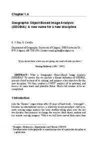
12 2.2.3 Quantum gates Quantum gates operate on qubits. These gates are conceptually similar to logic gates in the classical world. In the classical world the only non-trivial single bit gate is the Not gate which sends 0 to 1 and 1 to 0. However, there are infinitely many non-trivial quantum gates. An n−qubit quantum gate is represented by a 2n × 2n matrix. A necessary and sufficient condition for such a matrix to be a quantum gate is that it is unitary. The entanglement of two qubits, p and q, is accomplished by applying a Hadamard transformation to p followed by a Not applied to q controlled by p. The circuit in figure 2.2 on page 16 shows how to entangle two qubits that start with an initial state of |00i. See figure C.1 on page 145 for how this can be done in L-QPL. A list of some common gates, together with their usual quantum circuit representation is given in the next section in table 2.1 on page 17.

2.2.4 Measurement The other allowed operation on a qubit or group of qubits is measurement. When a qubit is measured it assumes only one of two possible values, either |0i or |1i. Given q = α |0i + β |1i

(2.4)

where |α|2 + |β|2 = 1, then measuring q will result in |0i with probability |α|2 and |1i with probability |β|2 . Once a qubit is measured, re-measuring will always produce the same value. In multi-qubit systems the order of measurement does not matter. If p and q are as in equation (2.1) on the preceding page, let us suppose measuring p gives |0i. The measure will result in that value with probability |α00 |2 + |α01 |2 , after which the system

13 collapses to the state: α00 |00i + α01 |01i

(2.5)

Measuring the second qubit, q, will give |0i with probability |α00 |2 or |1i with probability |α01 |2 . Conversely, if q was measured first and gave us |0i (with a probability of |α00 |2 + |α10 |2 ) and then p was measured, p will give us |0i with probability |α00 |2 or |1i with probability |α10 |2 . Thus, when measuring both p and q, the probability of getting |0i from both measures is |α00 |2 , regardless of which qubit is measured first. Considering states such as in equation (2.3), measuring either qubit would actually force the other qubit to the same value. This type of entanglement is used in many quantum algorithms such as quantum teleportation.

2.2.5 Mixed states The notion of mixed states refers to an outside observer’s knowledge of the state of a quantum system. Consider a 1 qubit system ν = α |0i + β |1i .

(2.6)

If ν is measured but the results of the measurement are not examined, the state of the system is either |0i or |1i and is no longer in a superposition. This type of state is written as: ν = |α|2 {|0i} + |β|2 {|1i}.

(2.7)

An external (to the state) observer knows that the state of ν is as expressed in equation (2.7). Since the results of the measurement were not examined, the exact state (0 or 1) is unknown. Instead, a probability is assigned as expressed in the equation.

14 Thus, if the qubit ν is measured and the results are not examined, ν can be treated as a probabilistic bit rather than a qubit.

2.2.6 Density matrix notation The state of any quantum system of qubits may be represented via a density matrix. In this notation, given a qubit ν, the coefficients of |0i and |1i form a column vector u. Then the density matrix corresponding to ν is uu∗ . If ν = α |0i + β |1i,    
α αα αβ ν= . α β = β βα ββ

(2.8)

When working with mixed states the density matrix of each component of the mixed state is added. For example, the mixed state shown in equation (2.7) on the preceding page would be represented by the density matrix    2    |α| 0 1 0 2 0 0 . = + |β| |α| 0 |β|2 0 1 0 0 2

(2.9)

Note that since the density matrix of mixed states is a linear combination of other density matrices, it is possible to have two different mixed states represented by the same density matrix. The advantage of this notation is that it becomes much more compact for mixed state systems. Additionally, scaling issues are handled by insisting the density matrix has a trace = 1. During a general quantum computation, as we shall see, the trace can actually fall below 1 indicating that the computation is not everywhere total. Gates and density matrices When considering a qubit q as a column vector and a unitary transform T as a matrix, the result of applying the transform T to q is the new vector T q. The density matrix of the original qubit is given by q q∗ , while the density matrix of the transformed qubit

15 is (T q)(T q)∗ , which equals T (qq∗ )T ∗ . Thus, when a qubit q is represented by a density matrix A, the formula for applying the transform T to q is T AT ∗ .

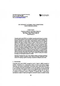
2.3 Quantum circuits 2.3.1 Contents of quantum circuits Currently a majority of quantum algorithms are defined and documented using quantum circuits. These are wire-type diagrams with a series of qubits input on the left of the diagram and output on the right. Various graphical elements are used to describe quantum gates, measurement, control and classical bits. Gates and qubits The simplest circuit is a single wire with no action: x

The next simplest circuit is one qubit and one gate. The qubit is represented by a single wire, while the gate is represented by a box with its name, G, inside it. This is shown in the circuit in figure 2.1. In general, the name of the wire which is input to the gate G may be different from the name of G’s output wire. Circuit diagrams may also contain constant components as input to gates as in the circuit in figure 2.3 on the following page. x

G

y

Figure 2.1: Simple single gate circuit Future diagrams will drop the wire labels except when they are important to the concept under discussion.

16 x

H

x′

y

•x

  y

′ ′

Figure 2.2: Entangling two qubits. |1i |1i

 

•

|0i |1i

Figure 2.3: Controlled-Not of |1i and |1i Controlled gates, where the gate action depends upon another qubit, are shown by attaching a wire between the wire of the control qubit and the controlled gate. The circuit in figure 2.2 shows two qubits, where a Hadamard is applied to the top qubit, followed by a controlled-Not applied to the second qubit. In circuits, the control qubit is on the vertical wire with the solid dot. This is then connected via a horizontal wire to the gate being controlled. A list of common gates, their circuits and corresponding matrices is given in table 2.1 on the following page. Measurement Measurement is used to transform the quantum data to classical data so that it may be then used in classical computing (e.g. for output). The act of measurement is placed at the last part of the quantum algorithm in many circuit diagrams and is sometimes just implicitly considered to be there. While there are multiple notations used for measurement in quantum circuit diagrams, this thesis will standardize on the D-box style of measurement as shown in figure 2.4. W

M2543

D-box

Figure 2.4: Measure notation in quantum circuits A measurement may have a double line leaving it, signifying a bit, or nothing,

17

Gate Not (X)

Z

Hadamard

Swap

Controlled-Not

Circuit

Matrix

 

  0 1 1 0

Z

  1 0 0 −1

H

√1 2

× ×

 1 0  0 0

0 0 1 0

0 1 0 0

 0 0  0 1

•

 1 0  0 0

0 1 0 0

0 0 0 1

 0 0  1 0

• •

 1 0  0  0  0  0  0 0

0 1 0 0 0 0 0 0

0 0 1 0 0 0 0 0

0 0 0 1 0 0 0 0

 

Toffoli

  1 1 1 −1

 

0 0 0 0 1 0 0 0

0 0 0 0 0 1 0 0

0 0 0 0 0 0 0 1

Table 2.1: Gates, circuit notation and matrices

 0 0  0  0  0  0  1 0

18 signifying a destructive measurement. Operations affecting multiple qubits at the same time are shown by extending the gate or measure box to encompass all desired wires. In the circuit in figure 2.5, the gate U applies to all of the first three qubits and the measurement applies to the first two qubits. ED

U

bitsBC

Figure 2.5: Examples of multi-qubit gates and measures

0-control and control by bits The examples above have only shown control based upon a qubit being |1i. Circuits also allow control on a qubit being |0i and upon classical values. The circuit in figure 2.6 with four qubits (r1 , r2 , p and q) illustrates all these forms of control. At g1 , a Hadamard is 1−controlled by r2 and is applied to each of r1 and p. This is followed in column g2 with the Not transform applied to r2 being 0−controlled by r1 . In the same column, a Z gate is 0−controlled by q and applied to p. p and q are then measured in column g3 and their corresponding classical values are used for control in g4 . In g4 , the UR gate is applied to both r1 and r2 , but only when the measure result of p is 0 and the measure result of q is 1. r1 r2 p

H

  

•

 

H

Z

q

  

g1

g2

UR   

ED

Mp,qBC g3

g4

•

Figure 2.6: Other forms of control for gates

19 Multi-qubit lines It is common to represent multiple qubits on one line. A gate applied to a multiqubit line must be a tensor product of gates of the correct dimensions. The circuit in figure 2.7 shows n qubits on one line with the Hadamard gate (tensored with itself n times) applied to all of them. That is followed by a unary gate UR tensored with I⊗(n−2) and tensored with itself again. This will have the effect of applying an UR gate to the first and last qubits on the line. n

/

UR ⊗ I⊗(n−2) ⊗ UR

H⊗n

Figure 2.7: n qubits on one line

Other common circuit symbols Two other symbols that are regularly used are the swap and controlled-Z, shown in the circuit in figure 2.8. Note that swap is equivalent to a series of three controlled-Not gates with the control qubit changing. This can also be seen directly by multiplying the matrices for the controlled-Not gates as shown in equation (2.10). × ×

≡ • Z

•

 

=

•

 

•

 

 

Figure 2.8: Swap and controlled-Z  1 0  0 0

0 0 1 0

0 1 0 0

  1 0   0 0 = 0 0 0 1

0 1 0 0

0 0 0 1

 0 1  0  0 1 0 0 0

0 0 0 1

0 0 1 0

 0 1  1  0 0 0 0 0

0 1 0 0

0 0 0 1

 0 0 . 1 0

(2.10)

20 2.3.2 Syntax of quantum circuits Quantum circuits were originally introduced by David Deutsch in [Deu89]. He extended the idea of standard classical based gate diagrams to encompass the quantum cases. In his paper, he introduced the concepts of quantum gates, sources of bits, sinks and universal gates. One interesting point of the original definition is that it does allow loops. Currently, the general practice is not to allow loops of qubits. The commonly used elements of a circuit are summarized in table 2.2 on the following page. A valid quantum circuit must follow certain restrictions. As physics requires qubits must not be duplicated, circuits must enforce this rule. Therefore, three restrictions in circuits are the no fan-out, no fan-in and no loops rules. These conditions are a way to express the linearity of quantum algorithms. Variables (wires) may not be duplicated, may not be destroyed without a specific operation and may not be amalgamated.

2.3.3 Examples of quantum circuits This section will present three quantum algorithms and the associated circuits. Each of the circuits presented may be found in [NC00]. First, quantum teleportation, an algorithm which sends a quantum bit across a distance via the exchange of two classical bits. This is followed by the Deutsch-Jozsa algorithm, which provides information about the global nature of a function with less work than a classical deterministic algorithm can. The third example includes circuits for the quantum Fourier transformation and its inverse. Quantum teleportation The standard presentation of this algorithm involves two participants Alice and Bob. In the diagrams, these will be labelled as A and B. Alice and Bob first initialize two qubits to |00i, then place them into what is known as an EPR (for Einstein, Podolsky

21

Desired element

Element in a quantum circuit diagram.

qubit

A single horizontal line.

Classical bit

A double horizontal line.

Single-qubit gates

A box with the gate name (G) inside it, one wire attached on its left and one wire attached on the right.

Multi-qubit gates

A box with the gate name (R) inside it, n wires on the left side and the same number of wires on the right.

Controlled qubit gates

A box with the gate name (H, W) inside, with a solid (1-control) or open (0control) dot on the control wire with a vertical wire between the dot and the second gate.

ControlledNot gates

A target ⊕, with a solid (1-control) or open (0-control) dot on the control wire with a vertical wire between the dot and the gate.

Measurement

A D-box shaped node with optional names or comments inside. One to n single wires are attached on the left (qubits coming in) and 0 to n classical bit wires on the left. Classical bits may be dropped as desired.

Classical control

Control bullets attached to horizontal classical wires, with vertical classical wires attached to the controlled gate.

Multiple qubits

Annotate the line with the number of qubits and use tensors on gates.

Example

G

R •

W

H

  

•

 

•

ED

H

r"%$#

q, rBC

• X

n

/

H⊗n

Table 2.2: Syntactic elements of quantum circuit diagrams

22 and Rosen) state. This is accomplished by first applying the Hadamard gate to Alice’s qubit, followed by a controlled-Not to the pair of qubits controlled by Alice’s qubit. Then, Bob travels somewhere distant from Alice, taking his qubit with him1 . At this point, Alice receives a qubit, ν, in an unknown state and has to pass ν on to Bob. She then uses ν as the control and applies a controlled-Not transform to this new pair. Alice then applies a Hadamard transform applied to ν. Alice now measures the two qubits and sends the resulting two bits of classical information to Bob. Bob then examines the two bits that he receives from Alice. If the bit resulting from measuring Alice’s original bit is 1, he applies the Not (also referred to as X) gate   0 1 (= ) to his qubit. If the measurement result of ν is one, he applies the Z gate 1 0   1 0 (= ). Bob’s qubit is now in the same state as the qubit Alice wanted to send. 0 −1 The circuit for this is shown in figure 2.9. |νi

•

A

 

H

•

M1 :=